Atmospheric predictability revisited

Abstract

Abstract

This article examines the potential to improve numerical weather prediction (NWP) by estimating upper and lower bounds on predictability by re-visiting the original study of Lorenz (1982) but applied to the most recent version of the European Centre for Medium Range Weather Forecasts (ECMWF) forecast system, for both the deterministic and ensemble prediction systems (EPS). These bounds are contrasted with an older version of the same NWP system to see how they have changed with improvements to the NWP system. The computations were performed for the earlier seasons of DJF 1985/1986 and JJA 1986 and the later seasons of DJF 2010/2011 and JJA 2011 using the 500-hPa geopotential height field. Results indicate that for this field, we may be approaching the limit of deterministic forecasting so that further improvements might only be obtained by improving the initial state. The results also show that predictability calculations with earlier versions of the model may overestimate potential forecast skill, which may be due to insufficient internal variability in the model and because recent versions of the model are more realistic in representing the true atmospheric evolution. The same methodology is applied to the EPS to calculate upper and lower bounds of predictability of the ensemble mean forecast in order to explore how ensemble forecasting could extend the limits of the deterministic forecast. The results show that there is a large potential to improve the ensemble predictions, but for the increased predictability of the ensemble mean, there will be a trade-off in information as the forecasts will become increasingly smoothed with time. From around the 10-d forecast time, the ensemble mean begins to converge towards climatology. Until this point, the ensemble mean is able to predict the main features of the large-scale flow accurately and with high consistency from one forecast cycle to the next. By the 15-d forecast time, the ensemble mean has lost information with the anomaly of the flow strongly smoothed out. In contrast, the control forecast is much less consistent from run to run, but provides more detailed (unsmoothed) but less useful information.

• numerical weather prediction
• predictability
• predictive skill
• ensemble prediction

1. Introduction

Forecast skill has improved dramatically in the recent decades (see for example, Simmons and Hollingsworth, 2002; Simmons, 2006). This is due to a number of factors, including increased computing power allowing higher resolution models to be run, improvements to the observing system and data assimilation and changes to the parameterisations used to represent sub-grid scale processes. The improvements to data assimilation systems alone have contributed significantly to the improvement in forecast skill by producing more accurate initial states (Simmons, 2006). Although forecast skill is continuously improving, there is an upper limit to this skill. This situation arises because of the chaotic nature of the atmosphere (Lorenz, 1963); two almost identical initial atmospheric states will always, given sufficient time, evolve into different future atmospheric states. Since it is not possible to determine the current state of the atmosphere exactly, small errors in the initial conditions will grow rapidly and result in a total loss of skill at longer lead times. Improving the initial state will clearly improve the forecasts, but improvements also depend on the forecast model itself. While numerical models are continuously improving, they are not perfect and provide only an approximation of the time evolution of the atmosphere. In particular, smaller scale features and processes are not explicitly resolved by the model. Their impacts on the larger scales are approximated using parameterisations, but the uncertainty of these smaller scales must also be taken into account. Lorenz (1969) showed that even if the larger resolved scales could be determined perfectly providing a perfect initial state, the uncertainties in the unresolved smaller scales would induce errors in the resolvable scales, often termed ‘backscatter’, which after some finite time would be more or less identical to a state with errors that already existed in the resolvable scales. Therefore, it is necessary to consider potential forecast skill and try to determine the upper limit to this skill; that is, the limit beyond which the forecast error cannot get any smaller by improving the forecast system.

To make the following discussion understandable to the general reader, we provide definitions of concepts that are used in this article. A deterministic system in mathematical physics is a system where the development of a future state is strictly determined by the governing equations and will always produce the same results from given initial and boundary conditions. We call such a forecast a deterministic forecast. An ensemble forecast consists of a given number of deterministic forecasts where each individual forecast starts from a slightly different initial state. Normally, the initial state is modified with selected perturbations that are also realistic possible initial states. Also, some aspects of the governing equations, such as the parameterisation of convection can also be perturbed, generally termed ‘stochastic physics’ (Buizza et al., 1999).

Following Lorenz (1969), we define deterministic predictability as the instant in time of an integration when the deviation of the integration from the true state of the atmosphere is equal in size to any state randomly selected from the true state of the atmosphere.

The limit of predictability or limit of deterministic forecasting will occur at a time when the predicted state deviates as much from the verifying state as a randomly selected, but dynamically and statistically possible state. An alternative definition is when it deviates more from the validating state than the average long-term mean (climate mean) deviates from the validating state. A predictability upper bound is the skill that is theoretically achievable with a perfect model for a given set of equations whereas forecast skill is what is actually achievable in a given numerical weather prediction (NWP) system that contains model errors, following Lorenz (1982) we will call this predictability lower bound. The potential forecast skill is the skill when the forecast error of such a system is nil.

Estimates of potential forecast skill can be obtained by comparing the integrations of a model started from slightly different initial states (Lorenz, 1965). An innovative approach to this was devised by Lorenz (1982), with the objective of quantifying upper and lower bounds of predictability. The lower bound was simply determined by calculating the current forecast skill of an operational system; that is, the root mean-square error (RMSE) between forecast data, of increasing lead times, and analysis data valid at the same time. The upper bound, or potential forecast skill, was determined by calculating the root mean-square (RMS) difference between consecutive pairs of forecasts, valid at the same time, but with lead times differing by some fixed time interval. For example, if this interval was 1 d, then the analysis for a given day would be compared with the 1-d forecast valid for the same day, then this 1-d forecast would be compared with the 2-d forecast valid for the same day and so on. Lorenz argued that even in the case of a perfect model that if two forecasts started from similar initial states (i.e., forecasts separated by 1 d) diverged at a similar rate to that at which two similar but distinct atmospheric states diverged, then the predictability measure described above could not be improved unless the 1-d forecast error was reduced (Lorenz, 1982).

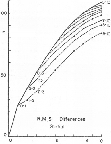
Figure 1 shows the predictability curves of the Lorenz (1982) study, which were calculated using a 100-d sequence of European Centre for Medium Range Weather Forecasts (ECMWF) operational forecasts of 500-hPa height fields from 1 December 1980 to 10 March 1981. The evolution of the predictability error (upper bound) was, as might be expected, smaller than the actual forecast error (lower bound). This method provides a convenient way to determine how errors of different sizes grow with increasing forecast lead time, giving a measure of potential forecast skill, and has been used in a number of more recent studies (e.g. Simmons et al., 1995; Simmons and Hollingsworth, 2002; Bengtsson and Hodges, 2005; Bengtsson et al., 2005).

Fig. 1 Taken from Lorenz (1982, Fig. 1). Upper and lower bound predictability curves calculated from the 500-hPa geopotential height field of the ECMWF forecast system for the 100-d period from 1 December 1980 to 10 March 1981 (for details see text).

The first objective of this article is to recalculate upper and lower bounds of atmospheric predictability using a recent version of the ECMWF forecast system to determine how these bounds have changed. It is then possible to consider how much potential remains to improve deterministic forecasting via changes to the model itself at least in terms of fields of this representative scale.

In the realisation of the inherent limitations of deterministic predictions, ensemble prediction methods have been developed (Leith, 1974; Toth and Kalnay, 1993, 1997; Buizza and Palmer, 1995; Molteni et al., 1996; Bengtsson et al., 2008) and are now routinely used in NWP by many operational weather centres (Buizza et al., 2007; Bowler et al., 2008; Wei et al., 2008; Charron et al., 2010). The ensemble approach involves the integration of multiple forecasts, each started from slightly different initial states to provide an estimate of the probability density function of forecast states (Leith, 1974). Additionally, some ensemble systems also introduce stochastic model physics where the model itself is perturbed to sample the model errors by introducing spatially and temporally correlated noise into the model physics schemes (Buizza, 1999). The control forecast is integrated from the analysis without any perturbations, initial state or stochastic, but at the same resolution as the ensemble members. The initial conditions for the other ensemble members are obtained by applying perturbations to the analysis, with the aim of sampling the probability density function of the errors in the initial state.

Ensemble prediction systems (EPS) have several advantages over deterministic forecasts. First, they provide a measure of the probability/uncertainty in a predicted weather event or synoptic condition. Individual ensemble members can also give warnings of extreme events earlier on in the forecast cycle than a single deterministic integration. An additional aim is that the average of the ensemble forecasts, the ensemble mean, will provide a forecast that is, although somewhat smooth, superior than the control forecast (Leith, 1974; Toth and Kalnay, 1993, 1997). However, as has been pointed out by Bengtsson et al. (2008), even if the ensemble mean is superior than any ensemble member beyond a certain time, it is dynamically inconsistent.

The second objective of this article is to assess the potential predictability of ensemble forecasting, using an approach that is analogous to Lorenz (1982), by calculating upper and lower bounds of predictability of the ensemble mean forecast.

Before continuing we note that, as in Lorenz (1982), our aim is to assess the predictability of medium-range synoptic-scale forecasting. The limits of predictability of higher resolution mesoscale forecasting will of course be very different, as will those of lower resolution seasonal- or climate-scale forecasting, and we do not consider these here.

This article is structured as follows: Section 2 provides a description of the ECMWF deterministic and ensemble systems we have used to calculate our predictability estimates. Section 3 presents the predictability estimates of a recent and older version of the ECMWF deterministic system and Section 4 presents the results for the ensemble system. This article ends with a discussion and conclusions in Section 5.

2. Forecast model data

We have used the ECMWF integrated forecast system (IFS) for both the deterministic and ensemble forecast predictability calculations. This choice was motivated by the desire to remain consistent with the Lorenz's (1982) study, which only used deterministic forecasts, but also because the ECMWF IFS has one of the highest levels of forecast skill of current operational weather centres (e.g. Park et al., 2008; Froude, 2010). Our predictability estimates may of course vary if a different forecast system were to be used.

In order to access how upper and lower bounds of predictability have changed, we have repeated Lorenz's calculations for the periods of DJF 1985/1986 and DJF 2010/2011. The earlier season was chosen because it is the earliest we have access to in the ECMWF data archive and the later was chosen because it was the most recent that we had available. The earlier season is approximately 5 yr later than the forecasts used in the Lorenz (1982) study. For robustness, we also performed the calculations for the JJA seasons of 1986 and 2011. During the earlier seasons of DJF 1985/1986 and JJA 1986, the ECMWF model was run at a spectral resolution of T106 (125 km) with 19 vertical levels. It was an Eulerian hybrid-coordinate model and used an optimum interpolation (OI) data assimilation scheme. During the more recent seasons of DJF 2010/2011 and JJA 2011 the model was run at the much higher resolution of T1279 (16 km) with 91 levels in the vertical. The model uses a semi-Lagrangian numerical scheme and a 4DVAR data assimilation (e.g. Rabier et al., 2000) system. Both versions of the ECMWF model are integrated out to 10 d.

We have also performed predictability calculations analogous to Lorenz (1982), for the ECMWF ensemble mean and control forecasts for the season of DJF 2010/2011. The EPS uses the same model as the high-resolution deterministic model, but it is run at the lower resolution of T639 with 62 vertical levels for the first 10 days of the forecast. It is then integrated for a further 5 days, providing forecasts out to 15 d, but at the reduced resolution of T319 (still with 62 vertical levels). The ECMWF EPS consists of 50 perturbed ensemble members and a control forecast. Initial condition perturbations are constructed using initial-time singular vectors and an ensemble of data assimilations [(EDA), Buizza et al., 2010]. In addition to the initial condition perturbations, random perturbations are applied to the parameterised physical processes (stochastic physics, Buizza et al., 1999) to represent the model uncertainty.

To be consistent with Lorenz (1982), we use the 500-hPa height fields in all our calculations to assess predictability. This field is also a very good predictor of general weather patterns and is therefore a suitable field to analyse, although we recognise that the results may be different if another parameter were used such as winds or precipitation. We have analysed data generated using models at different resolutions, but have performed all our calculations at a common resolution of T106 to maintain consistency. To assess whether this has any impact on the results we also performed the calculations at a resolution of T42. There was no difference in the results and we therefore feel confident that performing our analysis at T106 will not affect our results. All analysis was performed separately for the Northern Hemisphere (20°, 90°, NH) and Southern Hemisphere (−90°,−20°, SH).

3. Deterministic forecasts

Upper and lower bounds of atmospheric predictability as in Lorenz (1982) were calculated for the DJF seasons and are shown in Fig. 2a and b for the NH and SH, respectively. The thick black curves in the figure show the lower bound, which is simply the averaged forecast skill calculated as the RMS between forecasts and analyses for the DJF 1985/1986 season. This is a lower bound since we know that forecasts can achieve at least this level of predictive skill. The thin black curves were calculated, again as per Lorenz (1982), as the RMS difference between consecutive pairs of forecasts, valid at the same time, but with lead times differing by some fixed interval. The curve with the smallest errors is calculated using a fixed interval of 1 d; that is, the 1-d forecasts are compared with the analyses valid at the same time, then the 2-d forecasts are compared with the 1-d forecasts valid at the same time, the 3-d with the 2-d forecasts and so on. As described by Lorenz (1982), this gives a measure of how much potential there is to improve the skill of the forecasts via changes to the model. The thin black curves with the second smallest errors are calculated with a 2-d displacement and therefore show how much potential there is to improve the forecast without reducing the 2-d forecast error. The next lower black curves are calculated with a 3-d fixed interval and so on. The red curves of the figure are the same as the black but for the later period of DJF 2010–2011.

Fig. 2 Upper and lower bound predictability curves calculated from the 500-hPa geopotential height field of the ECMWF deterministic forecasts, in the same way as Lorenz (1982), for the DJF 1985/1986 (black curves) and DJF 2010/2011 (red curves) seasons in (a) the NH and (b) the SH and for the JJA 1985 (black curves) and JJA 2011 (red curves) seasons in (c) the NH and (d) the SH.

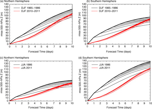
As would be expected, the lower bound of predictability has been reduced considerably in the later DJF season, indicating an improvement in forecast skill of approximately 2 d (i.e., the 10-d forecast of the later DJF season has the same level of skill as the 8-d forecast of the earlier one). This is partly due to model improvements, but also to a significant reduction of the initial error due to better observations and to more advanced data assimilation. It is also apparent that the predictability curves are much closer together in the later DJF season than the earlier one. This would again be expected since as forecast models are improved they will provide a more and more realistic representation of the true atmospheric evolution. It is interesting just how close the predictability curves for the more recent season have become, indicating that we may be approaching a limit of predictability of the deterministic forecast, at least for 500-hPa height field, and further improvements might require further reduction of the initial error. This will in turn require an improvement of the fully integrated forecasting system.

Another interesting observation from Fig. 2a and b is that the predictability curves for the later DJF season have a steeper gradient from about day 3 of the forecast compared to the earlier DJF season. Later in the forecast integration, from about day 6, they intersect the predictability curves of the earlier season and have larger errors. This suggests that estimates of potential predictability calculated from earlier versions of the forecast model, such as those of Lorenz (1982) and our calculations for DJF 1985/1986, are a little on the optimistic side. Indeed, Lorenz (1982) pointed out that it is possible that as the model is continually made more realistic, the estimate of the doubling times, which can be calculated from the predictability curves will decrease, bringing the top and bottom curves closer together. It seems that this is the case to some extent and that the internal variability of earlier versions of the model was insufficient (see Figs. 2 and 3).

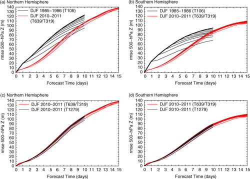
Fig. 3 Upper and lower bound predictability curves calculated from the 500-hPa geopotential height field of the ECMWF deterministic forecast for DJF 1985/1986 (black curves) and the ECMWF control forecast for DJF 2010/2011 (red curves) in (a) the NH and (b) the SH. The curves are also shown for the ECMWF deterministic forecast (black) and control forecast (red) for DJF 2010/2011 in (c) the NH and (d) the SH. All predictability estimates are calculated in the same way as Lorenz (1982).

For completeness of our results, we also calculated the predictability estimates for the JJA seasons of 1986 and 2011. The results are shown in Fig. 2c and d for the NH and SH, respectively. As would be expected the errors are larger for the SH winter and smaller for the NH summer. Furthermore, the estimates of potential predictability calculated from earlier versions of the ECMWF model are slightly too high because of a more rapid error growth of the later model. While these results appear to suggest that we have nearly approached a limit of deterministic forecasting and that no further improvements can be made unless the initial error is further reduced, some caution should be exercised. At longer lead times, the error associated with the chaotic nature of the atmosphere may dominate those associated with model error making it difficult to determine improvements associated with improving the model. Focussing more on the short range of the forecast, Magnusson and Källén (2013) found that the impact of improving the model was discernible from the chaotic error and that it is linked to the initial state, so that initial state improvements are also a consequence of the model improvement.

The ECMWF deterministic forecasts are integrated out to 10 d and we can therefore only show the predictability curves of Fig. 2 out to this point. However, it is interesting to consider what happens to these curves beyond this point. To do this, we computed the predictability curves for the control forecast from the ECMWF EPS. This is a lower resolution version of the deterministic forecast but is integrated out to 15 d. In Fig. 3a and b, the predictability curves for the control forecast are shown in red out to 15 d for the DJF 2010/2011 season in the NH and SH, respectively. The predictability curves from the deterministic forecast of the earlier DJF 1985/1986 season are also shown in black out to 10 d for comparison. By the 15-d forecast time, the curves have begun to level off (particularly in the SH) at a value slightly higher than the lower bound estimate of predictability of the earlier season. It seems therefore that the limit of deterministic predictability of about 2 weeks of the large-scale 500-hPa height field proposed by Lorenz (1982) is also supported by this study. For completeness, we have also shown in Fig. 3c and d the control forecast predictability curves and the deterministic predictability curves, both for the DJF 2010/2011 season, in order to assess the impact of doubling the resolution of the forecast. The curves are practically identical showing that increasing the resolution any further will probably have limited impact on the prediction of the 500-hPa height field.

4. Ensemble forecasts

As discussed in Section 1, ensemble weather prediction was developed, in recognition of the inherent limits of deterministic prediction, to provide an estimate of the forecast uncertainty. In this section, we consider how ensemble forecasting can extend deterministic predictability limits.

4.1. Ensemble mean predictability statistics

Figure 4 shows the predictability curves calculated for the ECMWF ensemble mean forecasts. Figure 4a and c shows the results for the DJF 2010/2011 season in the NH and SH, respectively. The top thicker curves, as in the earlier figures, correspond to the forecast skill (lower bound) of the ensemble mean forecast and the thinner curves are the predictability curves calculated with different initial differences. Since the ensemble forecasts are produced every 12 h, the bottom curves with the smallest errors were obtained using a 12-h fixed interval; that is, by comparing the 0.5-d forecasts with the analyses valid at the same time, the 1-d forecasts with the 0.5-d forecasts valid at the same time, the 1.5-d forecasts with the 1-d forecasts and so on. The next curve up, with the second smallest error, will have a 1-d fixed interval, the next a 1.5-d interval and so on. This was not possible in the earlier figures as the forecast model was only integrated once a day during the earlier DJF 1985/1986 season. Figure 4b and d shows the predictability curves for the control forecast in the NH and SH, respectively. Since the control forecast is run at the same resolution as the perturbed ensemble members, it is the deterministic equivalent of the ensemble forecast curves.

Fig. 4 Upper and lower bound predictability curves calculated from the 500-hPa geopotential height field of the ECMWF ensemble mean forecasts, analogous to Lorenz (1982) but every 12 h, for the DJF 2010/2011 season in (a) the NH and (b) the SH. The predictability curves are also shown for the control forecast in (b) the NH and (d) the SH.

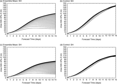
It is no surprise that the actual forecast error (lower predictability) bound of the ensemble mean forecast is smaller than that of the control forecast in both hemispheres, since this is one of the motivations for running an EPS. By the 10-d forecast time, the ensemble mean error is >20% smaller than the control in both hemispheres. What is more striking, however, is the difference in the potential predictability curves. The error growth of these curves is dramatically smaller than for the deterministic case, beginning to level off at around 7 d and even reducing from around 10 d. It can be considered that a useful forecast system should have a monotonously increasing forecast error with a forecast lead time until an asymptotic limit is reached. Hence, a possible interpretation of the decreasing error is that once the curves start to decrease then the ensemble mean is starting to loose predictive skill.

Current EPS are set up in such a way that all members are not equally likely, as one of the members (control) constitutes the most likely case and all other cases are perturbed around this case with the objective of selecting those perturbations that are expected to have the fastest growth.

Let us assume that we undertake an ensemble experiment with a perfect model and an unlimited ensemble size. After a certain time of integration, such a forecasting system will produce a result with the ensemble mean identical to the climate. Assuming that we already know the climate, such a forecast will have no predictive skill. It therefore follows that the predictive skill of the ensemble mean forecast will be extended in time, but at the same time it will also become a smoother field with less variance than an individual member of the ensemble. This is likely to be an evolving process as for the short-range predictions the ensemble members are very similar so the mean will initially have almost as much variance as individual members and probably a similar error growth. However, the variance of the ensemble mean will gradually diminish as different members will evolve differently and some (unpredictable) variance in individual members will be averaged out. As a consequence, the ensemble mean will become more smoothed out. In order to understand and illustrate this further, we will now consider two case studies of the ensemble mean forecast.

4.2. Case studies example 1: 00 UTC 8 December 2010

The first forecast example we consider is for 00 UTC 8 December 2010, when Europe experienced exceptionally cold weather conditions. The cold spell began over Scandinavia during November and towards the end of the month moved southwest over Belgium, the Netherlands and the United Kingdom. Our first forecast example occurs towards the end of a 2-week spell of severe winter weather over the United Kingdom, between 25 November and 9 December. The United Kingdom experienced cold north-easterly winds from northern Europe and Siberia, together with snow.

Figure 5 shows the analysed 500-hPa height field for this time together with the 9-, 9.5- and 10-d control and ensemble mean forecasts valid at the same time. The RMS between the 9- and 9.5-d forecasts will have been used to calculate the values of the bottom curves (upper bound predictability estimate) in Fig. 4 at the 9-d forecast time. Similarly, the RMS between the 9.5- and 10-d forecasts has been used to calculate the values at the 9.5-d forecast time. For the second curve from the bottom, the RMS of the 9- and 10-d forecasts has been included at the 9-d forecast time. By studying this forecast example, we may be able to gain further insights and understanding of the predictability curves of Fig. 4.

Fig. 5 ECMWF analysis and 9-, 9.5- and 10-d control and ensemble mean forecasts of 500-hPa geopotential height valid at 00 UTC 8 December 2010 over the NH.

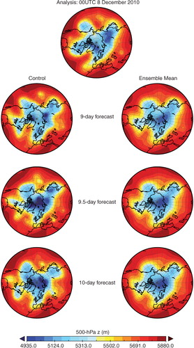
It is clear from Fig. 5 that the ensemble mean forecasts are much smoother than the control forecasts. The control forecasts have more detail, but there is less consistency between the different forecast cycles. Indeed, the consistency of the ensemble mean forecast is a property that has been noted before (Zsoter et al., 2009). On closer inspection of the figure, we see that while the ensemble mean forecasts are smoother than the control, the main features (a wave number 5 pattern) of the analysis are rather well predicted. The control forecast on the other hand does not predict these features with such consistency.

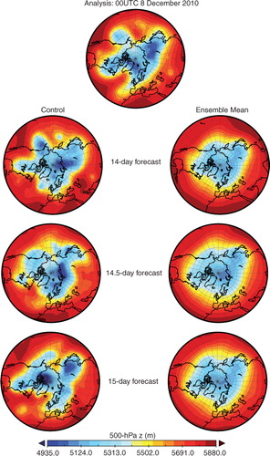
In order to explore what happens at longer lead times, Fig. 6 shows the 14-, 14.5- and 15-d control and ensemble mean forecasts for the same valid time. Here it is apparent that the ensemble mean has lost information with the anomaly of the flow strongly smoothed out. The consistency between forecast cycles is maintained, which will lead to the small RMSE values of the bottom predictability curve of Fig. 4a. In contrast, the inconsistency of the control forecast between cycles is apparent and will lead to the larger RMSE values of the bottom predictability curve of Fig. 4b. By this forecast lead time, the control forecast clearly provides more detailed forecast information than the ensemble mean, but this is not necessarily accurate information and false signals will be an issue. In summary, the ensemble mean forecast has become significantly smooth by this time, but the information it provides is more robust than that of the control.

Fig. 6 The same as Fig. 5 but for the 14-, 14.5- and 15-d forecasts.

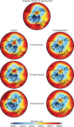
4.3. Case study example 2: 00 UTC 15 January 2011

The second forecast example we consider is the later date of 00 UTC 15 January 2011 when the earlier cold conditions had subsided and milder weather conditions were experienced in Europe. Figure 7 shows the analysed 500-hPa height field for this time together with the 9-, 9.5- and 10-d control and ensemble mean forecasts valid at the same time. There is an interesting blocking feature far north over Siberia and into the Arctic Ocean, which is well predicted by both the control and ensemble mean forecasts. As in the previous example from December, the ensemble mean forecasts are more consistent between forecast runs, but are smoother and have less detail than the control forecasts. For this particular case, both the control and ensemble mean forecasts are skilful in predicting the main features of the large-scale flow.

Fig. 7 The same as Fig. 5 but for 00 UTC 15 January 2011.

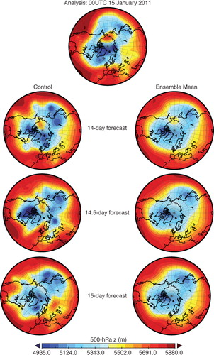
Figure 8 shows the 14-, 14.5- and 15-d control and ensemble mean forecasts for this date. The ensemble mean forecasts are more smoothed out than the earlier forecast times, but the main features of the flow are still indicated. The blocking high is weaker in all the forecasts, but is still present (although is not as apparent in the 14.5 and 15-d forecasts due to the particular colour scale that we have used in the plots). Again the control forecasts have much more detail, but the downside is the false information being giving. This is more apparent here than in the previous December case (Fig. 6). For example, the 14.5-d forecast has an area of high 500-hPa height values that extends right up over Scandinavia, which is not present in the analysed field. The control forecasts are much less consistent between forecast cycles than the ensemble mean, again resulting in the larger RMSE values of the bottom predictability curve (Fig. 4b) compared with those of the ensemble mean (Fig. 4a).

Fig. 8 The same as Fig. 6 but for 00 UTC 15 January 2011.

5. Discussion and conclusion

This study has recalculated upper and lower bounds of atmospheric predictability analogous to Lorenz (1982) using both recent and older versions of the ECMWF forecast system. We note that we are only considering medium-range prediction of the large-scale atmospheric flow and have neither considered smaller meso-scale predictions on shorter timescales nor long-term predictions of climate, which will of course have different limits of predictability. The ECMWF system is one of the highest performing operational systems (Park et al., 2008; Froude, 2010), so systems with lower levels of forecast skill will be likely to have larger differences between upper and lower estimates of predictability. However, it appears that the forecast skill of the ECMWF system is now close to the maximum skill we can obtain for a deterministic forecast without further reducing the error in the initial state. Irrespective, that we are dealing with a different model than Lorenz (1982) the results confirm the findings by Lorenz that the limit of deterministic predictability of the large-scale atmospheric flow is about 2 weeks. This will likely be different at smaller spatial scales where errors saturate more quickly as shown by Lorenz (1969).

Our predictability calculations with the recent version of the ECMWF model suggest that those with earlier versions of the model; that is Lorenz (1982) and our own calculations with earlier versions of the model overestimate the upper bound of predictability. That is, they are a little optimistic in how much potential there is to improve predictions via changes to the model. We believe that this is due to insufficient internal variability in earlier versions of the model and that as the model has improved, it has become more realistic in its representation of the evolution of the true atmospheric flow.

In this article, we also performed the same predictability calculations with the ensemble mean of the ECMWF EPS to determine the potential of ensemble forecasting. The results we obtained with the ensemble mean were quite striking, indicating that the ensemble system has great potential in supporting the deterministic system. However, as the forecast progresses, the ensemble mean is becoming more smoothed out and provides less information. From around the 10-d lead time, the RMSE of the predictability calculations actually begins to decrease as it is beginning to converge towards climatology. Therefore, with increasing forecast time the added value of the ensemble mean is traded for a reduction in predictive information (above climatology).

In order to understand this result a little more, we considered two forecast examples and compared the ensemble mean forecasts against the control. While the control provided more detail than the ensemble mean, it was much less consistent between forecast cycles than the ensemble mean and consequently has much less predictability. At around the 9 to 10-d forecast time (just before the predictability curves begin to converge to climatology), the ensemble mean does very well at predicting the main features (wave numbers 1–5) of the atmospheric flow and is very consistent from run to run. By the 14 to 15-d forecast, much of the predictive information has been smoothed out in the ensemble mean forecast. The ensemble mean is still very consistent, but the anomaly of the flow is now strongly smoothed out. On the other hand, the control forecast is inconsistent between runs but provides more predictive information. However, the limits of deterministic predictability mean that at longer lead times this predictive information is becoming less and less accurate. At long lead times, the control forecast will also give false information and signals.

Forecast systems, such as that of ECMWF, are continuously being developed and improved. There are many ways in which this can be achieved such as increased resolution, improved model parameterisations, better observations and assimilation of those observations and the use of ensemble methods. The results of this article indicate that for deterministic forecasting (at least of the large-scale flow) it is important that improvements of the forecasting system be undertaken in such a way that it reflects in a reduced initial error. Ensemble methods are also an area with huge potential as they potentially indicate areas where the predictive skill is more robust.

6. Acknowledgements

The authors thank ECMWF for providing the deterministic and ensemble forecast data used in this study. They also thank the two reviewers and Prof. Erland Källén in particular, for their constructive comments.

References

- Bengtsson L , Hodges K. I . A note on atmospheric predictability. Tellus. 2005; 58A: 154–157.
- Bengtsson L , Hodges K. I , Froude L. S. R . Global observations and forecast skill. Tellus. 2005; 57A: 515–527.
- Bengtsson L. K , Magnusson L , Källén E . Independent estimations of the asymptotic variability in an ensemble forecasting system. Mon. Wea. Rev. 2008; 136: 4105–4112.
- Bowler N. E , Arribas A , Mylne K. R , Robertson K. B , Beare S. E . The MOGREPS short-range ensemble prediction system. Q. J. Roy. Meteorol. Soc. 2008; 134: 703–722.
- Buizza R , Palmer T. N . The singular-vector structure of the atmospheric global circulation. J. Atmos. Sci. 1995; 52: 1434–1456.
- Buizza R , Bidlot J.-R , Wedi N , Fuentes M , Hamrud M , co-authors . The new ECMWF VAREPS (variable resolution ensemble prediction system). Q. J. Roy. Meteorol. Soc. 2007; 133: 681–695.
- Buizza R , Leutbecher M , Isaksen L , Haseler J . The use of EDA perturbations in the EPS. ECMWF Newsletter, No. 2010; 123: 22–28.
- Buizza R , Miller M , Palmer T. N . Stochastic representation of model uncertainties in the ECMWF ensemble prediction system. Q. J. Roy. Meteorol. Soc. 1999; 125: 2887–2908.
- Charron M , Pellerin G , Spacek L , Houtekamer P. L , Gagnon N , co-authors . Towards random sampling of model error in the Canadian ensemble prediction system. Mon. Wea. Rev. 2010; 138: 1877–1901.
- Froude L. S. R . TIGGE: comparison of the prediction of Northern Hemisphere extratropical cyclones by different ensemble prediction systems. Wea. Forecasting. 2010; 25: 819–836.
- Leith C. E . Theoretical skill of Monte Carlo forecasts. Mon. Wea. Rev. 1974; 102: 409–418.
- Lorenz E. N . Deterministic Nonperiodic Flow. J. Atmos. Sci. 1963; 20: 130–141.
- Lorenz E. N . A study of the predictability of a 28-variable model. Tellus. 1965; 17: 321–333.
- Lorenz E. N . The predictability of a flow which possesses many scales of motion. Tellus. 1969; 21: 2890–2307.
- Lorenz E. N . Atmospheric predictability experiments with a large numerical model. Tellus. 1982; 34: 505–513.
- Magnusson L , Källén E . Factors influencing skill improvements in the ECMWF forecasting system. Mon. Wea. Rev. 2013. in press, DOI: 10.1175/MWR-D-12-00318.1.
- Molteni F , Buizza R , Palmer T. N , Petroliagis T . The ECMWF ensemble prediction system: methodology and validation. Q. J. Roy. Meteorol. Soc. 1996; 122: 73–119.
- Park Y.-Y , Buizza R , Leutbecher M . TIGGE: preliminary results on comparing and combining ensembles. Q. J. Roy. Meteorol. Soc. 2008; 134: 2029–2050.
- Rabier F , Järvinnen H , Klinker E , Mahfouf J.-F , Simmons A . The ECMWF operational implementation of four-dimensional variational assimilation. I: experimental results with simplified physics. Q. J. Roy. Meteorol. Soc. 2000; 126: 1143–1170.
- Simmons A. J , Palmer T , Hagedorn R . Observations, assimilation and the improvement of global weather prediction – some results from operational forecasting and ERA-40. Predictability of Weather and Climate. 2006; Cambridge University Press, Cambridge, UK.. 428–458.
- Simmons A. J , Hollingsworth A . Some aspects of the improvement in skill of numerical weather prediction. Q. J. Roy. Meteorol. Soc. 2002; 128: 647–677.
- Simmons A. J , Mureau R , Petroliagis T . Error growth and estimates of predictability from the ECMWF forecasting system. Q. J. Roy. Meteorol. Soc. 1995; 121: 1739–1771.
- Toth Z , Kalnay E . Ensemble forecasting at NMC: the generation of perturbations. Bull. Am. Meteorol. Soc. 1993; 74: 2317–2330.
- Toth Z , Kalnay E . Ensemble forecasting at NCEP and the breeding method. Mon. Wea. Rev. 1997; 125: 3297–3319.
- Wei M , Toth Z , Wobus R , Zhu Y . Initial perturbations based on the ensemble transform (ET) technique in the NCEP global operational forecast system. Tellus. 2008; 60A: 62–79.
- Zsoter E , Buizza R , Richardson D . ‘Jumpiness’ of the ECMWF and UK Met Office EPS control and ensemble-mean forecasts. Mon. Wea. Rev. 2009; 137: 3823–3836.