Causes and consequences of mid–21st-century rapid ice loss events simulated by the Rossby centre regional atmosphere-ocean model

Abstract

Recent observations and modelling studies suggest that the Arctic climate is undergoing important transition. One manifestation of this change is seen in the rapid sea-ice cover decrease as experienced in 2007 and 2012. Although most numerical climate models cannot adequately reproduce the recent changes, some models produce similar Rapid Ice Loss Events (RILEs) during the mid–21st-century. This study presents an analysis of four specific RILEs clustered around 2040 in three transient climate projections performed with the coupled Rossby Centre regional Atmosphere-Ocean model (RCAO). The analysis shows that long-term thinning causes increased vulnerability of the Arctic Ocean sea-ice cover. In the Atlantic sector, pre-conditioning (thinning of sea ice) combined with anomalous atmospheric and oceanic heat transport causes large ice loss, while in the Pacific sector of the Arctic Ocean sea-ice albedo feedback appears important, particularly along the retreating sea-ice margin. Although maximum sea-ice loss occurs in the autumn, response in surface air temperature occurs in early winter, caused by strong increase in ocean-atmosphere surface energy fluxes, mainly the turbulent fluxes. Synchronicity of the events around 2040 in the projections is caused by a strong large-scale atmospheric circulation anomaly at the Atlantic lateral boundary of the regional model. The limited impact on land is caused by vertical propagation of the surface heat anomaly rather than horizontal, caused by the absence of low-level temperature inversion over the ocean.

• coupled regional climate model
• rapid ice loss events
• Arctic
• climate scenarios
• sea-ice

1. Introduction

Climate change, induced by increased anthropogenic emissions of greenhouse gases (GHG), is one of the greatest environmental issues today. These changes are being experienced particularly intensely in the Arctic, where the temperatures have risen at almost twice the rate of the rest of the world in the past few decades (ACIA, 2005). The climate change projections realised with coupled general circulation models for the 21st century for the region suggest further warming. It should be noted though that the uncertainties in the projections for the Arctic are larger compared to those for lower latitudes, as shown by the large spread amongst models that participated in the third World Climate Research Program's (WRCP) Coupled Model Intercomparison Project (CMIP3). Understanding the changes in the Arctic climate is crucial not only for regional environmental and social issues, but also for global climate due to interconnections between the Arctic and global climates.

The Arctic sea-ice cover and its thickness, due to the relation to atmospheric and oceanic temperatures, is a sensitive indicator of climate change in the region. According to Stroeve et al. (2007), the September Arctic sea-ice extent has decreased during the 1979–2006 period at rates of 9.1% per decade. The recent years, however, showed accelerated summer sea-ice loss with 2007, 2011 and 2012 showing historical minimum values in the satellite observation era (Comiso et al., 2008; Fetterer et al., 2002). Nghiem et al. (2007), using observations and a drift-age model, suggested large acceleration in the rate of decrease of thick perennial (multi-year) ice reaching unprecedented values of 23% between March 2005 and March 2007. The transition from thicker perennial ice towards thinner first-year ice over the 2006–2007 period made the ice more vulnerable, leading to the summer historical minimum values of 2007 (Nghiem et al., 2007).

In addition, a number of other mechanisms also contributed to this rapid-observed decrease in sea-ice extent. The large-scale atmospheric circulation played an important role; for example, Deser and Teng (2008) and Wang et al. (2009) showed that trends in sea-ice cover over the marginal ice zones can be linked to the Northern Annular Mode (NAM) through the surface wind anomalies. This circulation anomaly strengthened the transpolar-drift, with anomalous meridional wind blowing from the western to the eastern Arctic, thus enhancing export of sea ice through Fram Strait. Nghiem et al. (2007) also showed observational evidence of increased inclusion of perennial (thick multi-year) ice in the transpolar drift, leading to massive ice volume exports through Fram Strait during the 2006–2007 period. However, the analysis by Deser and Teng (2008) concluded that the circulation anomalies could not explain the overall summer and winter trends in the sea-ice cover.

Kay et al. (2008) studied cloud cover and its potential links to the rapid decrease in sea ice during the 2006–2007 period. They reported a 16% decrease in summertime cloudiness over the Western Arctic from satellite and ground-based data in 2006 and 2007, which leads to an increase in downwelling short-wave radiation of 32W/m², while little changes in downwelling long-wave radiation (−4W m⁻²) were observed. The analysis of the changes in clouds and radiation over the summer melt season showed the potential to increase surface melting by 0.3m or 2.4K warming of the sea surface temperature (SST), energy potentially used for bottom melting of the ice. Although this anomaly of reduced cloudiness is not unprecedented in records, Kay et al. (2008) suggest that the presence of thinner sea-ice over the region made the system more vulnerable. This suggests that, in the future, anomalies in cloud cover and radiative fluxes might play an increasingly important role in regulating summer sea-ice extent. Observations of the ice mass balance over the Beaufort Sea confirmed a large increase in the bottom melting of the ice, mainly in 2007, caused by increased upper ocean temperature due to increased short-wave absorption, triggering an ice-albedo feedback and accelerated the sea-ice melt (Perovich et al., 2008).

Investigation of the Arctic climate using coupled general circulation models showed that none of the models contributing to CMIP3 were able to reproduce the observed acceleration of the Arctic sea-ice loss. Stroeve et al. (2007) clearly showed that CMIP3 coupled general circulation models underestimate the sensitivity of the Arctic sea ice to external forcing caused by the increase in GHG concentration. Analysis performed with the Community Climate System Model version 3 (CCSM3; Collins et al., 2006) showed rapid decreasing trends, suggesting nearly ice-free conditions by approximately 2050 (Holland et al., 2006, hereafter H06), while other models in the CMIP3 ensemble do not reach such state by 2100 (Stroeve et al., 2007). These results highlight the existing uncertainties in the simulation of the Arctic climate and the need for further investigation.

The modelled transition from perennial sea-ice cover to nearly ice-free summer often shows abrupt sea-ice reduction periods with trends similar in magnitude to those observed during the recent 2006–2012 period. These Rapid Ice Loss Events (RILEs) are characterised by abrupt summer sea-ice extent reduction over short time periods (5–10 yr). Using the CCSM3, Holland et al. (2006), in an assessment of the relative roles of natural and forced changes in sea-ice loss, identified multiple mechanisms responsible for such abrupt reduction in sea-ice cover. The long-term thinning over multiple decades occurring before the RILEs increased the vulnerability of the sea-ice cover, while ‘pulse-like’ ocean heat transport anomalies were found to be the triggering mechanism for rapid sea-ice loss. Once the ice loss has been triggered, a positive sea-ice albedo feedback occurs in CCSM3, further accelerating the sea-ice melt leading to extensive Arctic sea-ice loss. Holland et al. (2008, hereafter H08) suggested that the increased vulnerability of the sea ice caused by anthropogenic forcing results in an increase in the intrinsic variability of the sea-ice cover.

One of the important concerns related to the RILEs is to understand the consequences on the Arctic climate system. Under conditions of reduced sea-ice cover, the atmosphere comes in contact with the warm ocean waters leading to low-level atmospheric warming through increased turbulent fluxes at the surface. Surface winds can later advect this warm air towards surrounding land masses, further accelerating the general warming due to climate change over the adjacent permafrost underlain regions. This accelerated warming during RILEs can accelerate permafrost degradation (Lawrence et al., 2008) already observed in some parts of the Arctic, thus impacting soil thermal and moisture regimes, which can have an influence on the pan-Arctic biome. Another potential hazard is the release of soil carbon sequestered in the frozen ground, likely in methane form, to the atmosphere causing a positive feedback leading to further increase in temperature in future climate.

In a previous study, Döscher and Koenigk (2013; hereafter DK) studied 30 sea-ice reduction events in an ensemble of six regional Arctic climate scenarios from the Rossby Centre regional Atmosphere-Ocean model (RCAO) (Döscher et al., 2002, 2009). DK studied sea-ice reduction events throughout the 1980–2080 period in order to identify physical processes leading to these reductions. In DK, sea-ice reduction events are defined as summer sea-ice cover reduction of 1200000km² over a single or multiple successive years. This criterion is less constraining compared to that of H08 and the present study, and allowed them to perform statistical analysis over 30 less extreme sea-ice reduction events. DK suggested that sudden ice loss mechanisms were strongly related to changes in the large-scale atmospheric circulation and also influenced by sea-ice thinning as a pre-conditioning. Clustering of RILEs during the 2030–2035 period amongst the regional scenarios was indicative of a strong control of large-scale atmospheric forcing from the lateral boundary condition from ECHAM5/MPI-OM common scenario (hereafter ECHAM). Relating RILEs to atmospheric circulation anomalies, DK generally concluded that RILEs in RCAO could result from changes to the large-scale atmospheric circulation with very limited impact of seasonal radiative forcing on average.

This study aims to provide a more comprehensive understanding of the physical mechanisms responsible for four specific extreme RILEs simulated by RCAO clustered around 2040 with additional analysis of aspects not addressed in the previous study by DK. Detailed analysis of the surface energy fluxes and surface temperature is presented for the pre-RILE period, during the RILE and post-RILE period. Strong relations between RILEs and the changes in the atmospheric and oceanic circulation are established to demonstrate the important role played by the large-scale flows in the synchronicity of the extreme RILEs. In addition, we investigate the impacts of RILEs on the sea-ice variability and the atmospheric structure along with the regional response of temperature over the nearby coastal areas.

The outline of this article is as follows. Section 2 provides a brief description of the RCAO formulation and the model integrations. RCAO present-day climatology for the climate projections and comparison with the driving model ECHAM is presented in Section 3, while RILE analysis is presented in Section 4, followed by discussion and conclusions in Section 5.

2. Model description and experimental design

2.1. Model description

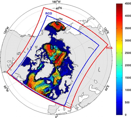
The Arctic regional climate projections considered in this study are performed by the RCAO (Döscher et al., 2002 and 2009) which consists of RCA for the atmosphere (Jones et al., 2004a, b; Kjellström et al., 2005) and RCO for the ocean (Meier et al., 2003). The model domain is centred over the Arctic and extends from approximately 50°N in the North Atlantic to the Aleutian Islands in the North Pacific (Fig. 1). The RCA domain was chosen in a way to avoid large orographic features near the lateral boundaries, while covering large enough areas to get realistic wind forcing over the Bering Sea. Both RCA and RCO are integrated at 0.5° horizontal resolution, on a rotated latitude–longitude grid for RCA and a spherical grid for RCO.

Fig. 1 RCAO arctic domain and bathymetry (m).

The RCO ocean model is based on the parallelised 3-D primitive equation model in geopotential coordinates with a free surface (Webb et al., 1997). Detailed description of the model formulation and evaluation can be found in Meier et al. (2003) and Döscher et al. (2009). RCO has 59 unevenly distributed vertical levels with the bottom topography interpolated from ETOPO5 data set (1988). Vertical resolution is 3m at the surface gradually decreasing to 200m at 5000m. The Aleutian Islands form a closed ocean boundary while an open boundary, following formulation by Stevens (1991), is located in the North Atlantic. RCO includes a two-category dynamic-thermodynamic sea-ice model based on elastic–viscous–plastic (EVP) rheology (Hunke and Dukowicz, 1997) and Semtner-type thermodynamic formulation (Semtner, 1976). Snow and sea ice-albedo formulation is dependent on the ice temperature following a modified version of Koltzow (2007). A melt pond parameterisation based on SHEBA ice drift station data is included in the model (Döscher et al., 2009).

The atmospheric component RCA, based on the limited-area weather prediction model HIRLAM (Undén et al., 2002), is a semi-implicit, semi-Lagrangian, hydrostatic grid-point model using terrain-following hybrid vertical levels. The present version uses 24 vertical levels with the model top at 15hPa. Adaptation of the physical parameterisation to run in climate mode was performed in the early stage of RCA development, especially the radiation and turbulence schemes (Jones et al., 2004a, b). Recent improvements to the radiation, turbulence and cloud schemes are described in Kjellström et al. (2005). The land surface scheme follows the formulation discussed in Samuelsson et al. (2006) with five thermodynamic and three moisture levels both reaching a depth of 1.89m.

RCA and RCO are run in parallel and use the coupler OASIS4 (Valcke and Redler, 2006) to exchange information every 3 hours. RCA provides heat, radiation, freshwater and momentum fluxes to RCO, while the ocean provides SST, sea-ice concentration and temperature, snow and ice albedo.

2.2. Experiments

Three RCAO Arctic regional projections covering the 1960–2080 period are used; the projections follow SRES-A1B GHG scenario. Ocean initial conditions for RCAO are obtained from the Polar Science Center Hydrographic Climatology data (PHC; Steele et al., 2001) which is available at 1° resolution. Sea ice is initialised with a thickness of 2.3m and 95% sea-ice concentration for all grid points where the SST is equal to or below freezing point. Previous study by Döscher et al. (2009) showed that the RCAO ocean near-surface layers reach advective balance after 20 yr of simulation (1960–1979).

Atmospheric initial and lateral boundary conditions for all RCAO runs are taken from a single realisation of the General Circulation Model ECHAM5/MPI-OM. Land surface is also initialised from ECHAM5 fields. Differences between the RCAO projections reside in the North Atlantic Ocean boundary conditions and the sea surface salinity correction method, as shown in Table 1. The first regional projection is performed using monthly climatological values from PHC at the North Atlantic Ocean boundary (ECHstand2) repeated throughout the projection, while the other two projections (ECHMPIstand and ECHMPIflux) use evolving monthly ocean fields from the driving ECHAM transient experiment.

Table 1 Details of RCAO projections

Experiment	North Atlantic boundary	Sea surface salinity correction method
ECHstand2	PHC climatology	Salinity relaxation
ECHMPIstand	ECHAM5/MPI-OM	Salinity relaxation
ECHMPIflux	ECHAM5/MPI-OM	Flux correction

Two methods are commonly used to apply corrections to RCAO sea surface salinity due to the misrepresentation of freshwater fluxes into the ocean. The first method, used for ECHMPIstand, is a relaxation method using a timescale of 240 d to correct the surface salinity towards the PHC values. This relaxation is active during the entire climate projection. The second method, used for ECHMPIflux, is a mean monthly flux correction method. The annual cycle of monthly averaged surface salt-flux correction was computed from the salt deviation between PHC and an RCAO experiment driven by ECHAM over a 20-year period at the end of the 20th century. Monthly salt-flux corrections are used without modification throughout the 120-year RCAO climate projection ECHMPIflux. Detailed description of the salinity correction methods can be found in Koenigk et al. (2011).

3. RCAO climatology

The coupled model performance has been described in two previous papers (Döscher et al. 2009; Koenigk et al. 2011), including transient evolution of the 2m air temperature (T2M), sea-ice extent and volume. Nevertheless, the understanding of the mechanisms and causes of the RILEs requires description of RCAO's climatology to provide context in which the events are occurring and build a basis for comparison with the recently observed 2007 and 2012 events and to other modelling studies.

Figure 2 shows the 1980–1999 sea-ice thickness fields and the sea-ice margin location (SIC>15%) for the ensemble mean of the three RCAO projections and for the driving ECHAM realisation. In March, RCAO-simulated sea-ice margin is in good agreement with sea-ice data from ERA-Interim (Dee et al., 2011) except for some underestimation in Barents and Labrador Seas. ECHAM shows better agreement over these two regions but overestimates the sea-ice cover in the Bering Sea. September sea-ice extent is underestimated in RCAO especially in the Kara Sea and along Greenland, while ECHAM tends to overestimate the sea-ice extent over those regions. For sea-ice thickness, RCAO produces much thinner ice compared to ECHAM, with maximum sea-ice thickness in March located along the Siberian coast (3–3.5m) and a secondary maximum along the Canadian Arctic Archipelago (CAA) (2–2.5m). ECHAM sea ice is thicker than 4m over most of the Central Arctic basin. In September, sea ice thins below 2m in RCAO except along the Siberian coast while ECHAM retains thick ice over most of the Arctic basin.

Fig. 2 1980–1999 average sea-ice thickness (cm) and sea-ice margin (SIC >15%; black contours) for the ensemble mean of the three RCAO climate projections (left) and ECHAM5/MPI-OM (right) for March (top) and September (bottom). ERA-Interim sea-ice margin location is shown in magenta contour.

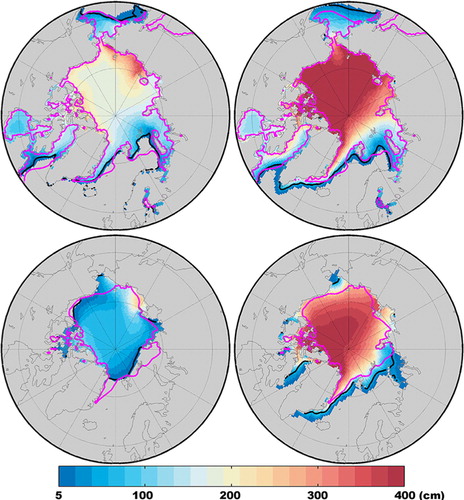
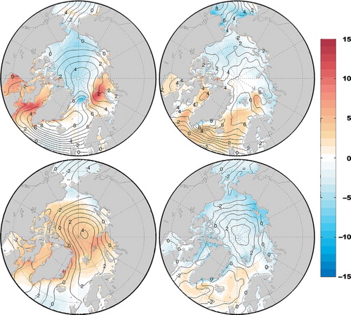
Based on numerous studies showing similar biases in the sea-ice cover and thickness distribution in coupled models (Bitz et al., 2002; DeWeaver and Bitz, 2006; Chapman and Walsh, 2007; Koldunov et al., 2010), we hypothesise that these differences mainly arise from the simulated atmosphere and associated surface forcings. This hypothesis is supported by results from Mårtensson et al. (2012) who performed RCO standalone simulations driven by ERA-40 reanalysis (Uppala et al., 2005) where the maximal sea-ice thickness is located along the CAA where present-day thickest ice is found (Bourke and Garrett, 1987; Koldunov et al., 2010). Further improvements of the sea-ice thickness distribution in Mårtensson et al. (2012) were achieved by including a multi-category sea-ice scheme which was not included in the present RCAO experiments. Moreover, Fig. 3 presents the 1980–1999 average sea level pressure (SLP) and T2M for ERA-Interim, the RCAO ensemble average, and ECHAM. In March, both models overestimate SLP over Iceland, the Nordic Seas and parts of the Atlantic sector. In September, a positive bias is centred over the Central Arctic. This bias is slightly more pronounced in RCAO than in ECHAM. The temperature difference between RCAO and ERA-Interim (Fig. 4) shows large warm bias in March over the region of underestimated sea-ice extent over the Barents and Labrador Seas, while a cold bias is present over the Central Arctic, also found in ECHAM. The bias in SLP indicates anomalous surface circulation from the CAA towards the Siberian coast in winter (not shown), which is responsible for the maximal sea-ice thickness along the Siberian coast in RCAO. This bias in ice thickness distribution associated with biases in wind forcing is a common problem in many coupled models (Bitz et al., 2002; DeWeaver and Bitz, 2006; Holland et al., 2006), and the reason for this is still poorly understood (Koldunov et al., 2010). In September, RCAO shows positive biases in SLP indicating the presence of a quasi-permanent high-pressure anomaly over Central Arctic basin with weak interannual variability within RCAO's individual projections (not shown). The biases in the SLP fields directly affect the surface winds, which in turn modify the ice dynamics. Since sea-ice drift is nearly parallel to the isobars (Kwok, 2008), the systematic high-pressure bias in RCAO compared to ERA-Interim is very likely responsible for an erroneous sea-ice motion leading to thicker sea ice along the Siberian coast. The positive T2M present in September is also likely to increase top ice melting, therefore reducing the sea-ice thickness compared to observations.

Fig. 3 1980–1999 average of T2M (colours) and sea level pressure (contours) for ERA-Interim (left), ensemble mean of the three RCAO projections (middle) and ECHAM (right) for March (top) and September (bottom).

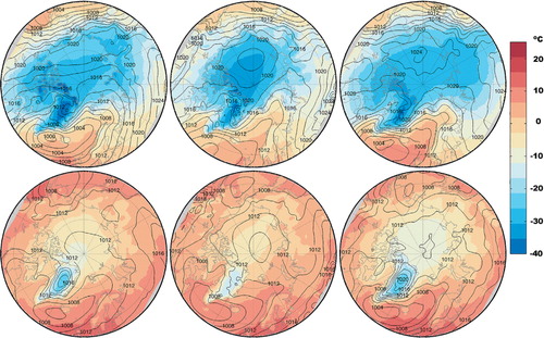
Fig. 4 1980–1999 differences for T2M (colours) and sea level pressure (contours) between RCAO minus ERA-Interim (left) and ECHAM minus Era-Interim (right) for March (top) and September (bottom).

Although ECHAM shows a similar SLP difference pattern, the maximum sea ice is located between the coast of Greenland and Ellesmere Island and the North Pole (Koldunov et al., 2010), while the overestimated thickness is most likely caused by the cold bias over the Arctic basin (Koenigk et al., 2011). Interestingly, when computed over the 2025–2044 period, sea-ice thickness distribution in ECHAM shows similar patterns to RCAO for the 1980–1999 period (not shown). Differences in sea-ice thickness and the resulting sea-ice volume between RCAO and ECHAM persist throughout the simulation, with ECHAM showing acceleration in sea-ice loss from 2020 onward (Koenigk et al., 2011).

The focus of this article is to understand the mechanisms responsible for triggering the RILEs and their effects on surface fields as simulated by RCAO, despite the model limitations. Albeit the impact of the model biases on the simulation of recent past sea-ice conditions, this study contributes to improved understanding of not only RCAO behaviour, but also of those numerous models sharing similarity in their atmospheric circulation.

4. RILEs

4.1. RILEs

In order to focus on extreme events, the RILE criteria used in this study are more conservative compared to that used in the previous study of DK. The central year of a RILE is defined when the derivative of the 5-year running mean of the minimum September sea-ice extent exceeds a value of −0.5 million km² yr⁻¹. In the case that two successive years are below this threshold, the first year is defined as the central date. The duration of each event is defined as the period around the central year showing a loss of 0.15 millionkm²yr⁻¹ or more included in a ±5-year radius. These criteria are adapted from a sea-ice loss study by H06.

Figure 5 presents the time series of the September sea-ice extent from satellite observations (Fetterer et al., 2002 [updated 2011]), simulated by ECHAM and RCAO with identification of the RILEs detected using the aforementioned criteria. First, RCAO produces realistic September sea-ice cover compared to satellite observations, although underestimated (see also Fig. 2), and the recent past decreasing trend is well captured. The driving model, ECHAM, overestimates the sea-ice cover, while it underestimates the observed decreasing trend, most likely related to the cold bias presented in Section 3.

Fig. 5 RCAO simulated September sea-ice extent is shown in black for the 1980–2080 period: ECHstand2 (top), ECHMPIstand (middle) and ECHMPIflux (bottom). Grey shadings indicate rapid ice loss events considered in this study (Table 2). ECHAM and satellite observations (Fetterer et al., 2002; updated 2011) of September sea-ice extent are presented respectively in light grey and blue on all panels.

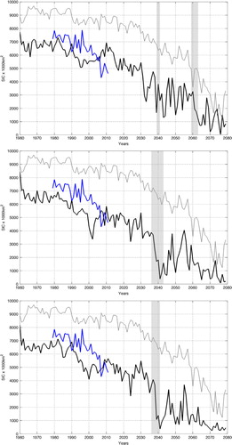
All RCAO integrations show very similar behaviour, with a decrease in the September sea-ice extent during the 1990s, recuperation in the 2000–2010 period, followed by a period of general decrease from 2010 to 2030. Between 2030 and 2040, accelerated September sea-ice loss, satisfying RILE criteria is noted. An interesting aspect is the synchronicity of the RILEs for all RCAO projections around 2040, suggesting strong control of the large-scale atmospheric boundary conditions from ECHAM (see Section 4.2.5). All projections show a partial recovery period of September sea-ice extent between 2040 and 2055, some years reaching values comparable to the sea-ice extent prior to the 2040 drastic events, followed by a third sea-ice loss period extending from 2055 to the end of the projection. The recovery is a dominant factor in the study of the impacts of RILEs by limiting the period over which the atmosphere can react to reduced ice coverage. Although ECHAM shows large negative trends in sea-ice extent from 2030 to 2080, no RILEs are detected using the aforementioned criteria in the global projection used to drive RCAO at its lateral boundaries. It should also be noted that in the study by H06 using CCSM3, sea-ice recovery was absent. A total of four RILEs in the three RCAO regional projections are considered in this study, with average duration of 5.5 yr, as summarised in Table 2.

Table 2 RILE summary

Rile identification	Projection	Central Date	Period	Length
R1	ECHstand2	2041	2039–2041	3
R2	ECHMPIstand	2039	2036–2043	8
R3	ECHMPIflux	2040	2036–2041	6
R4	ECHstand2	2063	2059–2063	5

4.2. Causes and effects of RILEs

This section investigates the characteristics of selected near-surface variables and key physical processes in action during the RILEs. Comparisons are performed between three different periods: RILE period where averages are computed over the duration of the event (refer to Table 2 for event duration) and pre-RILE period (post-RILE) where averages are computed over the 10 yr before (after) the RILE period itself. Due to the similarity of the pre-RILE and RILE periods for all the events occurring around 2040, the R2 event is presented in detail; similarities and differences with other events are discussed where appropriate.

4.2.1. Sea-ice field morphology.

Figure 6 presents bimonthly averages of sea-ice cover and thickness for the R2 event for the pre-RILE and RILE periods. For both pre-RILE and RILE periods, the Arctic ice pack in summer (July–August) and autumn (September–October) is characterised by high fractional cover extending from the East Siberian Sea shores to the CAA. In autumn, marginal seas are almost completely ice-free except the East Siberian Sea and the eastern parts of the Chukchi Sea. The thickest ice is located in the East Siberian Sea, as a result of a westward displacement of the winter high-pressure ridge over the Central Arctic Ocean, causing anomalous winds pushing the ice towards the East Siberian Sea coastal regions as presented in Section 3. This displacement is stronger during pre-RILE periods with winds parallel to the coast from the East Siberian Sea towards the New Siberian Island where ice is the thickest (not shown). This displacement is a well-known large-scale near-surface circulation bias in atmosphere-ocean coupled models (Bitz et al., 2002) accentuated by lack of sufficient number of sea-ice classes in RCAO sea-ice scheme (Mårtensson et al., 2012). A secondary maximum is located along the CAA shore at the location of present-day thickest ice (Bourke and Garrett, 1987).

Fig. 6 Bimonthly averages of (a) sea-ice cover (fraction) and (b) thickness (cm) for pre-RILE (top) and RILE (bottom) period for R2 (2039 event, projection ECHMPIstand).

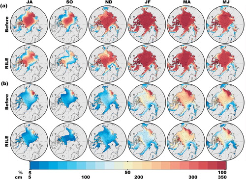
The largest differences in the sea-ice cover between pre-RILE and RILE periods are noted for the September–October period. Sea-ice cover fraction decreases over the whole Arctic ice pack, and open water is formed principally in two distinct regions, over the Canada basin and in the vicinity of the North Pole.

Although the maximal sea-ice loss occurs in late autumn, changes can be noted in the sea-ice cover in early winter (i.e. November–December) suggesting a delay in the formation of new ice due to accumulation of heat in the ocean. The regions that show decreasing sea-ice fraction are along the marginal ice zone in the Atlantic sector (in the vicinity of Franz Joseph Land) and offshore of East Siberian Sea towards Chukchi Sea and extending weakly to Beaufort Sea. During the RILE period, signs of early melt in summer (July–August) are visible along the coast of Alaska and in the Atlantic sector along the ice marginal zones, potentially contributing to accelerated ice melt during late summer, as suggested in Steele et al. (2010). The Arctic ice pack is characterised by thin ice (<1m) over Central Arctic in the pre-RILE and RILE periods, suggesting high potential sensitivity of the sea-ice cover to external factors such as modification in the large-scale atmospheric and oceanic circulations or changes in surface energy budget, presented in detail later in this study.

4.2.2. Sea-ice vulnerability and long-term pre-conditioning by thinning.

Observations and numerical experiments suggest that long-term thinning of the Arctic ice plays a major role in increasing the ice vulnerability to external forcing such as changes in large-scale atmospheric and oceanic circulations, changes in radiative fluxes or surface temperatures (Holland et al., 2008; Kay et al., 2008; Perovich et al., 2008). This increased vulnerability is believed to have led to the 2007 minimum in sea-ice cover. Figure 7a presents the evolution of average September sea-ice thickness for the Arctic for the 1980–2070 period calculated over each grid point where sea-ice cover is larger than 15%. Decreasing trend is clearly visible over the 1980–2040 period, in good correlation with the September sea-ice extent (Fig. 5).

Fig. 7 (a) Average September sea-ice thickness for ECHStand2 (blue), ECHMPIStand (red), ECHMPIFlux (green) and ensemble average (black). (b) Relation between 20-year standard deviation of September sea-ice extent to 20-year average sea-ice thickness. Dots are used for 1980–2040 period, while diamonds corresponds to the 2041–2070 period. Black symbols represent the ensemble average of the three simulations.

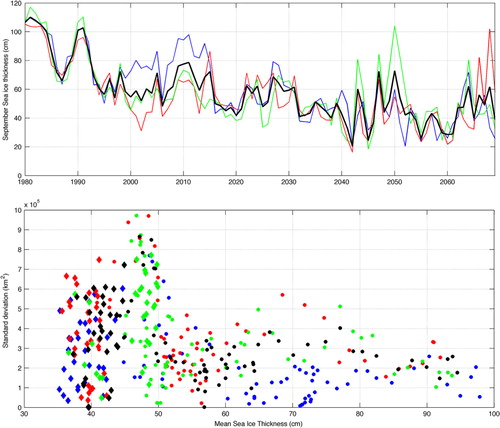
To evaluate the vulnerability of the sea-ice extent to the thinning of the ice, Fig. 7b presents the relationship between the standard deviation of September sea-ice extent and the average sea-ice thickness for 20-year sliding windows over the 1980–2070 period. The standard deviation of September sea-ice extent is computed using each regional projection after subtracting the ensemble average. In this way, we measure the natural variability in September sea-ice extent of each simulation excluding the large-scale signal, filtered in the ensemble average. The small number of projections is compensated by the synchronicity of the events allowing reasonable removal of the large-scale signal. As shown in Figs. 2 and 7b, RCAO generally produces thinner ice compared to other climate models (Holland et al., 2006, 2008, 2010; Koenigk et al., 2011), with Arctic Basin maximum average September thickness reaching at most 120cm in the 1980s (Fig. 7a). Nevertheless, Fig. 7b confirms increased variability of September sea-ice extent for thinner ice for all projections and for the ensemble mean. Compared to a similar plot in the study of Holland et al. (2008) where asymptotic behaviour was clearly visible with decreasing variability at thickness below 1m, RCAO shows very large variability even in very thin ice conditions (<50cm), suggesting that ice formation is highly sensitive to interannual changes of the exterior factors such as large-scale atmospheric and oceanic flows or changes in radiative fluxes, explored later in this study.

4.2.3. Changes to selected near-surface fields during RILEs.

Changes in sea-ice cover and thickness modify the surface conditions seen by the atmosphere. Figure 8a shows bimonthly differences between the RILE and the pre-RILE periods for sea-ice cover and thickness. Maximal ice thickness reduction during the RILE occurs in September–October over the East Siberian Sea causing a sea-ice cover reduction from 90–95% to 75%. The Central Arctic also thins from 50cm down to 15cm around 150°E, leading to a sea-ice cover decrease from 80 to 50%. November–December shows similar thinning pattern and magnitude as September–October (Fig. 8a) but the ice is thick enough to effectively cover most of the Arctic Basin, causing small changes in the sea-ice cover. The T2M increases during late autumn (September–October) but the maximal warming, up to 10°C, occurs over the ocean during early winter (November–December). Statistical analysis of the T2M differences between the pre-RILE and the RILE periods was performed using a t-test at 80, 90, 95 and 99% confidence levels (Fig. 8a). The 100-year trend in T2M was removed prior to the testing to isolate the effect of the event from the background warming. Despite the limited length of 10 yr for the pre-RILE period and 8 yr for the RILE period, Fig. 8a shows that the warming is mostly significant over the 95% confidence level for the Central Arctic Ocean during late autumn and winter. The warming patterns over the Nordic Seas in September–October are also significant above 90% which will be shown later in this study to be crucial in the understanding of the RILE mechanism for the Atlantic Sector of the domain. In MJ and JA, the large area of statistical significance over the Arctic Ocean and the weak signal in the trended differences is simply caused by a compensation between the long-term warming trends and a short-term decrease in temperatures between the two periods over these months in the detrended fields. While the detrended differences are small, between −2 and 0°C, the very small interannual variability of the temperature reaches statistical significance. In the non-detrended differences, there is a net compensation between the long-term warming trends and the short-term cooling leaving an almost zero signal in the differences.

Fig. 8 (a) Bimonthly differences of RILE-(Pre-RILE) averages for R2 event: sea-ice cover (SIC,%), sea-ice thickness (SIT, cm), T2M (T2m, °C) and statistical significance of the T2M following a t-test at significance levels: 80%-blue, 90%-green, 95%-yellow and 99%-red. The 100-year trend in T2M was removed prior to statistical significance testing. (b) same as Fig. 8a but for: surface net radiative balance (Q_net, Wm²), combined latent and sensible heat fluxes (LHF+SHF, Wm⁻²), net surface longwave (LW_net, Wm⁻²), and net surface shortwave (Q_net, Wm⁻²). Fluxes are defined negative upward (away from the surface).

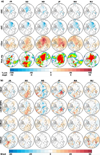
It is found that the T2M response follows the changes in the net surface energy budget, and not the maximal changes in sea-ice cover (Fig. 8b). The delay between the maximal increase in air temperature relative to the sea-ice cover during the RILE period can be explained by increases in the turbulent heat fluxes, both sensible and latent, during the November–December period. Differences are due to the greater exposure of ice-free ocean to colder surface air temperature in early winter compared to milder autumn air temperatures. The radiative contribution to the changes in net surface energy budget is limited to −5Wm⁻² for terrestrial radiation while solar contribution is zero during the polar night (Fig. 8b).

The January–February maximal warming is located at the sea-ice margin of the Atlantic sector and over the Kara Sea. Both regions show statistically significant warming caused by the increase in the surface turbulent fluxes due to sea-ice retreat. Increased anomalies in turbulent fluxes towards the atmosphere are located over retreating sea-ice margin, caused by increased exposure of the atmosphere to the relatively warm ocean causing a northward shift in the location of the maximum ocean-atmosphere heat transfer. The region of decreased ocean heat loss over the Barents Sea (Fig. 8b) is partly caused by the anomalous southerly circulation over the area, discussed in detail in the next section, decreasing the ocean-atmosphere vertical temperature gradient, thus reducing heat transfer. This dipole structure, consisting of decreased-increased ocean-atmosphere heat fluxes along the retreating sea-ice margin, is coherent with results from CAM3 simulations analysing the effect of imposed reduction of sea-ice cover during a hindcast experiment (Deser et al., 2010).

The net surface solar radiation (Fig. 8b) increases due to the retreat of sea ice in May–June over the Kara Sea (30–35Wm⁻²) and Northern Baffin Bay. This increased absorption of solar radiation, mostly by open water, warms the ocean surface layer and increases the heat content of the ocean, potentially used for bottom ice melt, as suggested by many observations and modelling studies (Kay et al., 2008; Perovich et al., 2008; Steele et al., 2010). The role of increased absorbed solar radiation by the ocean before and during the RILE is found to be a dominant factor over the Pacific sector of the Arctic Ocean in RCAO and are presented in the next section.

The R1 and R3 events resemble the R2 event in multiple aspects. The R3 event (ECHMPIflux) shows stronger sea-ice loss for all seasons, with a broader zone of thinning covering the entire Arctic ice pack in September–October and also larger loss in the marginal ice zones of the North Atlantic sector for all other seasons. The spatial patterns of increase/decrease of the T2M for R3 are slightly different when compared to the R2 event. Nevertheless, they are caused by the same mechanisms, i.e. changes in the net surface energy flux with the turbulent fluxes playing a dominant role in autumn and winter, while increase in net shortwave is important in spring.

The sea-ice cover differences are smaller for R1, especially in the marginal ice zones of the North Atlantic sector, leading to milder changes in T2Ms and energy fluxes. This is linked to the oceanic heat transport and is explained in detail in Section 4.2.5. The R4 event occurs in 2063, nearly 20-yr after the first period where the R1, R2 and R3 events occur (~2040) and after the sea-ice ‘recovery’ of the 2050s. Therefore, sea ice is thinner and likely increases the sensitivity of the ice to changes in atmospheric fluxes or changes in circulation. Nevertheless, patterns for both sea-ice cover and thickness and their changes during the RILE are similar to the 2040 events and shows similar changes to the surface energy fluxes.

4.2.4. Large-scale atmospheric circulation and SST anomalies.

The general circulation patterns present in the decades preceding the RILEs (2020–2040) are very similar to those of the 1980–1999 climatological period presented in Section 3. Both RCAO and ECHAM show continuity in the large-scale atmospheric patterns, suggesting a small sensitivity of the atmospheric large-scale circulation to the increased GHG concentrations. Therefore, the analysis of the anomalies in the large-scale circulation causing the RILEs is performed in the context of quasi-permanent anticyclonic circulation over the Arctic basin with relatively weak interannual variability.

In this section, the impact of the short-term modifications of the large-scale atmospheric circulation and SSTs is analysed. Figure 9 presents bimonthly anomalies of sea-level pressure (SLP) and SST between the RILE and the pre-RILE periods for the R2 event along with an analysis of the statistical significance of the differences using a t-test.

Fig. 9 Bimonthly differences of RILE-(Pre-RILE) averages for R2 event sea level pressure (first row), sea surface temperature (thirrd row) and their statistical significance (second and fourth row). In the figure showing the statistical significance, blue, green, yellow and red correspond to 80, 90, 95 and 99% confidence levels.

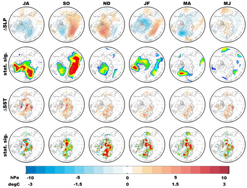
In July and August (JA), the SST increase over the entire Atlantic sector of the domain, defined as the region between the Nordic Seas extending to the Lomonosov ridge. While the warming is moderate over the Nordic Seas (0.3–0.6°C) the northernmost region shows statistical significant warming. Larger warming, up to 3°C, can be noted over the Kara Sea and along the retreating sea-ice margin near the North Pole with statistical significance over the 90% confidence level. Maximal SST warming for JA is collocated with maximum increases in T2M and sea-ice loss (Fig. 8a) near the North Pole, the southern regions being already ice-free in the pre-RILE period.

In September–October, positive SST anomalies, though reduced in magnitude, are still present and statistically significant at 95% over regions where sea-ice cover decrease has been noted, namely near the North Pole and offshore of the East Siberian Sea (Fig. 8a). The SST over those regions remains above freezing point (not shown) thus delaying sea-ice formation. The statistically significant SLP anomalies in autumn (Fig. 9) lead to anomalous southerly winds, advecting warmer air from the Nordic Seas towards the Arctic. Conjointly, changes in T2M over the same region are also significant. One can clearly see a downward net surface energy flux anomaly (Fig. 8b) over broad region of the Barents Sea, resulting from a decreased air-ocean temperature contrast caused by the advection of warmer air from the south. This decrease in the energy flux from the ocean to the atmosphere slows the cooling of the near-surface ocean layers, allowing for the warm anomaly to persist, penetrate deeper in the Arctic region, and further delay the ice formation. Warm atmospheric inflow in that region during RILEs is coherent with similar finding for summer (JAS) in DK.

During early winter, i.e. November–December, positive SST anomaly is still present and significant in the North Atlantic sector but in a reduced amplitude due to the change in the anomalous large-scale atmospheric circulation. Indeed, the positive SLP anomaly south of Iceland in November–December signals a weaker Icelandic low-pressure system, thus reducing heat transport from the North Atlantic towards the Arctic. Deprived of heat advection from the southern flow, the atmosphere cools rapidly increasing ocean-air temperature gradient at the surface. This leads to increased turbulent surface fluxes in the North Pole region (Fig. 8b) and thereby increasing the surface cooling in the ocean producing favourable conditions for the onset of ice formation.

In January–February, changes in the SLP anomaly show a regain of wind blowing from lower latitudes, directed towards the Barents Sea. The advection of warmer air over Barents Sea decreases the air-ocean temperature gradient, causing downward net energy flux over most of the region, except the location of sea-ice loss, where strong upward fluxes are observed (Fig. 8b). Again, net downward fluxes cause the positive SST anomaly to persist and to remain statistically significant.

While March–April SLP shows a deeper cyclonic Icelandic system during the RILE period, the circulation anomaly is mainly located over the Nordic Seas and does not propagate as far north as it did for January–February and September–October. This results in decreased amplitude of T2M and net radiative balance anomalies over the Barents Sea (Fig. 8b). In May–June, significant positive SST anomalies develop over the regions of decreased sea-ice cover although the SLP anomalies do not suggest southerly inflows. The positive SST anomaly is shown to be caused by the increased net shortwave absorption of 30Wm⁻² along the sea-ice margin, reaching value of 40Wm⁻² over the Kara Sea, which increases the ocean heat content near the surface, explaining large positive SST anomalies in the following months.

For the Pacific sector, Woodgate et al. (2010) showed an increase in the observed oceanic heat transport from the Northern Pacific to the Arctic through Bering Strait. They suggest that this increased heat acts as a trigger for the early onset of sea-ice melt. These results are supported by the modelling experiment of Steele et al. (2010), where early melt along the Alaska coast is reported to be caused by the increased Bering Strait inflow, leading to the 2007 minimum. In RCAO, Ekman convergence in the ocean, resulting from the quasi-permanent anticyclonic circulation presented in Section 3, greatly reduces the Bering Strait inflow by creating a broad region of increased sea surface height (SSH) covering most of the Arctic basin (not shown). The above, along with the presence of a closed ocean lateral boundary located along the Aleutian Islands, precluding exchange with the North Pacific, leads to underestimation of the Bering Strait inflow in RCAO. In the absence of significant changes to the Bering Strait inflow during RILEs (not shown) and limited vertical heat transport from deeper ocean towards the surface (DK), other mechanisms causing the large sea-ice melt over the Pacific sector were investigated. Perovich et al. (2008) showed that the increase of absorbed solar radiation by the ocean played a major role in the negative sea-ice mass balance observed for the 2007 minimum, by triggering a sea-ice albedo feedback that contributed to the accelerated the sea-ice retreat.

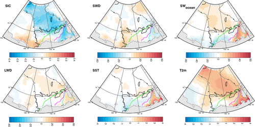
Figure 10 shows the averaged anomalies of surface sea-ice conditions, radiative fluxes, SST and T2M computed over the period from May to October (MJJASO) between the year of minimum sea-ice cover for event R2 (2041) and the 2010-2030 average. Sea-ice cover shows strong decrease over the Beaufort Sea with signs of retreating sea-ice margin (SIC>15%) initialised from the Amundsen Gulf in May (contours in Fig. 10), evolving towards an ice-free region along the Alaska coast in August (green curve). The early sea-ice retreat is triggered by anomalous sea-ice velocity from the coast towards central Beaufort Sea (not shown). This retreat reaches a maximum in September (grey curve), where open water is present over most of the Beaufort Sea, leading to large negative SIC anomaly. Downwelling shortwave radiation at the surface shows average negative anomalies over the retreating sea-ice margin in southwestern Beaufort Sea, caused by the increase in the low cloud cover (not shown) resulting from the presence of more open water associated with release of moisture from the ocean to the atmosphere. Nevertheless, the absorbed shortwave radiation by the open water shows strong increase over the same region reaching averaged monthly values of 30Wm⁻² (45Wm⁻² in May–June). This increased energy absorbed by the ocean leads to a warming of SSTs by up to 3°C. The combination of early sea-ice retreat, increased solar energy absorbed by the ocean and an ocean circulation directed from the coastal region towards the retreating ice edge strengthens the sea-ice albedo feedback and accelerates the bottom melt of the remaining thin ice present over the region. The contribution from downwelling long-wave radiation (Fig. 10) is smaller over the entire Beaufort Sea with maximum values less than 5Wm⁻² over the southwestern Beaufort Sea. The increased in downwelling long-wave radiation corresponds to the near-surface temperature, resulting from the presence of open water and increased heat transfer from the ocean to the atmosphere. The increased T2M over the Northern Beaufort Sea is the result of summertime advection from the Atlantic sector, enhancing top melting of the sea-ice over the area, where little changes are observed in both downwelling short-wave and long-wave radiation at the surface. Compared to observations of the 2007 event (Kay et al., 2008; Perovich et al., 2008), the simulated sea ice present over the Pacific sector in RCAO is much thinner increasing its sensitivity to smaller perturbations in the radiation and clouds.

Fig. 10 Average MJJASO anomalies between 2041 against the 2010-2030 period for: sea-ice cover (top left), short-wave radiation down at the surface (top middle), shortwave radiation absorbed by the ocean (top right), long-wave radiation down at the surface (bottom left), sea surface temperature (bottom middle) and T2M (bottom right). Radiative flux anomalies are presented in Wm⁻² and temperatures anomalies in °C. Contours show the location of the 2041 sea-ice margin (sea-ice cover>15%) for June (yellow), July (cyan), August (green), September (grey) and October (black).

4.2.5. Synchronicity of RILE events and ocean heat transport contribution.

The synchronicity of the RILEs during the regional climate projections, with three of the four events occurring around 2040 (Fig. 5), suggests a strong control of the large-scale atmospheric and oceanic circulation on the timing of the events. Figure 11 presents a comparison of the 850hPa geopotential heights anomaly between 2036 and 2042 encompassing the first three RILEs and the prior 10-year period (2026–2035). Figure 11 shows the differences between those time periods for the ECHAM climate projection used to provide the atmospheric lateral boundary conditions to all three RCAO projections along with an estimation of the statistical significance using a t-test. The 850hPa geopotential height field allows evaluation of lower tropospheric circulation, while limiting the effect of surface processes.

Fig. 11 Changes in 850hPa geopotential height for March–April (first row), statistical significance (second row), September–October (third row) and its statistical significance (fourth row) between period around RILEs (2036–2042) and the preceding 10-year period (2026–2035) for the driving model ECHAM, RCAO events R1, R2 and R3, from left to right respectively. In the figure showing the statistical significance from a t-test, blue, green, yellow and red correspond to 80, 90, 95 and 99% confidence levels. The last column represents the standard deviation amongst RCAO for the three projections.

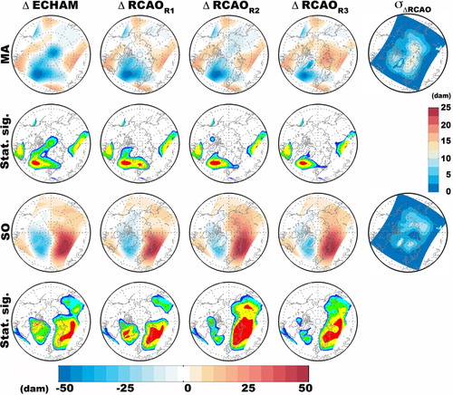
The comparison of the anomaly for ECHAM and the three RCAO regional projections shows large consistency between the four patterns for both the March–April and September–October periods, especially along RCAO lateral boundaries. As expected, differences between ECHAM and the regional projections and amongst individual regional projections grow towards the central part of the domain showing the decreased influence of the lateral boundary conditions towards the central part of the domain. Nevertheless, all regional projections show statistically significant geopotential anomalies leading to increased advection from the Nordic Seas towards the Central Arctic Ocean in September–October and a deepening and northward extension of the Icelandic low in March–April. These results support the hypothesis of increased heat transport from the Nordic Seas towards the Arctic during the RILE periods. Over the North Atlantic sector, one can notice that the amplitude of the geopotential height is, over most of the region, one order of magnitude larger compared to the standard deviation of the difference amongst the regional projections. The large values of the geopotential height anomalies compared to the variability amongst individual projections, their similarity compared to ECHAM, and the high level of statistical significance of the signal rule out the possibility that these anomalies occur randomly within RCAO projections. Moreover, the results presented in Fig. 11 can be generalised over the annual cycle and for multiple vertical levels in the atmosphere (not shown), again reinforcing the conclusion that the anomaly propagates from the common lateral boundary conditions provided by ECHAM.

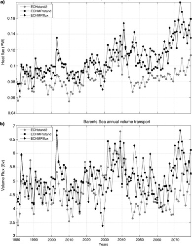
Patterns of large-scale atmospheric circulation in events R1, R2 and R3 show anomalous winds from Nordic Seas towards the polar region. These winds generate positive anomalies in the annual oceanic heat transport (OHT) reaching the Barents Sea shelf (Fig. 12). Barents Sea OHT is computed over the first 290m of the ocean (top 25 vertical levels) along a transect from Svalbard to the Kola Peninsula using a reference temperature of −0.1°C. OHT in the Barents Sea shows an increase for all RCAO projections from 2010 reaching maximum values around 2040, the central dates of R1, R2 and R3 events. The large increase from 2030 to 2040 is caused by a combination of warmer water and increased volume transport through the section, contributing to the SST warming observed over the Barents Sea during the RILE events (Fig. 9). The differences in OHT between ECHstand2 (R1) and the other two projections increase after the 2040 maximum. The OHT simulated by the ECHStand2, which uses repeated climatological ocean lateral boundary conditions, decreases abruptly after 2040 reaching a minimum in 2045, followed by moderate increase until the end of the projection. However, the other two projections using ocean lateral boundary conditions from the global model scenario, responsible for the R2 and R3 events, show smaller decrease in OHT after 2040. It suggests that the OHT decrease in ECHMPIstand2 is responsible for a milder R1 event with reduced magnitude and duration compared to R2 and R3 events. The differences in the ocean lateral boundary condition cause the ECHstand2 to generate a more diffuse and warmer North Atlantic sub-polar gyre while the ECHMPIstand and ECHMPIflux favour warmer and stronger inflow along Ireland causing a warmer and more intense Norwegian Current which penetrates further North (not shown) causing increased temperatures in the Nordic Seas and in the Barents Sea for those two runs.

Fig. 12 Time series of the Barents Sea opening annual (a) oceanic heat transport (PW) and (b) volume transport (Sv) computed using a reference temperature of −0.1°C over the first 290 model first 25 vertical levels) for three RCAO climate projections: ECHstand2 (grey line), ECHMPIstand (black full line) and ECHMPIflux (black dotted line).

The results presented in this section lead the authors to comfortably conclude that the synchronicity of the RILE events is caused by anomalous large-scale atmospheric circulation propagating from the driving model ECHAM, efficiently propagating from the lateral boundary conditions in the North Atlantic into the regional projections. This anomaly causes increased atmospheric and oceanic heat transport towards the Arctic Ocean, contributing to important sea-ice reduction.

4.3. Impacts of RILEs

This section investigates the effects of the RILEs on the post-RILE period from different aspects: variability, changes over coastal regions around the Arctic Ocean and the atmospheric vertical structure.

4.3.1 Post-RILE variability.

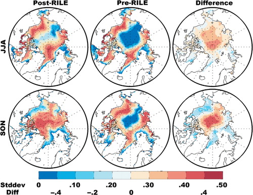
Following the events R2 and R3, a partial recovery period is seen in September sea-ice extent (Fig. 5), also characterised by increased interrannual variability. The high variability at low sea-ice thickness (Fig. 7) suggests the ability of the model to easily form thin ice, sufficient to cover relatively large areas of the Arctic Ocean. To illustrate the changes in the spatial distribution of ice and its variability, seasonal standard deviation is computed over the pre-RILE and post-RILE periods for all events. The respective linear trends for each period were subtracted prior to calculating the standard deviation. Figure 13 presents results for the R2 event; similar conclusions are valid for R3 and R4 events, while R1 shows weaker changes due to the smaller amplitude of the event. In summer and autumn, a transition towards a more variable ice pack is observed from pre-RILE to post-RILE period. While a stable Arctic ice pack was present in summer during the pre-RILE period, represented by the area of low interrannual variability extending from the East Siberian Sea coast towards Central Arctic, very little of it remains after the RILE except over narrow regions of the East Siberian Sea and the CAA. In autumn, the annually present ice pack completely disappears. This is caused by a transition in the sea-ice extent towards a more chaotic behaviour with high sensitivity to anomalies in surface forcings and atmospheric circulation. Increased variability in the sea-ice extent is not present in CCSM3, where September sea-ice standard deviation is shown to peak during the RILE to rapidly decrease in the years following the event (see Fig. 3c and Plate 5 in H08).

Fig. 13 Summer and autumn seasonal standard deviation of sea-ice cover for post-RILE (left), pre-RILE (middle) and their differences (right) for R2 event.

4.3.2. Atmospheric and land response.

To determine the longer term changes caused by the rapid decrease of sea-ice cover, Fig. 14 shows the average temperature anomaly for the R2 event, relative to the pre-RILE conditions, for both the RILE and the post-RILE periods over the Arctic Ocean and the surrounding continental areas. Coherently with the bimonthly temperature changes (Fig. 8), the warming is maximal over the ocean in December (5.2°C), mainly caused by the increased turbulent fluxes over remaining open water, and minimum (0.4°C) in May. Important consistency is found between the annual cycle of the temperature anomalies for the two periods over ocean and land. Warming over land shows the same annual cycle as that over the ocean but with smaller amplitude, with increases of 3.3 and 1.3°C for December and May, respectively. The similarity between the annual cycle of the temperature anomalies for the RILE and post-RILE periods, generally 0.5°C apart, shows a transition towards warmer climate despite the relative recuperation of the sea-ice cover in the post-RILE period. This is probably caused by the low thickness of the ice incapable of effectively insulating the atmosphere from the ocean combined with the general warming trend likely caused by increased GHG concentration, since most of the warming over land is not statistically significant when the 100-year trend is removed (Fig. 8a).

Fig. 14 T2M differences for RILE minus Pre-RILE periods (dark colours) and Post-RILE minus Pre-RILE (light colours) over the Arctic Ocean (top left), Arctic Land (bottom left), Siberian Sea (top right) and Siberian Land (bottom right). Arctic land is defined between 45–290°E and between 65°N and the coast while the Siberian sector is defined between 110–190°E and 65–90°N.

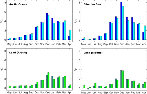
The T2M response during the event (Fig. 8) showed maximum increases in temperatures over the East Siberian Sea in November–December caused by a delay in the ice formation over that region. The regional maximum warming is clearly visible over the Siberian Sea sector, defined between 110–190°E and 65–90°N (Fig. 14) with warming from 7.2 to 8.1°C in December, 3°C larger compared to the average Arctic Ocean warming. Despite the increased ocean warming over the East Siberian Sea, the nearby coastal area between 110 and 190°N and from 65°N to the coast shows smaller response with increases of 3.7°C, corresponding to increased warming between 0.4 and 1°C compared to Arctic Land.

Nevertheless, one would expect the warmer air present over the ocean to be advected over land by the anticyclonic circulation over the region (not shown). The rapid attenuation of the warming over land raises the question of the atmospheric heat transport mechanism, which is addressed in the next section.

4.3.3. Impact of RILEs on atmospheric structure.

One would expect near-surface horizontal propagation of the warming signal due to the strong atmospheric stability caused by the Arctic low-level inversion. Studies by Deser et al. (2010) and Lawrence et al. (2008) showed propagation of a more uniform latitudinal warming over the continent, penetrating up to 1500km inland, a signal very different in RCAO projections (Figs. 8 and 14).

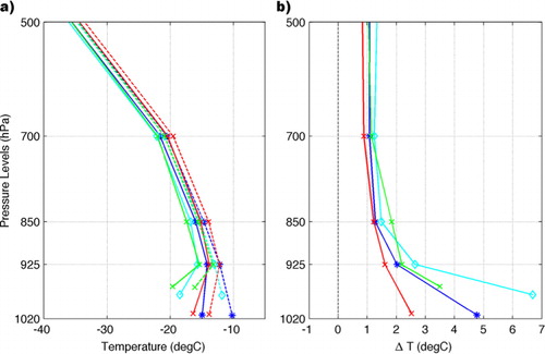
To understand the propagation of the warming signal, a comparison of spatially averaged November–December vertical temperature profiles for pre-RILE and RILE periods as simulated by RCAO is presented in Fig. 15. Very weak low-level temperature inversion is noted from the profiles over the Arctic Ocean for both pre-RILE and RILE periods (~1°C). Inversions of 2.8 and 4.2°C are visible in the pre-RILE profiles for the East Siberian Sea and nearby land respectively, limited between the surface and 925hPa. The Siberian Sea inversion disappears during RILE, while the Siberian land inversion is reduced to 2.8°C. While the warming signal is, as expected, strongest near the surface, temperature increases in the vertical, reaching heights of 500hPa and above. This indicates an equivalent-barotropic structure to the warm anomaly; such structure is as expected associated with rather weak horizontal transport of heat from the oceanic region towards the continent. In present-day observations, strong linear relation has been demonstrated between the low-level inversion strength and the density of the underlying sea-ice cover (Pavelsky et al., 2011). It is very likely that in the transient RCAO climate projections, the progressive decrease in the sea-ice cover and thickness leads to gradual erosion of the atmospheric inversion. This reduced atmospheric stability might explain the vertical propagation of the surface warming during the events, therefore reducing their effects on surrounding continental areas.

Fig. 15 November–December (a) spatially averaged vertical temperature profile over Arctic Ocean (blue), Siberian Sea (cyan), pan-Arctic land (red) and Siberian Sea land sector (green) for Pre-RILE (full) and RILE periods (dotted). (b) Differences RILE-(Pre-RILE) for same regions. The Arctic Ocean here is the region between latitudes 80–90°N between 90°W to 60°E and from 68–90°N from 60°E to 90°W. The Siberian Sea covers longitudes between 110°E to 190°E from the coastline to 90°N, while the Siberian Land covers land from 60°N to the coastline.

5. Discussion and conclusions

The regional climate projections performed using the Rossby Center Atmosphere-Ocean modelling system produced four RILEs within three transient climate projections. The clustering of the major sea-ice loss events around 2040 is caused by the combined effects of long-term sea-ice thinning and large-scale atmospheric and oceanic circulation anomalies originating from the common ECHAM lateral boundary conditions used to drive all three RCAO projections. The anomalous atmospheric and ocean northward flow causes increased heat transport from the Nordic Seas towards the Arctic region. The increased heat transport reaching the Barents Sea Shelf causes sea-ice reduction over the Barents Sea and in the vicinity of the North Pole. Similar mechanisms were suggested by Francis and Hunter (2007) based on observations and by H08 using results from CCSM3.

Although the maximal changes in the sea-ice cover occur in September, changes in surface variables are maximal during early winter (November–December) and are driven by the changes in the net energy flux. The net energy flux is mainly influenced by the increase in the turbulent latent and sensible heat fluxes. Compared to the more idealised study of Deser et al. (2010), results obtained in RCAO transient climate projections show more moderate changes in most of the atmospheric variables, especially the erosion of the Arctic wintertime inversion, the precipitation, and the snow cover (not shown). Nevertheless, the temporal changes in the surface energy fluxes are in good agreement with that of Deser et al. (2010), showing similar seasonality and comparable mechanisms albeit the differences in the spatial patterns.

Over Beaufort Sea, a sea-ice albedo feedback occurs over the retreating sea-ice marginal zones. This sea-ice albedo feedback is triggered by anomalous circulation pushing the ice from the coastal areas towards the centre of the Beaufort Sea, causing an increase in the absorption of solar radiation by the ocean. The increase in the energy absorbed by the ocean causes an increase in the SSTs and bottom melting along the retreating sea-ice margin. Although anomalies in surface fluxes are weaker compared to the observation during the sea-ice minimum of 2007 (Kay et al., 2008), the presence of thin ice in RCAO allowed large sea-ice cover reduction despite the smaller anomalies simulated in the surface radiative fluxes.

RCAO shows increased variability in the sea-ice cover after the RILEs. This result strongly suggests an increased sensitivity of the sea-ice cover to changes in the large-scale atmospheric circulation and the surface radiative fluxes, leading to the partial recovery period observed during the post-RILE period. Despite the increased post-RILE sea-ice cover variability, both in space and time, the T2M shows signs of a transition from colder pre-RILE to generally warmer post-RILE. This transition present over the Arctic Ocean and peripheral land areas suggests decreased control of the sea-ice cover on atmospheric variables potentially due to reduced insulation efficiency of thin sea ice.

The differences in the geographic location of the temperature changes between RILEs show a strong relationship between the regional response and the location of sea ice in RCAO. Lawrence et al. (2008) showed maximum warming over land in the CAA region while R2 event shows maximum differences over Oriental Siberia, caused by the maximum decrease in sea-ice cover and thickness occurring upwind of that specific location in this particular event. Moreover, event R3, with maximal sea-ice loss in the vicinity of the North Pole showed very little impact on land simply because the warm anomaly was advected southward toward the Greenland Sea, influencing no land masses along its path. The limited impact on land is caused by the vertical propagation of the surface heat anomaly rather than horizontal, caused by the absence of low-level temperature inversion over the ocean. Previous studies during recent-past, showed strong relation between the inversion strength and the sea-ice cover but in the context of a transient climate change experiment, it is likely that the progressive thinning of the ice causes decreased surface cooling that gradually erodes the inversion.

It has been shown that RCAO sea-ice cover and thickness suffers from relatively large biases in the atmospheric large-scale circulation over the Central Arctic basin caused by a quasi-permanent anticyclonic gyre combined with underestimation of its interannual variability. This bias in the sea-level pressure, present in many coupled climate models, causes erroneous surface forcing acting on the sea ice and is responsible for the displacement of the maximum sea-ice thickness towards the Siberian coast. The causes for this artificial anticyclonic circulation over the Arctic basin in numerical models are still poorly understood at this point. Furthermore, the stability of the anticyclonic circulation throughout the RCAO climate projection tends to generate large region of positive SSH anomaly over the Arctic, decreasing the gradient between the Bering and Beaufort Sea, therefore reducing the Bering Strait inflow (not shown). Studies of the 2007 event showed that increased heat transport through the Bering Strait (Woodgate et al., 2010) was a factor in triggering the early sea-ice retreat along the Alaska coast, most likely allowing the onset of sea-ice albedo feedback (Steele et al., 2010). The underestimation of Bering Strait inflow in RCAO limits the ability of the ocean to produce RILEs originating from the Pacific sector of the Arctic Ocean, explaining the ‘Atlantic origin’ of the events presented in this study. However, the 2012 September sea-ice minimum was related to large sea-ice reduction both in the Pacific and Atlantic sectors, indicating RILEs with ‘Atlantic origin’ are possible and their analysis relevant.

Compared to observations, to ECHAM, and other modelling studies, RCAO produces thinner ice for the recent past period (1980–1999), most likely increasing the vulnerability of the modelled ice pack to changes in large-scale forcings and changes in the radiative fluxes, especially after decades of warming due to the increase in GHG concentration.

The ECHAM realisation used to provide the atmospheric (and oceanic) lateral boundary conditions shares similar large-scale atmospheric circulation biases. This circulation anomaly, combined with the cold biases in ECHAM climatology explains the overestimated sea-ice volume compared to observations and the large difference in sea-ice volume compared to RCAO throughout the climate projections (Koenigk et al., 2011). Despite very similar large-scale atmospheric anomalies in ECHAM propagating into RCAO, the presence of thicker ice in ECHAM most likely decreases the sea-ice vulnerability. This explains the absence of the 2040–2055 RILEs in ECHAM.

This study confirms that large-scale atmospheric anomaly is a key element for triggering RILEs in RCAO projections combined with the pre-conditioning by long-term thinning of the sea ice. These results strengthen the conclusions found in DK, based on a much broader range of events of smaller amplitude. Moreover, it demonstrates the strong control of the driving GCM on the timing and synchronicity of RILEs. Future work is required to address this issue more thoroughly by performing ensemble of simulations driven by several GCMs at RCAO atmospheric and oceanic lateral boundaries. This will help assess the relative role of the driving model on RCAO solutions over the Arctic region. In-depth analysis of this relevant aspect will be possible within the framework of the Coordinated Regional Downscaling Experiment, CORDEX, that is presently underway with RCAO as one of the participating models (http://www.meteo.unican.es/en/projects/CORDEX).

Acknowledgements

The authors thank Prof. René Laprise for constructive discussion and comments on this article. Thanks are also due to the members of Rossby Centre and Per Pemberton at Stockholm University for their support and discussions. The authors thank the two anonymous reviewers for constructive comments that allowed improvements to this article.

This research was undertaken within the framework of a Collaborative Research and Development project funded jointly by Natural Sciences and Engineering Research Council (NSERC) of Canada, Hydro-Québec and Ouranos consortium. The first author was also partially funded by the ‘Fonds de recherche du Québec, Nature et Technologies (FQRNT)’.

References

- Arctic Climate Impact Assessment (ACIA). Arctic Climate Impact Assessment. 2005. Cambridge University Press, Cambridge, UK,.
- Bitz C. M , Fyfe J. C , Flato G. M . Sea ice response to wind forcing from AMIP models. J. Clim. 2002; 15: 522–536.
- Bourke R. H , Garrett R. P . Sea ice thickness distribution in the Arctic Ocean. Cold Regions Sci. Technol. 1987; 13: 259–280.
- Chapman W. L , Walsh J. E . Simulations of Arctic temperature and pressure by global coupled models. J. Clim. 2007; 20: 609–632.
- Collins W. D , Bitz C. M , Blackmon M. L , Bonan G. B , Bretherton C. S , co-authors . The community climate system model version 3 (CCSM3). J. Clim. 2006; 19: 2122–2143.
- Comiso J. C , Parkinson C. L , Robert Gersten R , Stock L . Accelerated decline in the Arctic sea ice cover. Geophys. Res. Lett. 2008; 35
- Dee D. P , Uppala S. M , Simmons A. J , Berrisford P , Poli P , co-authors . The ERA-Interim reanalysis: configuration and performance of the data assimilation system. Q.J R. Meteorol. Soc. 2011; 137: 553–597.
- Deser C , Teng H . Evolution of Arctic sea ice concentration trends and the role of atmospheric circulation forcing, 1979–2007. Geophys. Res. Lett. 2008; 35
- Deser C , Tomas R , Alexander M , Lawrence D . The seasonal atmospheric response to projected Arctic sea ice loss in the late twenty-first century. J. Clim. 2010; 23: 333–351.
- DeWeaver E , Bitz C. M . Atmospheric circulation and its effect on Arctic sea ice in CCSM3 simulations at medium and high resolution. J. Clim. 2006; 19: 2415–2436.
- Döscher R , Koenigk T . Arctic rapid sea ice loss events in regional coupled climate scenario experiments. Ocean Sci. 2013; 9: 217–248.
- Döscher R , Willén U , Jones C , Rutgersson A , Meier H. E. M , co-authors . The development of the regional coupled ocean-atmosphere model RCAO. Boreal Environ. Res. 2002; 7,: 183–192.
- Döscher R , Wyser K , Meier H. E. M , Qian M , Redler R . Quantifying Arctic contributions to climate predictability in a regional coupled ocean-ice-atmosphere model. Clim. Dyn. 2009; 34: 1157–1176.
- Fetterer F , Knowles K , Meier W , Savoie M . updated 2011. Sea Ice Index.: National Snow and Ice Data Center. 2002. Digital Media, Boulder, Colorado, USA.
- Francis J. A , Hunter E . Drivers of declining sea ice in the Arctic winter: a tale of two seas. Geophys. Res. Lett. 2007; 34
- Holland M. M , Bitz C. M , Tremblay B . Future abrupt reductions in the summer Arctic sea ice. Geophys. Res. Lett. 2006; 33
- Holland M. M , Bitz C. M , Tremblay L.-B , Bailey D. A , DeWeaver E. T , Bitz C. M , Tremblay L.-B . The role of natural versus forced change in future rapid summer Arctic ice loss. Arctic Sea Ice Decline: Observations, Projections, Mechanisms, and Implications. 2008; 133–150. Geophysical Monograph Series no.180.
- Holland M. M , Serreze M. C , Stroeve J . The sea ice mass budget of the Arctic and its future change as simulated by coupled climate models. Clim. Dyn. 2010; 34: 185–200.
- Hunke E. C , Dukowicz J. K . An elastic-viscous-plastic model for sea ice dynamics. J. Phys. Oceanogr. 1997; 27: 1849–1867.
- Jones C. G , Willén U , Ullerstig A , Hansson U . The Rossby centre regional atmospheric climate model part I: model climatology and performance for the present climate over Europe. Ambio. 2004a; 33(4–5): 199–210.
- Jones C. G , Wyser K , Ullerstig A , Willén U . The Rossby centre regional atmospheric climate model part II: application to the Arctic climate. Ambio. 2004b; 33(4–5): 211–220.
- Kay J. E , L'Ecuyer T , Gettelman A , Stephens G , O'Dell C . The contribution of cloud and radiation anomalies to the 2007 Arctic sea ice extent minimum. Geophys. Res. Lett. 2008; 35
- Kjellström E , Bärring L , Gollvik S , Hansson U , Jones C , co-authors . A 140-year simulation of the European climate with the new version of the Rossby centre regional atmospheric climate model (RCA3). 2005. SMHI reports meteorology and climatology RMK No. 108, 54.
- Koenigk T , Döscher R , Nikulin G . Arctic future scenario experiments with a coupled regional climate model. Tellus. 2011; 63: 69–86.
- Koldunov N. V , Stammer D , Marotzke J . Present-day Arctic sea ice variability in the coupled ECHAM5/MPI-OM model. J. Climate. 2010; 23: 2520–2543.
- Koltzow M . The effect of a new snow and sea ice albedo schème on regional climate model simulations. J. Geophys. Res. 2007; 112: D07110.
- Kwok R . Summer sea oce motion from the 17 GHz channel of AMSR-E and the exchange of sea ice between the Pacific and Atlantic sectors. Geophys. Res. Lett. 2008; 35: L03504.
- Lawrence D. M , Slater A. G , Tomas R. A , Holland M. M , Deser C . Accelerated Arctic land warming and permafrost degradation during rapid sea ice loss. Geophys. Res. Lett. 2008; 35
- Mårtensson S , Meier H. E. M , Pemberton P , Haapala J . Simulated long-term variability of ridged sea-ice in the Arctic Ocean using a coupled multi-category sea-ice ocean model. J. Geophys. Res. 2012; 117
- Meier H. E. M , Döscher R , Faxén T . A multiprocessor coupled ice-ocean model for the Baltic Sea: application to salt inflow. J. Geophys. Res. 2003; 108(C8): 3273.
- Nghiem S. V , Rigor I. G , Perovich D. K , Clemente-Colo P , Weatherly J. W , co-authors . Rapid reduction of Arctic perennial sea ice. Geophys. Res. Lett. 2007; 34: L19504.
- Pavelsky T. M , Boé J , Hall A , Fetzer E. J . Atmospheric inversion strength over polar oceans in winter regulated by sea ice. Clim. Dyn. 2011; 36: 945–955.
- Perovich D. K , Richter-Menge J. A , Jones K. F , Light B . Sunlight, water, and ice: extreme Arctic sea ice melt during the summer of 2007. Geophys. Res. Lett. 2008; 35: L11501.
- Samuelsson P , Gollvik S , Ullerstieg A . The land-surface scheme of the Rossby centre regional atmospheric climate model (RCA3). 2006. Report in meteorology 122, SMHI. SE-60176, Norrköping, Sweden.
- Semtner A. J. J . A model for the thermodynamics growth of sea ice in numerical investigation of climate. J. Phys. Oceanogr. 1976; 6(5): 379–389.
- Steele M , Morley R , Ermold W . PHC: a global ocean hydrography with a high-quality Arctic ocean. J. Clim. 2001; 14: 2079–2087.
- Steele M , Zhang J , Ermold W . Mechanisms of summertime upper Arctic Ocean warming and the effect on sea ice melt. J. Geophys. Res. 2010; 115: C11004.
- Stevens D. P . The open boundary condition in the United Kingdom fine-resolution Antarctic model. J. Phys. Oceanogr. 1991; 21: 1494–1499.
- Stroeve J , Holland M. M , Meier W , Scambos T , Serreze M . Arctic sea ice decline: faster than forecast. Geophys. Res. Lett. 2007; 34: L09501.
- Undén P , Rontu L , Järvinen H , Lynch P , Calvo J , co-authors . HIRLAM-5 Scientific Documentation. 2002. Norrköping, Sweden, SMHI: 144.
- Uppala S. M , Kållberg P. W , Simmons A. J , Andrae U , da Costa , co-authors . The ERA-40 re-analysis. Quart. J. R. Meteorol. Soc. 2005; 131: 2961–3012.
- Valcke S , Redler R . OASIS4 user guide (OASIS4_0_2). PRISM support initiative report no. 4. 2006. 60 pp.
- Wang M , Overland J. E . A sea ice free summer Arctic within 30 years?. Geophys. Res. Lett. 2009; L07502.
- Webb D. J , Coward A. C , De Cuevas B. A , Gwilliam C. S . A multiprocessor ocean general circulation model using message passing. J Atmos Oceanic Technol. 1997; 14: 175–183.
- Woodgate R. A , Weingartner T , Lindsay R . Bering Strait oceanic heat flux and anomalous Arctic sea-ice retreat. Geophys. Res. Lett. 2010; 37: L01602.