Stratospheric response to Arctic sea ice retreat and associated planetary wave propagation changes

Abstract

The stratospheric response to the observed Arctic sea ice retreat is analysed based on European Centre for Medium-Range Weather Forecast (ECMWF) Re-Analysis Interim (ERA-Interim) atmospheric data from 1979–2012. It is shown that changes in August/September sea ice concentration impact on tropospheric and stratospheric geopotential heights in the following winter. During low ice phases a negative tropospheric Arctic Oscillation pattern is found, which is connected to a weakened stratospheric polar vortex and warmer stratospheric temperatures. Furthermore, the analysis reveals enhanced upward EP fluxes due to planetary waves for low ice conditions. Strong stratospheric anomalies in the Atlantic/European region are associated with a weaker polar vortex. Low ice periods are connected with additional tropospheric wave energy excitation in the Pacific/North America region and influence the stratosphere through three-dimensional planetary wave propagation.

• Arctic sea ice retreat
• planetary wave propagation
• polar vortex
• Arctic oscillation

1. Introduction

Several recent studies have demonstrated a close relationship between the loss of Arctic sea ice and changes in large-scale atmospheric circulation systems. Over the last decade Arctic sea ice retreated in all seasons with the strongest trend in late summer. The results of this sea ice decline are a modified exchange of heat and moisture between ocean and atmosphere impacting on baroclinic cyclones and teleconnection patterns as the North Atlantic Oscillation (NAO) and Arctic Oscillation (AO). These general results have been reviewed by Bader et al. (2011) and Overland et al. (2012).

Arctic warming has contributions from different factors. Screen et al. (2012) discussed sea ice concentration changes, remote and local sea surface temperature changes and the direct radiative forcing due to variations in atmospheric constituents and solar output. Modifications in Arctic surface conditions are responsible for the pronounced near surface warming, while the other factors contribute to the tropospheric warming aloft. Jaiser et al. (2012) described in more detail the subsequent changes in atmospheric conditions related to the reduced sea ice concentration in August/September and associated Arctic warming. The amplified warming in autumn reduces the atmospheric stability and leads to an enhanced baroclinicity driving synoptic scale systems in the Arctic. This further enables the development of more frequent and more intense cyclones (Stroeve et al., 2011). Altogether this has the potential to change weather conditions in the whole Arctic region including wind and precipitation patterns. Studies with global (Blüthgen et al., 2012) and regional (Porter et al., 2012) models have analysed ensemble runs with prescribed sea ice extent of the record minimum in 2007. They confirmed the idea that increased oceanic heat uptake over the Arctic in summer is followed by increased oceanic heat release to the atmosphere in autumn, resulting in higher surface air temperatures, stronger heat fluxes and increased humidity. Orsolini et al. (2011) performed hindcasts with the European Centre for Medium-Range Weather Forecasts (ECMWF) high resolution coupled ocean–atmosphere seasonal forecast model to analyse the impact of the 2007 sea ice minimum on the following winter. Over the oceans the low pressure systems were deepened and the tropospheric jets are intensified, while over continents stronger surface Highs occur along with southward shifted jets.

The change of autumn precipitation patterns affects the development of large-scale atmospheric circulation systems. Cohen et al. (2007) showed that larger October snow extent impacts the regional tropospheric circulation by strengthening the Siberian High. This changes upward planetary wave activity fluxes from the troposphere to the stratosphere. Strong pulses of planetary waves may lead to a weaker stratospheric polar vortex and subsequently a more negative tropospheric AO. A statistical model based on Eurasian snow cover in October has proven some skill in predicting the wintertime circulation (Cohen and Jones, 2011). Wu et al. (2011) show that low sea ice concentration in the Eastern Arctic and Eurasian marginal seas and thus higher sea surface temperature leads to higher surface air temperatures confined to the Barents and Kara Sea. Through a negative feedback loop this causes positive sea level pressure anomalies over northern Eurasia, thereby strengthening the Siberian High.

The baroclinic signal generated by the excessive sea ice retreat in August/September leads to changes in the non-linear interactions between synoptic scale and planetary scale wave energy fluxes. Jaiser et al. (2012) show that this impacts barotropically on large-scale atmospheric systems in the following winter. Planetary wave propagation patterns are altered along with changes in the NAO/AO teleconnection patterns. Francis and Vavrus (2012) show weaker zonal winds and increased wave amplitudes leading to a slower eastward progression of Rossby waves. These effects are consistent with the observed sea ice loss in autumn and winter. Changes in sea ice cover and thus wave propagation also result in changes in the AO variability and more frequent blocking episodes leading to cold surges (Liu et al., 2012).

Another mechanism on shorter timescales leading to negative NAO/AO-like changes and colder surface air temperatures especially over Europe in winter has been discussed by Petoukhov and Semenov (2010) and Inoue et al. (2012). Changes in the November sea ice cover in the Barents Sea lead to an additional heat source and intensified cyclones in downstream Arctic regions in the following months. This effect seems to exhibit a character similar to NAO/AO without extending into the stratosphere, but it generates cold anomalies over the northern continents, potentially adding to anomalies directly induced by a negative AO.

Sudden stratospheric warmings (SSW) and weak vortex events are analysed by Kolstad et al. (2010) to identify the relationship to temporal characteristics of tropospheric developments. They find patterns of negative NAO/AO like geopotential height anomalies and cold air outbreaks with increasing probabilities in Northern Hemisphere winters.

Tropical influences have the potential to play a further role. Graf and Zanchettin (2012) find an NAO signal induced by central Pacific El Nino events. Their proposed mechanism does not include the polar vortex, but a subtropical bridge: sea surface temperature anomalies of these El Nino events occur in warmer Pacific regions, leading to excitation of stronger Rossby waves, maintaining a zonal subtropical waveguide. Ineson and Scaife (2009) found the Aleutian low deepened in winter in response to El Nino events. This anomaly excites a tropospheric wave-1 anomaly that reaches the stratosphere and weakens the westerlies there. Within the season this triggers a tropospheric negative AO anomaly and cold northern Europe conditions in late winter. Bell et al. (2009) further conclude that the stratosphere has to be adequately implemented in models to represent the El Nino-European teleconnection correctly.

Cohen et al. (2012) verify the influence of different climate indices on the observed winter cooling trend over North America and northern Eurasia during the past two decades. They include indices for El Nino Southern Oscillation, Pacific Decadal Oscillation, Atlantic Multidecadal Oscillation and sunspots but find only the AO as a climate mode with a large fraction of explanatory power. Referring to Jaiser et al. (2012) we hereby extend our analysis into the stratosphere. First we introduce the applied methods and the underlying data. Afterwards we explain our results with respect to the impact of sea ice changes on the stratosphere by changes in planetary wave propagation. Finally we present our conclusion and summarise possible relation to other studies.

2. Data and methods

In this study we use sea ice concentration data from the Met Office Hadley Centre Global Sea Ice and Sea Surface Temperature dataset (HadISST1; Rayner et al., 2003). It contains monthly mean fields on a global 1×1 latitude/longitude grid. The impacts on the atmosphere due to changed sea ice concentrations are analysed using reanalysis data from the ECMWF Re-Analysis Interim (ERA-Interim) dataset. It is one of the most recent reanalysis products computed at T255 spectral resolution with 60 vertical layers up to 0.1 hPa. Comparing to its predecessor it has improved model physical parameterisations, a better hydrological cycle, four-dimensional variational data assimilation and variational bias correction of satellite radiance data (Dee and Uppala, 2009). We examine data interpolated to 37 pressure levels up to 1 hPa on a 2×2 latitude/longitude grid from 1979 to 2012. The results of Jaiser et al. (2012) are consistent with this longer time period (compare Fig. 6a–6d in this paper with Fig. 9e–9h in Jaiser et al. (2012) for example).

Our diagnostics include heat and momentum fluxes as well as localised Eliassen Palm fluxes (EP flux) first defined by Trenberth (1986). For the calculation of flux terms not influenced by the seasonal trends the seasonal cycle has been removed. Furthermore, the data was digitally filtered using two sets of filter weights developed by Blackmon and Lau (1980). A band-pass filter has been applied sensitive to synoptic scale fluctuations for periods between 2.5 to 6 d. Periods larger than 10 d known as planetary-scale fluctuations have been filtered with a low pass filter. In order to test the significance of differences of these and other climatological measures, a Mann-Whitney-Wilcoxon test (U test) has been performed. This test is appropriate for small to medium sample sizes.

For the determination of the most important patterns explaining the variability in the geopotential height fields the Empirical Orthogonal Function (EOF) analysis has been applied (e.g. Preisendorfer, 1988; Hannachi et al., 2007). By means of EOF analysis, a set of orthogonal basis vectors is determined under the constraint of maximised explained variance. These basis vectors are the EOFs which represent the spatial patterns. The corresponding time series (or principal components, PCs) represent projections of the data onto the EOF patterns. Before calculating the EOF patterns, equal-area weighting is ensured by multiplying the fields with the square root of the cosine of latitude. All EOF patterns and PC-time series are re-normalised such that the corresponding PC time-series are standardised (cf. Von Storch and Zwiers, 1999).

The statistical relation between fields of sea ice concentration and atmospheric data has been described using a maximum covariance analysis (MCA; Von Storch and Zwiers, 1999). The results of this analysis method are pairs of patterns and associated time series for each field, which are coupled through a maximised covariance of their associated time series. To ensure the conservation of linear relationships between the fields of sea ice concentration and atmospheric data the results of the MCA are shown as homogeneous regression maps for the atmospheric fields and as heterogeneous regression maps for the sea ice concentration fields (see the explanation in Appendix A of Czaja and Frankignoul, 2002). Thus both regression maps are determined by regressing the data field onto the standardised time series of the atmospheric fields. Therefore, the regression maps represent typical anomaly patterns associated with the MCA. A more detailed description concerning our calculation of MCA and EP flux can be found in Jaiser et al. (2012).

3. Impact of sea ice changes on the stratosphere

During the last decade Arctic sea ice cover showed no recovery from its negative trend, instead the reduction seems to have accelerated. Reliable sea ice concentration data exists since 1979, the start of the modern satellite era. None of the yearly September values since 1997 reached the average sea ice cover of the years before. This makes it reasonable to consider the time period past the year 2000 as the low ice period and the whole time before as the high ice period.

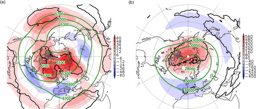
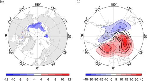
Winter atmospheric conditions in the Arctic and in surrounding regions have changed significantly between both periods. Tropospheric geopotential heights in the December to February season are displayed in Fig. 1a for 500 hPa. The difference plot for low minus high sea ice concentrations in preceding September shows a clear tendency to a negative NAO pattern. Positive height anomalies are visible in the Arctic in contrast to more negative anomalies in the mid latitudes. With a positive anomaly in the Aleutian low region the pattern does not resemble a typical negative AO situation. We performed an EOF analysis of geopotential heights and identified the first EOF in 500 hPa as the AO pattern. In the high ice period the average value of the associated PC was 0.02. In the low ice period it slightly decreased to an average value of −0.05. Both values are very low and do not differ significantly, therefore the reduced negative geopotential height gradient towards the North Pole in the troposphere does not entirely concur with AO changes. Our analysis identifies a continuation of the geopotential heights difference pattern into the stratosphere, which is barotropic in the Atlantic/European sector. Fig. 1b presents geopotential height anomalies for the low-high ice period in 10 hPa. The finding is similar to the tropospheric pattern with a strong positive geopotential height anomaly in the Arctic and weaker negative anomalies in the mid-latitudes. Again the climatological mean pattern, a negative gradient between mid-latitudes and the Arctic, is weakened by anomalies associated to the low ice period. This is linked to a weaker stratospheric polar vortex. The first EOF pattern for 10 hPa resembles these anomalies with an average value for the PC of 0.12 for the high ice phase and −0.20 for the low ice phase.

Fig. 1 ERA-Interim geopotential height differences (gpm) between low (2001–2012) and high (1980–2000) ice period for winter (DJF) in (a) 500 hPa and (b) 10 hPa. Green contours show the climatological mean (1980–2012), black contours the 90% confidence level calculated from a U test.

From 1980 to 1989 nine SSWs occurred while from 1990 to 1999 only two were detected. This difference in stratospheric conditions is documented by Charlton and Polvani (2007). Furthermore, the averaged PC of the first EOF for the 1990–1999 period suggests a higher tropospheric AO index of 0.10 compared to −0.13 for the 1980–1989 decade. In the stratosphere at 10 hPa the averaged PC values of the first EOF range from 0.16 for the 1990s and −0.08 for the 1980s. We therefore split the high ice period into two separate time periods from 1980 to 1989 and from 1990 to 1999 for further analysis. Figure 2a and 2b show the differences between these two periods at 500 and 10 hPa, respectively. The 1980s show increased 500 hPa geopotential heights in northern Siberia, Alaska and the American west coast, and around Greenland and the North Atlantic. Negative anomalies are found over Europe in the area from the East Asia to the central Pacific and at the American east coast. The pattern enhances the climatological stationary wave pattern shown in green contours and is in general agreement with a more negative AO phase in the 1980s. The difference pattern between the 1980s and the 1990s in the stratosphere at 10 hPa shows a dipole with a negative anomaly above north-western Canada and a positive anomaly with its maximum above the western part of Siberia, where the climatological minimum geopotential heights are located. This pattern leads to a filling of the geopotential heights minimum and a shift towards the Beaufort Sea in the 1980s. The displacement is confirmed by the climatological mean pattern with removed zonal mean, which shows an inversed dipole. The positive anomaly further extends over large parts of the mid-latitudes. Therefore, the poleward negative geopotential heights gradient is reduced especially in most parts of the mid-latitudes if the 1980s are compared to the 1990s. The overall finding is consistent with a weaker stratospheric polar vortex in the 1980s.

Fig. 2 ERA-Interim geopotential height differences (gpm) in (a, c, e) 500 hPa and (b, d, f) 10 hPa (a, b) between the 1980–1989 decade and the 1990–1999 decade, (c, d) between low ice period (2001–2012) and the 1980–1989 decade and (e, f) between low ice period (2001–2012) and the 1990–1999 decade for winter (DJF). Green contours show the climatological departures from the zonal mean (1980–2012), black contours the 90% confidence level calculated from a U test.

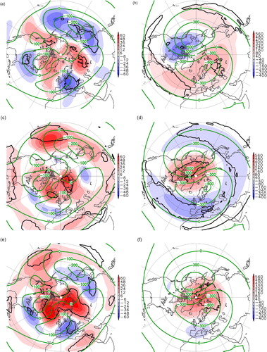
Figure 2c–2f show separate geopotential height differences between the low ice period 2001–2012 and the reference periods 1980–1989 and 1990–1999. In the troposphere the differences are stronger and more significant if compared to the 1990s as shown in Fig. 2e. This is in agreement to the difference in terms of the AO index and thus the pattern is very similar to the anomalies in Fig. 2a. But the positive anomaly in the Arctic Ocean and negative anomalies in the mid-latitudes persist even if compared to a more negative tropospheric AO situation during the 1980s as shown in Fig. 2c. A positive 500 hPa geopotential height anomaly is visible in Fig. 2c and 2e in the Aleutian Low region. The Aleutian Low is linked to the Pacific North America teleconnection pattern (PNA) and thus shows tropical influences. In the 1990s the PNA was in a more negative phase, related to higher than average pressure at the Aleutian Low, whereas the 1980s had a more positive PNA influence related to a lower than average Aleutian Low. Although the PNA modifies the Aleutian low between the 1980s and 1990s it could not explain the overall positive anomaly in the Aleutian Low region in the low ice period. A large fraction of the tropospheric differences between the three periods can be directly attributed to the variability of atmospheric teleconnection patterns. In the last decade a negative tropospheric NAO/AO-like anomaly pattern and a higher than average Aleutian Low persists, which suggests an influence by Arctic sea ice changes.

In the stratosphere the difference pattern between the low ice period and the 1980s in Fig. 2b as well as the difference pattern between the low ice period and the 1990s show a weakened polar vortex. This is in agreement with our EOF analysis, which suggests the most negative averaged PC value of the first EOF in the low ice phase. In the low ice period we find lower geopotential heights in Arctic regions as displayed in Fig. 1b. In Fig. 2d and 2f the general pattern describing a weaker polar vortex is still visible, but specific characteristics of the 1980s and 1990s play a role. The maximum positive difference is shifted to the Beaufort Sea in the 1980s (Fig. 2d). This is in agreement with the dipole pattern in Fig. 2b and the described shift of minimum geopotential heights to that area in the 1980s. Furthermore we find negative anomalies in the mid-latitudes in agreement with the reduced extent of the 1980s negative poleward geopotential height gradient to the mid-latitudes. In the 1990s the position and extent of the poleward negative geopotential height gradient is more comparable to the low ice phase.

In summary, we find a signal in the low ice period that is similar to a negative tropospheric NAO/AO anomaly and a reduced polar vortex in the stratosphere. In the troposphere this signal can only partly be explained by the first EOF since a strong positive anomaly in the Aleutian Low region during low ice conditions exists. This anomaly is neither covered by the AO nor by the PNA. In the stratosphere low sea ice conditions are connected with a weakened polar vortex.

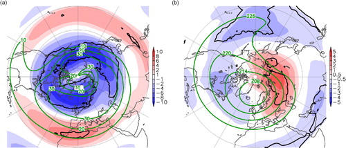
The strength of the stratospheric polar vortex is directly linked to the zonal wind fields in the stratosphere. The climatological mean zonal wind in 10 hPa in Fig. 3a shows the vortex, which is characterised by strong westerlies. The difference pattern between low and high ice phase shows a strong negative anomaly corresponding to a weaker polar vortex during the low ice period. This is in agreement with the geopotential height anomalies in Fig. 1b, which represent a reduced meridional pressure gradient. Reduced zonal winds together with increased EP fluxes by planetary waves, shown in Fig. 6, lead to an enhanced large-scale wave mixing. The stratospheric overturning circulation is strengthened due to enhanced planetary wave activity. Enhanced mixing and adiabatic warming over the Arctic leads to higher stratospheric temperatures over Siberia displayed in Fig. 3b. Both findings are in agreement with the observed changes in the geopotential heights and the negative AO phase in the troposphere.

Fig. 3 ERA-Interim (a) zonal wind (m/s) and (b) temperature differences (K) between low (2001–2012) and high (1980–2000) ice period for winter (DJF) in 10 hPa. Green contours show the climatological mean (1980–2012), black contours the 90% confidence level calculated from an U test.

For a more detailed examination of the influence of August/September low sea ice anomalies on the overlying atmosphere in the following winter we performed MCAs throughout the whole troposphere and stratosphere using sea ice concentration as the first variable and geopotential heights as the second variable. The patterns are shown as heterogeneous regression maps for the sea ice concentration and as homogeneous regression maps for the geopotential heights. The results for 500 hPa geopotential height are displayed in Fig. 4a–4d and for 10 hPa in Fig. 4e–4h. The first coupled pattern in Fig. 4a and 4b explains 55% of covariance and resembles the connection between the trend of decreasing late summer Arctic sea ice concentration and the negative NAO/AO signal in the troposphere at 500 hPa with a positive geopotential height anomaly over the Arctic Ocean that is opposite to the climatological mean pattern. Additionally, a positive anomaly in the North Pacific region is also present. Together with the negative anomaly over East Asia it shifts the climatological mean lower geopotential heights above the western Pacific more towards Asia and weakens the Aleutian low. The pair of patterns in Fig. 4e and 4f explains 61% of covariance between August/September sea ice concentration and winter geopotential heights in 10 hPa. The pattern of decreasing sea ice in Fig. 4e is connected to a reduced stratospheric polar vortex and a slight shift compared to the climatology as displayed in Fig. 4f. The associated time series of the sea ice concentration patterns for the first MCA in both heights are correlated with a coefficient above 0.9. Furthermore, all associated time series of adjacent geopotential height fields of the first MCA pattern are correlated with coefficients above 0.9 showing the continuous connection between the signal in the troposphere and the stratosphere.

Fig. 4 First (a, b and e, f) and second pair (c, d and g, h) of coupled patterns obtained by the Maximum-Covariance-Analysis (MCA) of August/September HadISST1 sea ice concentration (1979–2011) and ERA-Interim winter (DJF) geopotential height fields (1980–2012). Upper row displays the sea ice concentration anomaly maps in percent as heterogeneous regression maps. Lower row contains the corresponding anomaly maps for geopotential heights in 500 hPa (b, d) and 10 hPa (f, h) in gpm, shown as homogeneous regression maps. Black contours in (b) and (f) show the climatological mean (1980–2012) with 5100 gpm, 5200 gpm, and 5300 gpm isolines in (b) and 29000 gpm, 30000 gpm, and 30500 gpm isolines in (f) starting from the pole. Black contours in (d) and (h) show the climatological departures from the zonal mean (1980–2012) with 50 gpm contour interval in (d) and 150 gpm contour interval in (h). Negative contours are dashed.

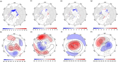
The second pair of MCA patterns in Fig. 4c and 4d explains 15% of covariance between August/September sea ice concentration and winter 500 hPa geopotential heights. The according pair of patterns for 10 hPa geopotential heights is displayed in Fig. 4g and 4h explaining 18% of covariance. Both sea ice concentration patterns in Fig. 4c and 4g again look very similar with a strong negative anomaly above the East Siberian Sea. Their associated time series are correlated (r=0.78). The coupled geopotential height pattern in 500 hPa in Fig. 4d exhibits a large positive anomaly over the North Pacific Ocean. This could be connected to the wave train changes described in Jaiser et al. (2012) and resembles the anomaly seen in the Aleutian height region before. The associated time series further reveals a negative correlation with the PNA (r=−0.69). In the Atlantic region the pattern corresponds to the climatological mean differences from the zonal mean with NAO-like anomalies. The stratospheric pattern in Fig. 4h exhibits a dipole with a positive anomaly over Canada and a negative anomaly over Siberia. Notably this is an eastward shifted strengthening of the climatological departures from the zonal mean and thus a strengthening of the quasi-stationary wave pattern. The shift between the tropospheric and stratospheric pattern occurs at the tropopause. Analysing these levels in more detail with a multiple correlation we can show that the tropospheric pattern is connected to the stratospheric pattern with coefficients larger than 0.9. In summary, our analysis of the second MCA patterns reveals a connection between a positive tropospheric geopotential height anomaly in the Pacific region and an eastward shifted wavenumber 1 pattern in the stratosphere.

A further MCA was performed to analyse the relation between winter meridional heat fluxes on planetary scales (10–90 d) and late summer sea ice. The results are shown in Fig. 5 for meridional heat fluxes at 10 hPa. A negative sea ice anomaly covering most of the Siberian seas covaries with an enhanced planetary scale heat flux pattern. The positive heat flux anomaly is placed over the western Siberian region extending to the North Atlantic with a secondary maximum and is linked to higher stratospheric temperatures in Fig. 3b. A negative anomaly is located over eastern Siberia and extents to the Canadian archipelago. The pattern explains 36% of covariance between August/September sea ice and meridional heat flux in 10 hPa during winter. The positive anomalies as well as the Canadian part of the negative anomaly amplify the climatological mean pattern shown as a black contour in Fig. 5b. The negative anomaly over eastern Siberia indicates a westward shift of the climatological pattern and overall weaker planetary scale meridional heat fluxes over the Pacific region. The North America-Pacific negative anomalies and Eurasian-Atlantic positive anomalies resembles a wave-1 pattern. Compared to the climatology reduced sea ice conditions are linked to enhanced stratospheric planetary scale heat fluxes over the North Atlantic-Eurasian region.

Fig. 5 First pair of coupled patterns obtained by the maximum covariance analysis of (a) August/September HadSST1 sea ice concentration (1979–2011) in percent displayed as heterogeneous regression map and (b) ERA-Interim winter (DJF) meridional heat flux on planetary scales (10–90 d) in 10 hPa (1980–2012) in Km/s displayed as homogeneous regression map. Black contour in (b) shows the climatological mean (1980–2012) with 20 Km/s contour interval. Negative isolines are dashed.

It is still not clear how SSWs and planetary scale heat flux anomalies are related. In the beginning of the low ice phase the frequency of SSWs regained the high level of the 1980s (Charlton and Polvani, 2007). Our analysis of stratospheric temperatures suggests SSWs in each year throughout the whole low ice phase. Within this period two major SSWs occurred in January 2009 and 2010 with record values in planetary wave activity (Ayarzagüena et al., 2011). Planetary scale meridional heat flux anomalies displayed in Fig. 5b could be directly connected to the warm anomalies during SSWs.

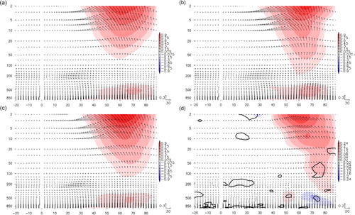
The coupling between tropospheric changes following to sea ice retreat and the overlying stratosphere is expected to be accomplished by upward propagating planetary waves. To investigate this we analyse the vertical component of the localised EP flux for the 10–90 d time-scale. We analyse the 1980s, the 1990s and the low ice period separately. The shading in Fig. 6a–6c indicates a weak connection between troposphere and stratosphere through upward propagating planetary waves in the 1980s in Fig. 6a. In the 1990s (Fig. 6b) EP fluxes between 200 and 100 hPa are enhanced with an anomalous strong upward component between 50 and 70°N. In the higher stratosphere between 70 and 90°N the upward EP flux is anomalous weak. The low ice period is also characterised by enhanced upward planetary wave propagation especially between 70 and 90°N (Fig. 6d). These anomalies lead to upward propagating waves north from 80°N around the tropopause, which can only be found in the low ice period (Fig. 6c). The stratospheric planetary scale EP flux activity is enhanced and shifted northward during low ice conditions. These upward propagating planetary waves interfere with the polar vortex and reduce its strength as diagnosed in the previous discussion. It is worth noting that these large differences originating from Arctic regions only occur in the low ice period. This indicates an influence of Arctic sea ice changes through changes in the diabactic heating triggered by higher Arctic temperatures.

Fig. 6 Zonal mean ERA-Interim vertical component of EP flux (m²/s², shaded) and vertical and meridional component (vectors) on planetary scales (10–90 d) for (a) the 1980–1989 decade (b) the 1990–1999 decade, (c) the low ice period (2001–2012) and (d) as differences between low (2001–2012) and high (1980–2000) ice phase for December. Black contours show the 90% confidence level calculated from a U test.

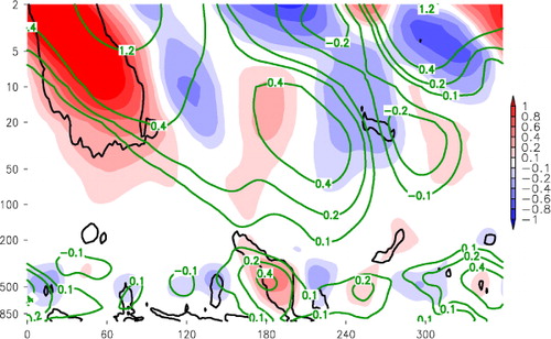
The key region of these zonal mean differences in the stratosphere is placed between 0 and 100°E (Fig. 7). The longitude dependent climatological pattern is enhanced by these anomalies, which is also in agreement with a more disturbed polar vortex due to an enhanced planetary wave pattern. The EP flux directly interacts with the zonal wind through its divergence. A negative forcing of the zonal wind in the region of maximal upward EP flux differences in the stratosphere (not shown) indicates a weakening of the polar vortex due to planetary wave interactions. This conclusion is in agreement with Garfinkel et al. (2010), who found positive wave-2 upward EP fluxes in connection with positive geopotential height anomalies around 60°N and 40°E in 500 hPa, similar to our results in Fig. 5b. In the troposphere the upward EP flux vanishes at about 300 hPa in Fig. 7. Enhanced upward EP flux that expand into this region and above can only be found in Pacific regions at 180°E and weaker at 90°W (Fig. 7). The strongest upward planetary wave propagation from the troposphere into the stratosphere occurs over the Pacific according to Plumb (1985). The anomaly is closely situated in the region of the EP flux divergence wave train like anomaly on planetary scales described by Jaiser et al. (2012) and might be further connected to the positive geopotential height anomaly we found in Fig. 1a and 4b in the Aleutian Low region. Additionally, Nishii et al. (2010) concluded that stratospheric planetary wave anomalies are the result of three-dimensional planetary wave propagation induced by tropospheric teleconnection patterns, e.g. the Western Pacific Pattern.

Fig. 7 ERA-Interim vertical component of EP flux vector differences (m²/s²) on planetary scales (10–90 d) between low (2001–2012) and high (1980–2000) ice period for December meridional mean cross-section between 66 and 80°N. Green contours show the climatological mean (1980–2012), black contours show the 90% confidence level calculated from a U test.

4. Conclusion

Reduced Arctic sea ice cover in August/September influences tropospheric and stratospheric circulations in the following winter. We showed that observed large-scale atmospheric changes as the negative tropospheric NAO/AO-like signal in winter extend barotropically into the stratosphere. During low ice conditions the stratospheric polar vortex is weakened and stratospheric polar temperatures are higher. The link between tropospheric and stratospheric processes is maintained through enhanced upward EP fluxes on planetary scales under low ice conditions. The low ice period is characterised by enhanced upward planetary wave propagation especially between 70 and 90°N. Positive tropospheric EP flux anomalies are found over Pacific and North American regions, which might be connected through three-dimensional wave propagation with positive anomalies in the middle stratosphere above the North Atlantic. A connection between meridional stratospheric heat fluxes on planetary scales (10–90 d) and late summer sea ice conditions was described. A negative sea ice anomaly covering most of the Siberian seas covaries with an enhanced planetary scale heat flux pattern in the stratosphere at 10 hPa. The positive stratospheric heat flux anomaly over the western Siberian region extending to the North Atlantic is linked to higher stratospheric temperatures and amplifies the climatological planetary-scale wave-1 pattern. The additional wave energy generated through synoptic and planetary wave interactions as described in Jaiser et al. (2012) is able to interact with the stratospheric polar vortex leading to the observed lower stratospheric polar vortex strength in the last decade.

To improve our understanding global atmospheric model experiments with prescribed sea ice conditions and well resolved stratospheric processes are needed. It is important to find out how the different mechanisms interact, which feedback loops are involved and how they impact on the large-scale circulation. This implies that these models need to reproduce the large-scale circulation and its low frequency variability properly, where deficits exist (Handorf and Dethloff, 2012). A resulting robust description of the influence of changes in surface conditions like sea ice and snow cover on the large-scale circulation in the troposphere and stratosphere could add distinct improvements to seasonal forecasting systems.

5. Acknowledgements

We wish to thank two anonymous reviewers for their beneficial comments and assistance.

References

- Ayarzagüena B , Langematz U , Serrano E . Tropospheric forcing of the stratosphere: a comparative study of the two major stratospheric warmings in 2009 and 2010. J. Geophys. Res. 2011; 116: D18114.
- Bader J , Mesquita M. D. S , Hodges K. I , Keenlyside N , Østerhus S , co-authors . A review on Northern Hemisphere sea-ice, storminess and the North Atlantic Oscillation: observations and projected changes. Atm. Res. 2011; 101: 809–834.
- Bell C. J , Gray L. J , Charlton-Perez A. J , Joshi M. M . Stratospheric communication of El Niño teleconnections to European winter. J. Climate. 2009; 22: 4083–4096.
- Blackmon M. L , Lau N.-C . Regional characteristics of the Northern Hemisphere wintertime circulation: a comparison of the simulation of a GFDL general circulation model with observations. J. Atmos. Sci. 1980; 37: 497–514.
- Blüthgen J , Gerdes R , Werner M . Atmospheric response to the extreme Arctic sea ice conditions in 2007. Geophys. Res. Lett. 2012; 39: L02707.
- Charlton A. J , Polvani L. M . A new look at stratospheric sudden warmings. Part I: climatology and modeling benchmarks. J. Climate. 2007; 20: 449–469.
- Cohen J , Barlow M , Kushner P. J , Saito K . Stratosphere–troposphere coupling and links with Eurasian land surface variability. J. Climate. 2007; 20: 5335–5343.
- Cohen J. L , Furtado J. C , Barlow M. A , Alexeev V. A , Cherry J. E . Arctic warming, increasing snow cover and widespread boreal winter cooling. Environ. Res. Lett. 2012; 7: 014007.
- Cohen J , Jones J . A new index for more accurate winter predictions. Geophys. Res. Let. 2011; 38: L21701.
- Czaja A , Frankignoul C . Observed impact of Atlantic SST anomalies on the North Atlantic Oscillation. J. Climate. 2002; 15: 606–623.
- Dee D. P , Uppala S . Variational bias correction of satellite radiance data in the ERA-Interim reanalysis. Q.J.R. Meteorol. Soc. 2009; 135: 1830–1841.
- Francis J. A , Vavrus S. J . Evidence linking Arctic amplification to extreme weather in mid-latitudes. Geophys. Res. Lett. 2012; 39: L06801.
- Garfinkel C. I , Hartmann D. L , Sassi F . Tropospheric precursors of anomalous Northern Hemisphere stratospheric polar vortices. J. Climate. 2010; 23: 3282–3299.
- Graf H.-F , Zanchettin D . Central Pacific El Niño, the “subtropical bridge,” and Eurasian climate. J. Geophys. Res. 2012; 117: D01102.
- Handorf D , Dethloff K . How well do state-of-the-art atmosphere-ocean general circulation models reproduce atmospheric teleconnection patterns?. Tellus A. 2012; 64: 19777.
- Hannachi A , Jolliffe I. T , Stephenson D. B . Empirical orthogonal functions and related techniques in atmospheric science: a review. Int. J. Climatol. 2007; 27: 1119–1152.
- Ineson S , Scaife A. A . The role of the stratosphere in the European climate response to El Niño. Nature Geosci. 2009; 2: 32–36.
- Inoue J , Hori M. E , Takaya K . The role of Barents sea ice in the wintertime cyclone track and emergence of a warm-Arctic cold-Siberian anomaly. J. Climate. 2012; 25: 2561–2568.
- Jaiser R , Dethloff K , Handorf D , Rinke A , Cohen J . Impact of sea ice cover changes on the Northern Hemisphere atmospheric winter circulation. Tellus A. 2012; 64: 11595.
- Kolstad E. W , Breiteig T , Scaife A. A . The association between stratospheric weak polar vortex events and cold air outbreaks in the Northern Hemisphere. Q.J.R. Meteorol. Soc. 2010; 136: 886–893.
- Liu J , Curry J. A , Wang H , Song M , Horton R. M . Impact of declining Arctic sea ice on winter snowfall. PNAS. 2012; 109: 4074–4079.
- Nishii K , Nakamura H , Orsolini Y. J . Cooling of the wintertime Arctic stratosphere induced by the western Pacific teleconnection pattern. Geophys. Res. Lett. 2010; 37: L13805.
- Orsolini Y. J , Senan R , Benestad R. E , Melsom A . Autumn atmospheric response to the 2007 low Arctic sea ice extent in coupled ocean–atmosphere hindcasts. Clim. Dyn. 2011; 38: 2437–2448.
- Overland J. E , Wood K. R , Wang M . Warm Arctic - cold continents: climate impacts of the newly open Arctic sea. Polar Research. 2012; 30: 15787.
- Petoukhov V , Semenov V. A . A link between reduced Barents-Kara sea ice and cold winter extremes over northern continents. J. Geophys. Res. 2010; 115: D21111.
- Plumb R. A . On the three-dimensional propagation of stationary waves. J. Atmos. Sci. 1985; 42: 217–229.
- Porter D. F , Cassano J. J , Serreze M. C . Local and large-scale atmospheric responses to reduced Arctic sea ice and ocean warming in the WRF model. J. Geophys. Res. 2012; 117: D11115.
- Preisendorfer R . Principal Component Analysis in Meteorology and Oceanography. Developments in Atmospheric Science.
- Rayner N. A , Parker D. E , Horton E. B , Folland C. K , Alexander L. V , co-authors . Global analyses of sea surface temperature, sea ice, and night marine air temperature since the late nineteenth century. J. Geophys. Res. 2003; 108: 4407. 10.1029/2002JD002670.
- Screen J. A , Deser C , Simmonds I . Local and remote controls on observed Arctic warming. Geophys. Res. Lett. 2012; 39: L10709. 10.1029/2012GL051598.
- Stroeve J. C , Serreze M. C , Barrett A , Kindig D. N . Attribution of recent changes in autumn cyclone associated precipitation in the Arctic. Tellus A. 2011; 63: 653–663. 10.1111/j.1600-0870.2011.00515.x.
- Trenberth K. E . An assessment of the impact of transient eddies on the zonal flow during a blocking episode using localised Eliassen-Palm flux diagnostics. J. Atmos. Sci. 1986; 43: 2070–2087.
- Von Storch H , Zwiers F. W . Statistical Analysis in Climate Research.
- Wu B. Y , Su J. Z , Zhang R. H . Effects of autumnwinter Arctic sea ice on winter Siberian High. Chinese Sci. Bull. 2011; 56: 3220–3228. 10.1007/s11434-011-4696-4.