Development of an idealised downstream cyclone: Eulerian and Lagrangian perspective on the kinetic energy

ABSTRACT

In this idealised modelling study, the development of a downstream cyclone, which closely follows the life-cycle of a Shapiro-Keyser cyclone, is addressed from a quasi-geostrophic kinetic energy perspective. To this end a simulation of a dry, highly idealised, dispersive baroclinic wave, developing a primary and a downstream cyclone, is performed. Kinetic energy and processes contributing to its tendency – in particular baroclinic conversion and ageostrophic geopotential fluxes – are investigated in three dimensions both in an Eulerian and a Lagrangian framework from the genesis of the downstream cyclone as an upper-level kinetic energy centre, over frontal fracture to the fully developed cyclone showing the characteristic T-bone surface frontal structure, with a strong low-level jet along the bent-back front. Initially the downstream cyclone grows by the convergence of ageostrophic geopotential fluxes from the primary cyclone, but as vertical motions intensify this process is replaced by baroclinic conversion in the warm sector. We show that kinetic energy released in the warm sector is radiated away at all levels by ageostrophic geopotential fluxes: in the upper troposphere they are directed downstream, while in the lower troposphere they radiate kinetic energy to the rear of the cyclone. Thereby, vertical ageostrophic geopotential fluxes, their location and divergence, are identified to play a major role in the intensification of the cyclone in the lower troposphere and for the formation of the low-level jet. Low-level rearward ageostrophic geopotential fluxes converging along the bent-back front are shown to be a general characteristic of an eastward propagating baroclinic wave.

• idealised extratropical cyclone
• local energetics
• downstream development
• low-level jet
• baroclinic wave
• energy dispersion
• three-dimensional ageostrophic geopotential fluxes

1. Introduction

Margules (1905) penned a remarkable essay on the energetics of storms, in which the atmosphere's potential energy was identified as storms’ major source of kinetic energy. Margules states,1 ‘The source of a storm, as far as I can tell, can only be found in the potential energy’ and furthermore ‘the storm is therefore generated due to ascending and descending air …’. He concentrated on what he called the generation of available kinetic energy from the total potential energy of the system. He realised that by adiabatically redistributing two air masses with different densities in such a way that the storm's centre of mass is lowered, the storm gains kinetic energy. Today this process is known as baroclinic conversion from available potential energy (APE) to kinetic energy (KE). The APE was formally introduced by Lorenz (1955) in his work on the maintenance of the general circulation. Analysis of APE and KE budgets on a global scale developed into a discrete branch of atmospheric research (Oort, 1964; Oort and Peixóto, 1974) and has become a widely used diagnostic tool in today's climate research (e.g. O'Gorman and Schneider, 2008). Energy budget analysis of individual storms and wave packets became feasible with increasing data resolution (e.g. Orlanski and Katzfey, 1991). On the scale of extratropical cyclones, the quasi-geostrophic (QG) theory provides a convenient framework to study the governing dynamical mechanisms during the life-cycle of a system. The QG KE tendency equation in height coordinates, which we will derive in Section 2, is given by1

where , v_G denotes the two-dimensional geostrophic wind and u _a is the three-dimensional ageostrophic wind, defined as (Pedlosky, 1987). Throughout the article, three-dimensional wind vectors will be denoted by the letter u and two-dimensional ones by the letter v. The perturbation pressure p*(x,y,z,t) is the deviation from the reference pressure p ₀(z), which itself is in hydrostatic balance with the reference density ρ ₀(z). Along the geostrophic flow, the KE changes according to the divergence of the ageostrophic geopotential fluxes2 . (I, in eq. 1) and baroclinic conversion (II) from APE into KE. The ageostrophic geopotential fluxes account for the dispersion of KE (Orlanski and Katzfey, 1991) by removing KE in places where the fluxes are divergent and depositing it again in areas where they converge.

This local perspective on the energetics has been strongly fostered by a series of publications by Orlanski (Orlanski and Katzfey, 1991; Orlanski and Chang, 1993; Orlanski and Sheldon, 1993), culminating in a conclusive paper in which the paradigm of (up- and) downstream development of baroclinic waves by ageostrophic geopotential fluxes was introduced (Orlanski and Sheldon, 1995). Its main idea is that downstream disturbances are initiated by the convergence of ageostrophic geopotential fluxes at upper levels before the onset of baroclinic conversion. The geopotential fluxes thereby draw KE from an upstream disturbance and initiate the latter's decay. As recently as the downstream disturbance has been established, baroclinic conversion sets in and takes over its growth process. Subsequently, the growth of the disturbance is counteracted again by downstream radiation of KE via ageostrophic geopotential fluxes. As Orlanski and Sheldon (1995) demonstrated, upper- and low-level ageostrophic geopotential fluxes differ in a fundamental aspect: in the upper troposphere they are directed downstream, while in the lower troposphere they point upstream. Downstream dispersion of KE and especially the timing of its onset with respect to a cyclone's life-cycle influences its decay to a considerable extent, which was demonstrated in a study of explosively deepening cyclones over North America, which were characterised by different decay characteristics (Decker and Martin, 2005). Lackmann et al. (1999) applied the local energy perspective to the intensification of jet streaks during the field campaign ERICA. By analysing the evolution of eddy kinetic energy at different levels, they pointed out that an upper-level KE centre is established prior to the growth of a KE centre in the lower troposphere.

The aim of this study is to investigate in depth the three-dimensional evolution of KE and its redistribution by advection and ageostrophic geopotential fluxes within a single, highly idealised cyclone. The cyclone's life-cycle is traced from its upper-level initiation until the development of a low-level jet. We demonstrate that ageostrophic geopotential fluxes do not only play a major role in the dispersion of the baroclinic wave's KE, but also in the redistribution of KE within the cyclone in the lower troposphere. In particular, we provide evidence that their convergence is essential for the formation of a low-level jet along the bent-back extension of the warm front, which in the following we will refer to as the bent-back front. Such low-level jets do not only bring potentially damaging winds (Grønås, 1995), but over the ocean they also induce significant fluxes of sensible and latent heat (Boutle et al., 2010). The KE analysis is performed both from an Eulerian and a Lagrangian perspective. The Eulerian perspective allows us to study local tendencies of KE and to relate them to individual structures of the cyclone such as the upper-tropospheric trough and the low-level frontal zones. In order to assess the relative importance of baroclinic conversion and the convergence of ageostrophic geopotential fluxes for the tendency of KE along the flow, we supplement the Eulerian analysis by a trajectory analysis, which hides the advective tendencies from the actual physical forcings experienced by the air parcels.

We begin with a recapitulation of the KE equation and its derivation and introduce the reader to the numerical set up of the simulation (Section 2). The overall synoptic evolution of the considered cyclone is described in Section 3. The main part of this article (Section 4) contains the assessment of the energetics.

2. Methodology

2.1. QG KE equation

The KE diagnostics is performed based on the QG KE equation. It is derived from the QG pseudo-momentum equation (Holton, 2004) by multiplication with ρ ₀ v _G 2

where the geostrophic wind is given by . The pressure advection term v_a ·∇ _h p* acts as the only source or sink of KE along the geostrophic flow. It thus includes the gain of KE by baroclinic conversion. By making use of the anelastic continuity equation , the second term on the left hand side of eq. (2) can be decomposed into the divergence of horizontal ageostrophic geopotential fluxes and an additional term,3

Manipulation of the second term on the right-hand side leads to the divergence of the vertical geopotential flux and the baroclinic conversion term4

which inserted into eq. (3), yields terms (I) and (II) of eq. (1)5

At this point, we emphasise that the geopotential flux vectors are only determined up to the addition of a non-divergent vectorfield. The chosen gauge of the flux vectors is particularly suited for the representation of the actual flux of geopotential (Orlanski and Katzfey, 1991) because the non-divergent geostrophic component has been removed from the overall geopotential flux vector p*u . By making use of the hydrostatic approximation, the baroclinic conversion term may be rewritten in a physically more intuitive form,6

Hence, baroclinic conversion increases KE when air warmer than its environment rises, or when colder air sinks. In Section 3, vertical averages of eq. (2) will be considered. To this end we define the vertical average of Φ(x,y,z,t) (e.g. KE) as7

where z _top denotes the height of the model domain.

2.2. Setup of the numerical simulation

For the purpose of this study, we consider a simulation identical to the dry run in Schemm et al. (2013). It is performed with an f-plane version of the non-hydrostatic weather prediction model COSMO (Steppeler et al., 2003) centred at 45°N. The integration domain encompasses a 16 800 km long periodic channel with a width of 8 400 km, reaching up to a height of 12 km. The grid is Cartesian with a horizontal spacing of approximately 21 km (0.18°) and 60 equidistant levels in the vertical with a spacing of 200 m. At the meridional boundaries, the fields are relaxed towards the initial state's boundary values. At the top, we enable Rayleigh damping, whereas the bottom is a flat surface with free-slip boundary conditions. We restrict the simulations to purely dry dynamics by switching off all parameterisations (microphysics, surface fluxes, turbulence, and radiation).

The initial state is composed of a zonally uniform, baroclinic jet in hydrostatic balance and a finite amplitude perturbation in the form of a positive upper-level potential vorticity (PV) anomaly (Wernli et al., 1999; Schemm et al., 2013). The background jet with a wind speed maximum of 40 m s⁻¹ is constructed following Olson and Colle (2007) with some minor modifications [see Schemm et al. (2013) for details]. The PV anomaly of the form8

has an amplitude of A=2-pvu (PV units3 ) and decay lengths of L _x =L _y =1000 km in the horizontal and L _z =4000 m in the vertical. Its centre is at a height of z _pos =8 km and its meridional position is in the middle of the channel, collocated with the axis of the basic state jet. The perturbation wind field is obtained from a QG PV inversion and is superposed on the background jet, which leads to peak perturbation winds with an amplitude of 10 m s⁻¹ in the vicinity of the jet maximum. A vertical section across the centre of the anomaly is shown in Fig. 1. Vertical reference profiles of p ₀, θ ₀ and ρ ₀, that are required for the KE diagnostics, are obtained by meridionally averaging these quantities of the unperturbed basic state.

Fig. 1.  Initial state: meridional cross-section at the position of the potential vorticity anomaly. Displayed are zonal wind (black contours, from 5 m s⁻¹ to 35 m s⁻¹), isentropes (gray, every 5 K) and the 2-pvu tropopause (green). Colors show the perturbation of the zonal wind by the initial potential vorticity anomaly in intervals of 2.5 m s⁻¹ with blue indicating easterly and red westerly winds.

Trajectories, along which QG KE and terms (I, II) of eq. (1) are traced, are calculated using the Lagrangian Analysis Tool LAGRANTO (Wernli and Davies, 1997).

3. Synoptic evolution

Before presenting the energetics of the downstream cyclone, in this section an overview is given of the synoptic evolution of the developing baroclinic wave with a focus on the downstream cyclone. A more extensive description can be found in Schemm et al. (2013).

3.1. Synoptic evolution: vertically averaged KE of the baroclinic wave

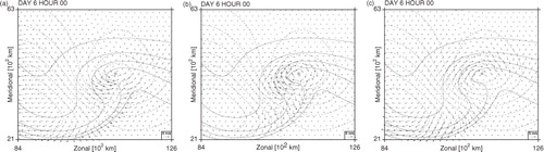
The evolution of the upper-level trough and ridge pattern is shown in Fig. 2 by the 2-pvu isoline on 320 K (green contour), while surface isentropes are used to depict the surface frontal development. The initial state upper-level jet goes along with a zonal band of high KE, which is perturbed by the cyclonic wind field induced by the PV anomaly. Consequently, the KE of the jet is enhanced south and reduced north of the anomaly, as can be seen from the vertically averaged KE (dashed contours) in Fig. 2a and 2b. By day 4 (Fig. 2c) the KE minimum north of the cyclone becomes encircled by high KE air. Downstream development becomes evident by the formation of a downstream KE centre at upper levels with a significant magnitude after day 4 and a fully developed downstream jet maximum two days later (Fig. 2d).

Fig. 2.  Time evolution of the baroclinic wave at day 0 (a), day 2 (b), day 4 (c) and day 6 (d). Shown are vertically averaged kinetic energy (dashed, contours for 100, 300, 500 and 700 J m⁻³) and pressure advection v _a ·∇ _h p* (color). The green contour indicates the 2-pvu isoline on 320 K and gray solid contours depict surface potential temperature (every 6 K).

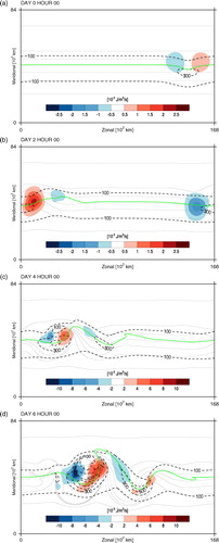
In Fig. 2 the vertically averaged pressure advection term v _a ·∇ _h p* is shown in colour. Blue indicates a tendency for an increase of KE along the geostrophic flow, whereas red indicates a decrease. At the location of the primary disturbance, we observe a dipole pattern with generation of KE in the entrance and reduction in the exit region of the KE centre. Advection of high (low) KE air by cyclonic geostrophic winds maintains the relative KE maximum (minimum) south (north) of the cyclone's core. The dipole pattern persists as the cyclone evolves. Thus, the pressure advection term counteracts the translation of the KE centre by advection. From day 2 onward a region with a tendency for increase can be identified downstream, just to the east of the weakened basic state jet. This promotes the formation of the developing downstream cyclone.

3.2. Synoptic evolution: downstream cyclone

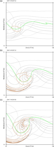
The downstream cyclone develops from top to bottom within a baroclinic zone by sinking motion below the upper-level jet. The incipient frontal fracture stage at day 5 hour 12 is depicted in Fig. 3a. The baroclinic zone differentiates into the cold and warm front and subsequent frontal development closely follows the life-cycle of a Shapiro-Keyser cyclone (Shapiro and Keyser, 1990). Warm air from the south is advected into the warm sector and is lifted as it hits upon the warm front. Aligned with the intense horizontal pressure gradient behind the developing cold front, just below the upper-level trough (2-pvu isoline on 320 K, green), a first maximum in low-level winds can be identified (brown contour). At this stage, the pressure minimum is collocated with the regions of strongest curvature of the surface isentropes. Until day 6 hour 12 the pressure minimum migrates south-westwards with respect to the surface fronts, while the cold front intensifies considerably (Fig. 3b). Below the deepening upper-level trough, surface winds increase along the incipient bent-back front, where pressure gradients are strongest. The cyclone then transitions from the frontal fracture to the T-bone stage and by day 7 an intense low-level north-westerly jet has formed with winds above 35 ms⁻¹ (dotted area, Fig. 3c).

Fig. 3.  Synoptic evolution of the downstream cyclone: incipient frontal cyclone (a), late frontal fracture (b), and T-bone stage (c). Surface potential temperature (black solid, every 4 K), surface pressure (dashed, every 10 hPa), surface wind speeds (brown, contours from 20 m s⁻¹ in steps of 5 m s⁻¹ with areas above 35 m s⁻¹ dotted) and 2-pvu isoline on 320 K (green).

In the following section, the energetics of the downstream cyclone will be investigated in detail, starting with the genesis of the cyclone in the lower troposphere below the upper-level jet maximum.

4. Energetics of the downstream cyclone

By day 4, a downstream upper-level jet streak (Fig. 4a) has been established and extends to the southernmost tip of the developing trough, indicated by the KE contours (dashed lines). The upper-level trough and ridge pattern is indicated by the 2-pvu isoline on 320 K (green contour), while grey lines depict isolines of potential temperature at the surface. The KE centre of the jet grows due to convergence of ageostrophic geopotential fluxes ∇·(p*u _a ) (shown in colours) in its entrance region, drawing KE from the primary cyclone's upper-level jet, which was also discussed in terms of energy budgets in Schemm et al. (2013). Interestingly already at this early stage ageostrophic geopotential fluxes radiate KE further downstream away from the jet exit region, albeit only weakly.

Fig. 4.  Initiation of the lower-tropospheric cyclone. Shown in (a) are upper-level divergence of ageostrophic geopotential fluxes ∇·(p*u _a ) (color) and kinetic energy (dashed, contrours for 100, 300 and 500 J m⁻³) at a height of 6 km as well as the 2-pvu isoline on 320 K (green). Potential temperature at the surface is shown by gray, solid lines (every 6 K). Panel (b) shows baroclinic conversion (color) at 2 km height and kinetic energy at the surface (dashed, contours for 100, 300 and 500 J m⁻³). Also shown are surface pressure (thin dashed, every 5 hPa) and potential temperature (gray solid, every 6 K). The location of strongest downward motion at a height of 2 km is indicated by the −0.0075 m s⁻¹ contour of the vertical wind (green).

4.1. Initiation of the lower-tropospheric cyclone

Within an elongated zone below the jet's KE maximum subsidence occurs due to the convergence of the ageostrophic wind above (not shown) in the region where the full wind changes from super- (around the ridge) to sub-gestrophic (around the downstream trough). At the same time in the lower troposphere, north-westerly winds advect cold air and establish a negative potential temperature anomaly below the trough. Consequently, wθ*>0 and the subsidence goes along with baroclinic generation of KE. This is illustrated in Fig. 4b, showing baroclinic conversion on 2 km and surface KE. At the tip of the area of baroclinic conversion a surface KE centre becomes evident. Note that the maximum of baroclinic generation in the lower troposphere is shifted north-westwards with respect to the region of most intense subsidence (green contour).

To assess the relative importance of baroclinic conversion and the convergence of ageostrophic geopotential fluxes for the development of the initial low-level KE centre, we consider trajectories ending at day 4 hour 12 in the low-level KE centre. From every grid point on the lowest three model levels (100–500 m) of the computational grid within a box enclosing the 100 J m⁻³ contour of KE, trajectories are started and calculated backward4 in time for 1.5 d based on hourly model output. Only those 4688 trajectories are considered that have a KE of at least 100 J m⁻³ at day 4 hour 12 (see schematic in upper left corner of Fig. 5a).

Fig. 5.  (a) Evolution of kinetic energy, (b) baroclinic conversion and (c) ageostrophic geopotential flux divergence along 1.5 d trajectories ending at day 4 hour 12 in the low-level KE center (KE ≥100 J m⁻³) and a height between 100 and 500 m. The target area on the lowest model level is schematically depicted in the upper left corner of (a). The trajectories are divided in two categories depending on whether the divergence of ageostrophic geopotential fluxes is positive (red) or negative (blue) at day 4 hour 12. The standard deviation (±σ) within each category is indicated by the shading. Note the different scales used in (b) and (c).

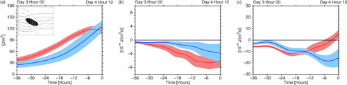
Figure 5 shows the evolution of KE, baroclinic conversion, and ageostrophic geopotential flux divergence along these trajectories, which are divided in two categories: trajectories ending in an area of ageostrophic geopotential flux convergence (blue, 3762 trajectories) and those ending in an area of divergence (red, 926 trajectories). Already before the trajectories start to descend, ageostrophic geopotential flux convergence leads to a steep rise of KE. Roughly after 12 hours the parcels descend modestly by 20–30 hPa (pressure evolution not shown), which additionally contributes to their increase of KE via baroclinic conversion. The magnitude of baroclinic conversion, however, remains below that of the ageostrophic geopotential flux convergence by a factor of three. Also because the convergence of ageostrophic geopotential fluxes sets in much earlier, its integrated contribution (roughly 110 J m⁻³ per trajectory) is seven to eight times larger than the increase of KE by baroclinic conversion (roughly 15 J m⁻³ per trajectory).5 Thus, in the early development of the downstream cyclone, ageostrophic geopotential flux convergence and subsequent advection is the primary mechanism by which the low-level KE centre grows. The mechanism responsible for the convergence of ageostrophic geopotential fluxes will be addressed below in Section 4.2.

Between day 3 hour 18 and day 4, the ageostrophic geopotential flux convergence starts to decline for certain air parcels and subsequently turns into divergence. Those parcels ending in a region of ageostrophic geopotential flux divergence are found at higher pressure values and thus are located on the anticyclonic side of the surface KE centre, while the others end at lower pressure and hence on the cyclonic side. Consequently, KE continues to increase for the parcels on the cyclonic side, while those on the anticyclonic side of the KE centre experience a decline of KE.

4.2. Redistribution of KE by the ageostrophic circulation

As found by the trajectory analysis, the low-level ageostrophic geopotential flux divergence reveals a dipole pattern with convergence to the north-east and divergence to the south-west of the surface KE centre, shown at day 5 in Fig. 6a. Overall the local increase of KE on the cyclonic side is more intense than the loss on the anticyclonic side of the KE centre. This has the important consequence that the KE maximum experiences an intensification due to ageostrophic geopotential fluxes on the cyclonic side.

Fig. 6.  Redistribution of kinetic energy due to the ageostrophic circulation. (a) shows the divergence of ageostrophic geopotential fluxes ∇·(p*u_a ) (color) at the surface and the −8 J m⁻² s⁻¹ isoline of vertical ageostrophic geopotential fluxes at 2 km (blue) at day 5. (b) shows the divergence of ageostrophic geopotential fluxes (color) and horizontal ageostrophic geopotential flux vectors with a magnitude greater than 3000 J m⁻² s⁻¹ at day 6. Also shown are surface fields of KE (dashed, contours for 100, 200, 300 and 400 J m⁻³), pressure (thin dashed, every 5 hPa) and potential temperature (solid gray, every 6 K). The cross-hatched symbol shows the location of the surface pressure minimum.

At day 6 (Fig. 6b) the surface baroclinic zone has fractured and the frontal pattern is reminiscent of the incipient T-bone stage, characterised by a rearward extension of the warm front. In addition to the discussed dipole pattern of the ageostrophic geopotential fluxes, we find weak divergence in the warm sector of the cyclone. Additional convergence occurs along the trailing cold front. The horizontal ageostrophic geopotential flux vectors p*v _a are directed away from the warm sector, pointing along the warm front and its incipient bent-back extension and finally converge in the rear of the cyclone. Similarly, ageostrophic geopotential flux vectors point away from the divergence south-west of the KE centre towards the trailing cold front.

How can the direction of the ageostrophic geopotential fluxes along the warm front, the pattern of weak divergence in the warm sector and the intense convergence along the bent-back warm front be understood? To answer this question we have to turn our attention to the low-level ageostrophic circulation and the vertical ageostrophic geopotential fluxes.

4.2.1. Low-level ageostrophic circulation.

The low-level horizontal ageostrophic geopotential flux vectors and their associated divergence pattern are a consequence of the low-level pressure anomalies p* propagating eastward and the ageostrophic circulation, which arises due to differential pressure tendencies and the curvature of the flow. Solving the QG pseudo-momentum equation for the horizontal ageostrophic wind, , and expressing the geostrophic wind in terms of p*, yields the decomposition of the horizontal ageostrophic wind into isallobaric and advective components (Holton, 2004).9

The isallobaric wind arises due to differential mass flow into or out of the air column above. Thus, it is opposed to the horizontal gradient of pressure tendency.

In the very idealised case of eastward propagating, circular pressure anomalies as shown in Fig. 7a, the isallobaric wind points from west to east in the negative anomaly and vice versa in the positive anomaly (red arrows). It is largest at locations where the gradient of pressure tendency is maximum, which is near the centre of the low and the high, respectively. The advective wind captures the effect of curvature and of vector length change of the geostrophic flow along itself. For cyclonic as well as anticyclonic geostrophic curvature its contribution is anticyclonic (yellow arrows). Combining isallobaric and advective ageostrophic winds, we find that they counteract each other to the south of the negative anomaly while they are parallel to the north (orange arrows).

Fig. 7.  Schematic of the horizontal ageostrophic circulation and ageostrophic geopotential fluxes associated with a circular, eastward propagating lower-tropospheric cyclone L and an anticyclone H. Depicted are (a) the low-level ageostrophic circulation and its decomposition into isallobaric and advective component and (b) horizontal ageostrophic geopotential fluxes and their divergence and convergence pattern.

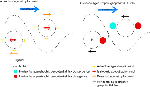
Taking the sign of the pressure anomalies into account the distribution of the ageostrophic wind yields a net upstream flux of energy by ageostrophic geopotential fluxes (black arrows in Fig. 7b). This is in line with the results of Orlanski and Sheldon (1995). However, since p* vanishes somewhere between the cyclone and the anticyclone, the p* =0 contour acts as a barrier for the low-level horizontal ageostrophic geopotential fluxes. Consequently the latter cannot point across the p*=0 contour and there has to be convergence of horizontal fluxes on the cyclonic and divergence on the anticyclonic side (blue and red dots). As can be inferred from the p*=0 contour a similar barrier exists in the warm sector of the downstream cyclone and the ageostrophic geopotential fluxes must diverge there. Therefore, there is no continuous upstream radiation of KE by ageostrophic geopotential fluxes at low levels from the cyclone to the anticyclone (and further to the upstream cyclone), but an upstream directed redistribution of KE within the cyclone (and the anticyclone) in the lower troposphere.

Figure 8 shows the ageostrophic wind and its decomposition into isallobaric and advective components at the surface at day 6. The isallobaric wind (Fig. 8a) is largest in the southern half of the low pressure system, which is due to enhanced gradients of pressure tendency across the cold front. Furthermore, the magnitude of the advective ageostrophic wind (Fig. 8b) varies along closed pressure contours encircling the low pressure system because of the non-circular distribution of KE, which is maximum to the west and to the north of the cyclone. Thus, isallobaric and advective winds cancel each other in the southern half of the cyclone, while in the north the advective wind is slightly enhanced by the isallobaric wind. For the anticyclone east-west oriented isallobaric winds arising from eastward propagation and increase of the shallow pressure maximum dominate, while cross frontal isallobaric winds play a minor role. Hence, the advective ageostrophic wind and the isallobaric wind are antiparallel to the north and parallel to the south of the anticyclone. This agrees well with the idealised arguments advanced above. Therefore, the observed horizontal ageostrophic geopotential fluxes are mainly a consequence of the ageostrophic circulation associated with eastward propagating pressure anomalies. However, horizontal fluxes alone are not able to explain the different magnitude of divergence on the anticyclonic and of convergence on the cyclonic side of the KE center, nor the weak divergence in the warm sector.

Fig. 8.  (a) Surface isallobaric and (b) advective wind contributions to (c) the total ageostrophic wind. Background fields are surface potential temperature (solid, every 6 K) and pressure (dashed, every 5 hPa).

4.2.2. Vertical ageostrophic geopotential fluxes.

In order to understand the much stronger convergence to the west of the cyclone center compared to the divergence in the warm sector, and the weak divergence on the anticyclonic side of the surface KE centre (see Fig. 6b) vertical ageostrophic geopotential fluxes need to be taken into account. Vertical ageostrophic geopotential fluxes are not equally distributed on the cyclonic and the anticyclonic side of the surface KE centre (Fig. 9). On the cyclonic side, where p*<0, the downward motion is associated with upward fluxes (wp*>0) and vice versa on the anticyclonic side (wp*<0). The most intense downward motion is found on the anticyclonic side (green contour in Fig. 4b). As a consequence the downward fluxes on the anticyclonic side reach up to 15 J m⁻² s⁻¹, whereas upward fluxes on the cyclonic side are below 2 J m⁻² s⁻¹, and thus are weaker by more than a factor of 7 (see Fig. 9). The downward fluxes converge near the surface and they are collocated with the divergence of the horizontal fluxes, which in consequence is efficiently reduced. This is supported by the −8 J m⁻² s⁻¹ contour (blue) in Fig. 6a. Now as KE grows primarily on the cyclonic side, so does the pressure gradient and thus the cyclone deepens at a faster rate than the anticyclone. In the warm sector the divergence of horizontal fluxes is counteracted by downward fluxes due to lifting of air parcels ahead of the cold front and over the warm front.

Fig. 9.  Same as Fig. 6a but for vertical ageostrophic geopotential fluxes at 2 km at day 5. Note the different scales for downward (blue) and upward (red) fluxes.

This remarkable interplay between horizontal and vertical fluxes on the cyclonic and anticyclonic side of the surface KE centre is a general feature of a growing baroclinic wave. During the growing phase of a baroclinic wave the pressure perturbation tilts backward (to the west) with height (e.g. Eady, 1949). This backward tilt ensures the different magnitude of the vertical ageostrophic geopotential fluxes on the cyclonic and the anticyclonic side of the KE centre.

4.3. The low-level jet

By day 6 hour 18 (Fig. 10), the cyclone shows the characteristic T-bone frontal structure with a strong bent-back front. Northerly winds reach up to 45 m s⁻¹ at its tail. In accordance with the thermal wind relation, this KE maximum decays with height and it extends only up to 700 hPa, as evidenced by the cross-section in Fig. 11a. The location of the cross-section is shown in Fig. 11b. At about 500 hPa, in the region of the northerly jet (J1), ageostrophic geopotential fluxes from the primary cyclone converge, while they diverge in the region of the southerly jet (J2) and radiate KE downstream. Therefore, the warm sector, where most of the baroclinic conversion of APE into KE takes place, is an area of overall ageostrophic geopotential flux divergence extending over the entire height of the troposphere.

Fig. 10.  Formation of the low-level jet at day 6 hour 18. Shown are divergence of ageostrophic geopotential fluxes ∇·(p*u _a ) (color), horizontal ageostrophic geopotential flux vectors p*v_a greater than 6000 J m⁻² s⁻¹, and kinetic energy (dashed, for 300, 600, 900 and 1200 J m⁻³) at the surface. Downward ageostrophic geopotential fluxes at a height of 2 km are indicated by the −20 J m⁻² s⁻¹ contour (blue) and upward fluxes by the 10 J m⁻² s⁻¹ contour (red). The background fields are surface pressure (thin dashed, every 10 hPa) and surface potential temperature (solid gray, every 6 K). The cross-hatched symbol shows the location of the surface pressure minimum.

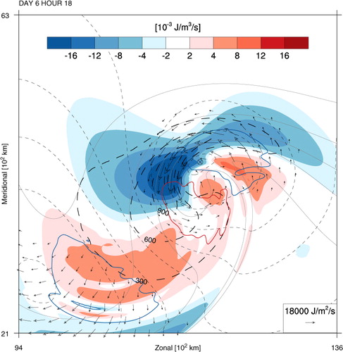
Downward fluxes due to rising air in the warm sector of the cyclone (p*<0) (see the –20 J m⁻² s⁻¹ contour (blue) in Fig. 10) feed KE into the lower troposphere. Accordingly in the warm sector the vertical ageostrophic geopotential fluxes radiate baroclinically generated KE from the mid and the upper troposphere to the lower troposphere, where they feed the KE directly into horizontal fluxes. As a consequence, the overall divergence at low levels in the warm sector is weak (Fig. 10).

Low-level advection of KE by the geostrophic flow (v _G ·∇ _h E _K ) is depicted in Fig. 11b. While ageostrophic geopotential fluxes redistribute KE between KE centres, advection redistributes KE within KE centres from their entrance to their exit (with respect to the flow direction). In particular the cyclonic flow advects KE along the bent-back front behind the cold front.

Fig. 11.  Panel (a) shows a section across the downstream cyclone in the T-bone stage at day 6 hour 18 with divergence of ageostrophic geopotential fluxes ∇·(p*u _a ) (color), kinetic energy (dashed, every 200 J m⁻³ from 300 J m⁻³) and potential temperature (gray solid, every 4 K). The location of the cross-section is shown in (b). J1 denotes the southward jet, J2 the northward jet, CF the cold front, WF the warm front and BF the bent-back front. Panel (b) is the same as Fig. 10 but with advection of kinetic energy v_G ·∇ _h E _K (color).

4.3.1 Lagrangian perspective.

In order to underpin that the air parcels forming the low-level jet gain their KE from ageostrophic geopotential flux convergence just before they arrive in the KE maximum, we consider 2 d trajectories ending at day 6 hour 18 at the tail of the bent-back front. The trajectory calculations are performed as in Section 4.1, except that the target area is delimited now by the 900 J m⁻³ contour of KE of the low-level jet and restricted to the lowest model level (100 m above ground). The endpoints of the 371 trajectories are shown in Fig. 12a.

Fig. 12.  (a) Evolution of kinetic energy, (b) baroclinic conversion and (c) divergence of ageostrophic geopotential fluxes along 2 d trajectories arriving at day 6 hour 18 in the low-level jet (KE ≥900 J m⁻³). Panel (a) shows the subset of trajectories located at the northern boundary of the 900 J m⁻³ contour of KE (dashed) at day 6 hour 18, and colors indicate KE at the midpoint of each line segment. Black dots denote the position of every trajectory at day 6 hour 18. Surface pressure (thin dashed, every 10 hPa) and potential temperature (solid, every 10 K) at day 6 hour 18. Note the different scales used in (b) and (c). The shading represents the standard deviation ±σ.

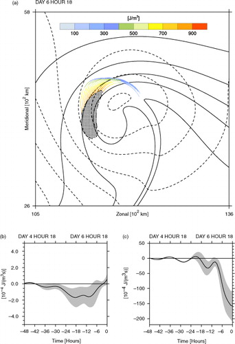
The trajectories move coherently along the warm front and have their origin in the south of the warm sector. Initially their KE is below 50 J m⁻³, corresponding to geostrophic winds of less than 10 m s⁻¹. In the warm sector of the cyclone, the KE increases only slightly through baroclinic conversion (Fig. 12b) and geopotential fluxes (Fig. 12c). Roughly 12 hours before their arrival in the jet maximum the KE of all parcels abruptly increases as the trajectories move towards the warm front, slope around the bent-back front and thereby enter the region of geopotential flux convergence. On day 6 hour 18 the average geostrophic wind of the air parcels is approximately 45 ms⁻¹. Compared to the averaged gain of KE by convergent ageostrophic geopotential fluxes (456 J m⁻³), baroclinic conversion along the trajectories is very weak (12 J m⁻³), yielding a total increase of KE by 468 J m⁻³. This reveals a discrepancy between the actual gain of KE (989 J m⁻³) and the increase of KE indicated by ageostrophic geopotential flux convergence and baroclinic conversion by 521 J m⁻³. For the most part this must be ascribed to the QG approximation, in particular to the overestimation of KE due to the fact that the actual wind is sub-geostrophic in the KE centre (see Section 5.1). Still the trajectory calculations clearly underpin the dominance of convergence of ageostrophic geopotential fluxes over baroclinic conversion for the gain of KE of air parcels moving along the bent-back front and constituting the low-level jet.

5. Summary and conclusion

In this study the energetic evolution of a highly idealised, dispersive, dry baroclinic wave in a periodic channel was addressed from the QG KE perspective with a focus on the three-dimensional energetics of the downstream cyclone, whose surface frontal evolution resembles the Shapiro-Keyser conceptual model. In line with Orlanski and Sheldon (1995) the development of the downstream cyclone is initiated by the convergence of ageostrophic geopotential fluxes in the upper troposphere and the subsequent growth of an upper-level jet and deepening of a trough. The key findings characterising the energetics of the downstream cyclone in the lower troposphere are:

• In the early stage of cyclone development a low-level KE maximum between the anticyclone and the developing cyclone is formed. Air parcels constituting this KE centre gain their KE mainly through the convergence of ageostrophic geopotential fluxes. Direct generation of KE through baroclinic conversion is almost an order of magnitude weaker.

• The convergence of ageostrophic geopotential fluxes arises due to horizontal fluxes directed upstream along the bent-back front, which remove baroclinically generated KE from the warm sector.

• The rearward ageostrophic geopotential fluxes ultimately give rise to the formation of the low-level jet.

• Baroclinically generated KE in the warm sector is radiated away by ageostrophic geopotential fluxes at all levels. In the upper troposphere the radiation is directed downstream. At the same time vertical geopotential fluxes radiate baroclinically generated KE to the lower troposphere and provide the KE, which is then radiated rearwards by horizontal fluxes.

• The rearward radiation of KE along the bent-back front can be explained by decomposing the lower-tropospheric ageostrophic wind into isallobaric and advective parts. It was shown that the horizontal ageostrophic geopotential fluxes and their convergence along the bent-back front are an archetypal pattern of eastward propagating baroclinic waves. Isallobaric and advective winds counteract each other in the southern part of the cyclone, while they point in the same direction in the northern part.

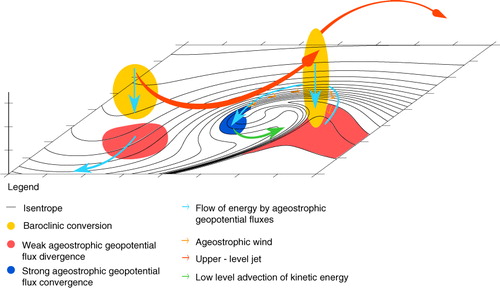
In summary, the energetics of the lower-tropospheric downstream cyclone can be illustrated schematically as in Fig. 13: ageostrophic geopotential fluxes (blue arrows) radiate KE from the mid-tropospheric zone of baroclinic generation of KE (yellow) in the warm sector to the lower troposphere and along the warm front to the tail of the bent-back front on the rearward side of the cyclone. Strong convergence of horizontal ageostrophic geopotential fluxes along the bent-back front gives rise to the low-level jet. Advection (green arrow) then spreads the KE behind the cold front.

Fig. 13.  Schematic summarizing the generation of KE in the lower troposphere by baroclinic conversion and its redistribution by ageostrophic geopotential fluxes and advection in an idealised downstream cyclone.

5.1. Limitations

The QG perspective has the advantage of its simplicity, but it involves approximations, not least the neglecting of the ageostrophic wind in the expression for KE, which leads to significant deviations from the actual values of KE and its tendencies. This becomes particularly evident when terms are integrated along trajectories. For trajectories forming the low-level jet at day 6 hour 18 we find that the source terms in eq. (1) underestimate the average increase of QG KE by 521 J m⁻³ (i.e. slightly more than 100%). Neglecting the ageostrophic wind in the expression for KE causes an overestimation of the actual wind by roughly 10 m s⁻¹, which leads to an overestimation of KE by 400 J m⁻³ and therefore likely accounts for the major part of the discrepancy. Thus, it is important not to draw detailed quantitative conclusions from our analysis but to emphasise the qualitative findings instead, which are valid beyond the QG framework. This was verified using the full-wind eddy KE equation (Orlanski and Katzfey, 1991), which confirmed our findings, but comes at the expense of additional terms arising due to the interaction of the eddy and the zonal flow.

Furthermore, the absence of moisture and of a boundary layer parameterisation impacts on the cyclone development, in particular the strength of the low-level jet. By adding a boundary layer parametrisation we expect a weakening of the low-level jet due to surface drag. On the other hand if moisture was included, diabatic effects may speed-up and enhance cyclone development and strengthen the low-level jet. Such a diabatic enhancement of the low-level jet in a secondary cyclogenesis event was reported by Grønås (1995). Additional simulations including moisture and the effect of latent heat release by condensation (Schemm et al., 2013) revealed a qualitatively similar, albeit more intense and faster, energetic evolution. In particular the formation of the low-level jet by ageostrophic geopotential flux convergence occurs in the same manner.

5.2. Outlook

It remains the subject of further investigations to study in more detail the low-level KE and the generality of the findings of this study for cyclones that differ from the Shapiro-Keyser conceptual model. In recent years channel simulations using realistic physics have become popular, for instance to characterise life-cycle differences of cyclones in different flow regimes, (e.g. Davis, 2010). Also such simulations became a valuable tool to improve our understanding of the ventilation of the boundary layer by baroclinic eddies (Sinclair et al., 2008) and moisture transport in extratropical cyclones (Boutle et al., 2010; Boutle et al., 2011). Thus, it will be useful to successively add more realism to our channel simulations by the introduction of turbulent surface fluxes, the inclusion of moisture and a convection scheme, and to assess the influence of these processes on the energetic development of the downstream cyclone. Furthermore, confluent and diffluent background flows were found to be decisive for the evolution of certain frontal structures (Schultz and Zhang, 2007). Investigations of cyclone development in zonally varying flows will help to understand the different evolutions of the Norwegian and Shapiro-Keyser type cyclones from an energetics perspective.

6. Acknowledgments

L. Papritz acknowledges support by ETH Research Grant CH2-01 11-1 and S. Schemm acknowledges funding from the Swiss National Science Foundation (Project 200021-130079). We thank Heini Wernli (ETH Zürich) for insightful discussions and are grateful for detailed comments on the manuscript. Also we would like to thank Stephan Pfahl (ETH Zürich) for carefully reviewing an early draft. The comments of two anonymous reviewers helped to strengthen our presentation, and these are gratefully acknowledged.

Notes

¹Translation from German to English by the authors.

²Local energetics analysis has mostly been performed with pressure coordinates. Therefore, we stick to the traditional nomenclature, even though ageostrophic pressure flux would be more appropriate here.

³1 PVU=10⁻⁶ m² s⁻¹ K kg⁻¹

⁴We nevertheless look at them in a forward-in-time direction and therefore denote their position at day 4 hour 12 as their endpoint.

⁵The discrepancy between the total increase of KE and the sum of the source terms in the KE equation by about 30 J m⁻³ is mainly due to the QG approximation (also see Section 5.1).

References

- Boutle I. A. Beare R. J. Belcher S. E. Brown A. R. Plant R. S. The moist boundary layer under a mid-latitude weather system. Boundary-Layer Meteorol. 2010; 134: 367–386. 10.3402/tellusa.v65i0.19539.
- Boutle I. A. Belcher S. E. Plant R. S. Moisture transport in midlatitude cyclones. Quart. J. Roy. Meteor. Soc. 2011; 137: 360–373. 10.3402/tellusa.v65i0.19539.
- Davis C. A. Simulations of subtropical cyclones in a baroclinic channel model. J. Atmos. Sci. 2010; 67: 2871–2892. 10.3402/tellusa.v65i0.19539.
- Decker S. G. Martin J. E. A local energetics analysis of the life cycle differences between consecutive, explosively deepening, continental cyclones. Mon. Wea. Rev. 2005; 133: 295–316. 10.3402/tellusa.v65i0.19539.
- Eady E. T. Long waves and cyclone waves. Tellus. 1949; 1: 33–52. 10.3402/tellusa.v65i0.19539.
- Grønås S. The seclusion intensification of the new year's day storm 1992. Tellus A. 1995; 47: 733–746. 10.3402/tellusa.v65i0.19539.
- Holton, J. R. 2004. Synoptic-scale motions I: quasi-geostrophic analysis. In: An Introduction to Dynamic Meteorology. Elsevier Academic Press: Amsterdam, pp. 139–176.
- Lackmann G. M. Keyer D. Bosart L. F. Energetics of an intensifying jet streak during the experiment on rapidly intensifying cyclones over the atlantic (ERICA). Mon. Wea. Rev. 1999; 127: 2777–2794.
- Lorenz E. N. Available potential energy and the maintenance of the general circulation. Tellus. 1955; 7: 157–167. 10.3402/tellusa.v65i0.19539.
- Margules, M. 1905. Über die Energie der Stürme. In: Jahrbücher der k.k. Central-Anstalt für Meteorologie und Erdmagnetismus. Vol. 48 (40), K.K. Hof- und Staatsdruckerei, Wien, pp. 1–26. Appendix.
- O'Gorman P. A. Schneider T. Energy of midlatitude transient eddies in idealized simulations of changed climates. J. Climate. 2008; 21: 5797–5806. 10.3402/tellusa.v65i0.19539.
- Olson J. B. Colle B. A. A modified approach to initalize an idealized extratropical cyclone within a mesoscale model. Mon. Wea. Rev. 2007; 135: 1614–1624. 10.3402/tellusa.v65i0.19539.
- Oort A. H. On estimates of the atmospheric energy cycle. Mon. Wea. Rev. 1964; 92: 483–493.
- Oort A. H. Peixóto J. P. The annual cycle of the energetics of the atmosphere on a planetary scale. J. Geophys. Res. 1974; 79: 2705–2719. 10.3402/tellusa.v65i0.19539.
- Orlanski I. Chang E. K. M. Ageostrophic geopotential fluxes in downstream and upstream development of baroclinic waves. J. Atmos. Sci. 1993; 50: 212–225.
- Orlanski I. Katzfey J. The life cycle of a cyclone wave in the Southern Hemisphere. Part I: eddy energy budget. J. Atmos. Sci. 1991; 48: 1972–1998.
- Orlanski I. Sheldon J. P. A case of downstream baroclinic development over western North Africa. Mon. Wea. Rev. 1993; 121: 2929–2950.
- Orlanski I. Sheldon J. P. Stages in the energetics of baroclinic systems. Tellus A. 1995; 47: 605–628. 10.3402/tellusa.v65i0.19539.
- Pedlosky, J. 1987. Geostrophic energy equation and available potential energy. In: Geophysical Fluid Dynamics. Springer-Verlag: New York, pp. 368–374.
- Schemm S. Wernli H. Papritz L. Warm conveyor belts in idealized moist baroclinic wave simulations. J. Atmos. Sci. 2013; 70: 627–652. 10.3402/tellusa.v65i0.19539.
- Schultz D. M. Zhang F. Baroclinic development within zonally – varying flows. Quart. J. Roy. Meteor. Soc. 2007; 133: 1101–1112. 10.3402/tellusa.v65i0.19539.
- Shapiro, M. A and Keyser, D. 1990. Fronts, jet streams and the tropopause. In: Extratropical Cyclones. The Erik Palmen Memorial Volume. C. W.Newton and E. O.Holopainen, American Meteorological Society: BostonUSA, pp. 167–191.
- Sinclair V. A. Gray S. L. Belcher S. E. Boundary-layer ventilation by baroclinic life cycles. Quart. J. Roy. Meteor. Soc. 2008; 134: 1409–1424. 10.3402/tellusa.v65i0.19539.
- Steppeler J. Doms G. Schättler U. Bitzer H. W. Gassmann A. co-authors. Meso-gamma scale forecasts using the nonhydrostatic model LM. Meteor. Atmos. Phys. 2003; 82: 75–96. 10.3402/tellusa.v65i0.19539.
- Wernli H. Davies H. C. A Lagrangian-based analysis of extratropical cyclones. I: the method and some applications. Quart. J. Roy. Meteor. Soc. 1997; 123: 467–489. 10.3402/tellusa.v65i0.19539.
- Wernli H. Shapiro M. A. Schmidli J. Upstream development in idealized baroclinic wave experiments. Tellus A. 1999; 51: 574–587. 10.3402/tellusa.v65i0.19539.