Data assimilation with correlated observation errors: experiments with a 1-D shallow water model

Abstract

Remote sensing observations often have correlated errors, but the correlations are typically ignored in data assimilation for numerical weather prediction. The assumption of zero correlations is often used with data thinning methods, resulting in a loss of information. As operational centres move towards higher-resolution forecasting, there is a requirement to retain data providing detail on appropriate scales. Thus an alternative approach to dealing with observation error correlations is needed. In this article, we consider several approaches to approximating observation error correlation matrices: diagonal approximations, eigendecomposition approximations and Markov matrices. These approximations are applied in incremental variational assimilation experiments with a 1-D shallow water model using synthetic observations. Our experiments quantify analysis accuracy in comparison with a reference or ‘truth’ trajectory, as well as with analyses using the ‘true’ observation error covariance matrix. We show that it is often better to include an approximate correlation structure in the observation error covariance matrix than to incorrectly assume error independence. Furthermore, by choosing a suitable matrix approximation, it is feasible and computationally cheap to include error correlation structure in a variational data assimilation algorithm.

• variational data assimilation
• correlated observation errors
• approximate covariance matrices
• Markov correlation structures
• eigendecompositions
• shallow water equations

1. Introduction

Data assimilation provides techniques for combining observations of atmospheric variables with a priori knowledge of the atmosphere to obtain a consistent representation known as the analysis. The weighted importance of each contribution is determined by the size of its associated errors; hence it is crucial to the accuracy of the analysis that these errors be correctly specified.

Theoretical presentations of data assimilation are usually restricted to cases where observation errors are taken to be random and unbiased. In practice, systematic observation errors are often estimated and removed from observations either in a pre-processing step or using an online bias correction system (e.g. Dee, 2005). In this article, we are concerned chiefly with the random component of observation error, and we will assume that these random errors are unbiased (have a zero mean), but may be correlated.

Observation errors can generally be attributed to four main sources:

1. Instrument noise.

2. Observation operator, or forward model error – For satellite observations, this includes errors associated with the discretisation of the radiative transfer equation and errors in the mis-representation of gaseous contributors.

3. Representativity error – This is present when the observations can resolve spatial scales or features in the horizontal or vertical that the model cannot. For example, a sharp temperature inversion can be well-observed using radiosondes but cannot be represented precisely with the current vertical resolution of atmospheric models.

4. Pre-processing – For example, if we eliminate all satellite observations affected by clouds and some cloud-affected observations pass through the quality control, then one of the assimilation assumptions is violated and the cloudy observations will contaminate all satellite channels that are influenced by the cloud. It is reasonable to assume that instrument errors are independent and uncorrelated. However, the other three sources of error result in observation error correlations.

Observation error correlations may be inter-channel error correlations (for satellite observations) or spatial correlations associated with an observation footprint (the region of atmosphere observed) e.g. horizontal, vertical, along a weather radar ray path etc. Temporal correlations are excluded from this work, although in principle temporal correlations (e.g. between successive observations using the same instrument) could be treated using an enlarged version of the observation error covariance matrix where the time dimension was also modelled. Here we also exclude correlations between observation errors for different instrument types, so the observation error covariance matrix can be considered block diagonal, with each block corresponding to a different instrument type.

Quantifying observation error correlations is not a straightforward problem because they can only be estimated in a statistical sense, not observed directly. A particular issue is that the distinction between biased and correlated errors can be blurred in practical contexts. For example, if we take a series of correlated samples, the series will tend to be smoother than a series of independent samples, with adjacent and nearby values more likely to be similar than a series of independent samples. Hence, in practical situations it would be easy for a sample from a correlated distribution with a zero mean to be interpreted as a biased independent sample (Wilks, 1995, section 5.2.3).

Nevertheless, attempts have been made to quantify error correlation structure for a few different observation types such as Atmospheric Motion Vectors (Bormann et al., 2003) and satellite radiances (Sherlock et al., 2003; Stewart et al., 2009; Bormann and Bauer, 2010; Bormann et al., 2010; Stewart, 2010; Stewart et al., 2012). Using diagnosed correlations such as these in an operational assimilation system is far from straightforward: early attempts by the UK Met Office using IASI and AIRS data have resulted in conditioning problems with the 4D-Var minimisation (Weston, 2011).

Due to the large number of observations, the computational demands of using observation error correlations appear to be significant. However, the size of the matrices to be stored may be reduced if the observation error covariance matrix has a block-diagonal structure, with (uncorrelated) blocks corresponding to different instruments or channels. For each block, if the observation sub-vector is of size p then the observation error covariance sub-matrix contains (p ²+p)/2 independent elements. When observations have independent errors, i.e. the errors are uncorrelated, (p ²−p)/2 of these elements are zero, and we only need represent p elements. For relatively small p, using full observation covariance sub-matrices appears feasible, although a form of regularisation may be required to overcome ill-conditioning (e.g. the recent work of Weston (2011)). However, for large p, for example when dealing with spatial correlations, another approach is required.

In current operations, observation errors are usually assumed uncorrelated. In most cases, to compensate for the omission of error correlation, the observation error variances are inflated so that the observations have a more appropriate lower weighting in the analysis (e.g. Collard, 2004). The assumptions of zero correlations and variance inflation are often used in conjunction with data thinning methods such as superobbing (Berger and Forsythe, 2004). Superobbing reduces the density of the data by averaging the properties of observations in a region and assigning this average as a single observation value. Under these assumptions, increasing the observation density beyond some threshold value has been shown to yield little or no improvement in analysis accuracy (Liu and Rabier, 2003; Berger and Forsythe, 2004; Dando et al., 2007). Stewart et al. (2008) and Stewart (2010) showed that the observation information content in the analysis is severely degraded under the incorrect assumption of independent observation errors. Such studies, combined with examples demonstrating that ignoring correlation structure hinders the use of satellite data [e.g. constraining channel selection algorithms (Collard, 2007)], suggest that error correlations for certain observation types have an important role to play in improving numerical weather forecasting. Indeed, the inclusion of observation error correlations has been shown to increase the accuracy of gradients of observed fields represented in the analysis (Seaman, 1977). Furthermore, retaining even an approximate error correlation structure shows clear benefits in terms of analysis information content (Stewart et al., 2008; Stewart, 2010).

Approximating observation error correlations in numerical weather prediction (NWP) is a relatively new direction of research but progress has been made. Healy and White (2005) used circulant matrices to approximate symmetric Toeplitz observation error covariance matrices. Results showed that assuming uncorrelated observation errors gave misleading estimates of information content, but using an approximate circulant correlation structure was preferable to using no correlations. Fisher (2005) proposed giving the observation error covariance matrix a block-diagonal structure, with (uncorrelated) blocks corresponding to different instruments or channels. Individual block matrices were approximated by a truncated eigendecomposition. The method was shown to be successful in representing the true error correlation structure using a subset of the available eigenpairs. However, spurious long-range correlations were observed when too few eigenpairs were used.

In this article, we carry out numerical experiments using incremental variational assimilation (Section 2) to address the following questions: Is it better to model observation error correlation structure approximately than not at all? and Is it computationally feasible to model observation error correlations? We use identical twin experiments so that a ‘truth’ trajectory is available and we are able to consider analysis errors explicitly. We specify two ‘true’ correlated observation error covariance matrices that we use to simulate synthetic observation errors, described in Section 3. However, in the variational minimisation, we use approximate observation error correlation structures to compute the cost function, with the aim that these approximations will provide more accurate analyses than incorrectly assuming uncorrelated errors, without a large increase in computational cost. The approximations chosen include diagonal matrices with inflated variances (Collard, 2004), a truncated eigendecomposition (Fisher, 2005), and a Markov matrix (Sections 3.2–3.4). The Markov matrix has not been applied in this context before and has the advantage of a tri-diagonal inverse.

The experiments are carried out using a 1-D, irrotational, non-linear shallow water model (SWM) described in Section 4. The experimental design is given in Section 5, and analysis error measures are discussed in Section 6. The results (Sections 7, 8 and 9) show that including some correlation structure, even a basic approximation, often produces a smaller analysis error than using a diagonal approximation. We conclude (Section 10) that it is computationally feasible and advantageous for analysis accuracy to include approximate observation error correlations in data assimilation. These encouraging results in a simple model should be investigated further for the potential improvement of operational assimilation systems.

2. Variational assimilation

Consider a discretised representation of the true state of the atmosphere , at time t _i , where n is the total number of state variables. The analysis used in NWP will consist of the same model variables as this discretisation and must be consistent with the first guess or background field and the actual observations. The background field, , is valid at initial time t ₀ and is usually given by a previous forecast. Observations are available at a sequence of times t _i and are denoted , where p _i is the total number of measurements available at time t _i . The background state and observations will be approximations to the true state of the atmosphere,1 2 where are the background errors valid at initial time, are the observation errors at time t _i , and h _i is the, possibly non-linear, observation operator mapping from state space to measurement space at time t _i ; for example, a radiative transfer model which simulates radiances from an input atmospheric profile. The errors are assumed unbiased and mutually independent, and also to have covariances and .

The objective of variational assimilation is to minimise the cost function,3 subject to the strong constraint that the sequence of model states must also be a solution to the model equations,4 where x _i is the model state at time t _i and is the non-linear model evolving x ₀ from time t ₀ to time t _i . The strong constraint given by eq. (4) implies the model is assumed to be perfect.

The cost function [eq. (3)] measures the weighted sum of the distances between the model state x ₀ and the background at the start of the time interval t ₀ and the sum of the observation innovations computed with respect to the time of the observation. Variational assimilation therefore provides an initial condition such that the forecast best fits the observations within the whole assimilation interval.

Incremental assimilation (Courtier et al., 1994), reduces the cost of the algorithm by approximating the full non-linear cost function [eq. (3)] by a series of convex quadratic cost functions. The minimisation of these cost functions is constrained by a linear approximation M to the non-linear model m [eq. (4)]. Each cost function minimisation is performed iteratively and the resultant solution is used to update the non-linear model trajectory. Full details of the procedure are described by Lawless et al. (2005) and Stewart (2010). We summarise the algorithm here, denoting k as iteration number and as the full non-linear solution valid at time t _i and the k-th iteration.

At the first time step (k=0) define the current guess .

Loop over k:

(1) Run the non-linear model [eq. (4)] to calculate at each time step i.

(2) Calculate the innovation vector for each observation

(3) Start the inner loop minimisation. Find the value of that minimises the incremental cost function5 subject towhere H _i is the linearisation of the observation operator h _i and is the linearisation of the model . Both of these linearisations are around the current state estimate (the non-linear model trajectory satisfying when ).

(4) Update the guess field using

(5) Repeat outer loop (Steps 2–5) until the desired convergence is reached.

In our implementation, the conjugate gradient method (Golub and van Loan, 1996, section 10.2) is used to carry out the inner loop minimisation to solve eq. (5). The maximum number of outer and inner loops performed is 20 and 200, respectively. The outer and inner loops are terminated once the following criteria are satisfied. For the outer loop, we require that (Lawless and Nichols, 2006)6 where the superscripts indicate the outer loop iteration index. For the inner loop, we require that7 where the subscripts 0, q indicate the inner loop iteration index and k indicates the outer loop iteration index. With these stopping criteria and tolerance values, we expect the converged solution of the minimisation to be accurate to approximately two decimal places (Gill et al., 1981, section 8.2; Stewart, 2010).

3. Observation error covariance matrices

This article describes incremental variational assimilation experiments using approximate forms of observation error covariance matrices to take account of correlated observation errors in the minimisation. In Section 3.1, we describe the ‘true’ error covariance structures we use to simulate synthetic observation errors. In Sections 3.2–3.4, we explain the choice of the various approximate forms of observation error covariance matrix we employ in the cost function. The goal is that these choices will improve the accuracy of the analysis and have only a modest computational burden.

3.1. True error covariance structures

For our experiments, we use a 1-D spatial distribution of observations, with a regular spacing between the observations. Observation errors are assumed correlated in space only (no temporal correlations). We use two different forms of true observation error covariance structure, R _t . We make use of the general decomposition of an observation error covariance matrix R into a diagonal variance matrix and a correlation matrix such that8 so that we may vary the observation error variance and correlation structure separately. Note that if C=I then R is diagonal and D is the diagonal matrix of error variances.

In Experiments 1 and 3 we use a true error correlation matrix with a Markov distribution, C _M , given by9 where m is the spatial separation and mis the length scale. The Markov matrix is the resultant covariance matrix from a first-order autoregression process, (Wilks, 1995) and is discussed in more detail in Section 3.3.

In the second experiment the true error correlation structure follows a SOAR (second-order autoregressive) distribution. The SOAR error covariance matrix is given by10 The SOAR matrix is an idealised correlation structure that is often used to model background error correlation structures in the horizontal (e.g. Ingleby, 2001). It is commonly employed in preference to a Gaussian structure because its distribution has longer tails, better at matching empirical estimates and is better conditioned for inversion (Haben, 2011; Haben et al., 2011).

3.2. Diagonal approximation

The diagonal approximation that we use in our experiments is commonly employed operationally. Diagonal matrices are simple and numerical efficient: In incremental variational assimilation, inverse observation error covariance matrices are required for matrix-vector products in evaluating the cost function and gradient, where N is the number of assimilation time steps. When an observation error covariance matrix is diagonal, its inverse will also be diagonal, resulting in very inexpensive matrix-vector products.

The simplest diagonal approximation of an error covariance matrix is taking the diagonal equal to the true variances. However, by ignoring entirely the correlated component of the observation error, the observations will be overweighted in the analysis because they will appear more informative than they truly are. Therefore, in order to compensate for the lack of correlation, a diagonal approximation given by the diagonal of the true matrix scaled by an inflation factor is used (Hilton et al., 2009). This reduces the weighting of the observations in the analysis. The diagonal approximation is now in the form11 where d _i is the real, positive inflation factor for variance .

In our experiments, the diagonal matrix representations are a diagonal matrix of the true error variances [ for in eq. (11)], and scalar multiples of this matrix [ for some scalar , in eq. (11)]. The scalar multiples are chosen to be between two and four, in line with our earlier 3D-Var information content results (Stewart et al., 2008; Stewart, 2010) and results given in Collard (2004). These showed that a two–four times variance inflation was preferable to a simple diagonal approximation when observation and background error correlations were both present; but when there were correlated observation errors and uncorrelated background errors, a simple diagonal approximation performed better than variance inflation.

3.3. Markov matrix

The second approximate form of matrix that we employ is a Markov matrix. This is a novel choice that has not previously been reported in the literature for observation error covariance approximation. The (i, j)th element of a general Markov matrix, R, is given by12 where σ ² is the observation error variance, and 0≤ρ≤1 is a parameter describing the strength of the correlations. This matrix has a tri-diagonal inverse (Rodgers, 2000),13 The storage needed for reconstructing matrix [eq. (13)] is limited to the value of ρ, and the number of operations involved in a matrix-vector product using a tri-diagonal matrix is the same order as that using a diagonal matrix. Therefore, calculating the cost function using the Markov matrix approximation is a possibility for operational assimilation.

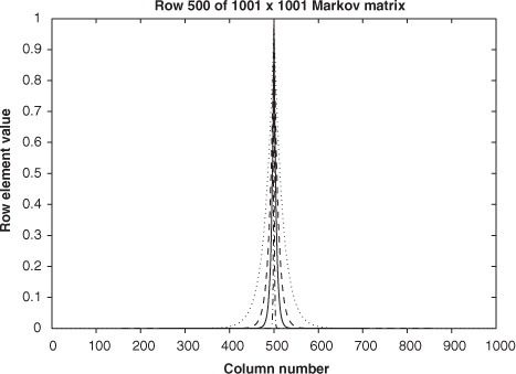
In our experiments, we let , as in eq. (9). The Markov matrix representations are Markov structured matrices with length scales m, m and m, i.e. double, the same as, half, and a tenth of the true length scale. These values are chosen to represent different levels of error dependence. In Fig. 1, the central row of each Markov matrix is plotted. Note that as the length scale decreases, the thickness of the central correlation band decreases. We also test the Markov matrix representation for the case where L _R is small enough that for ; this should produce the same result as using the diagonal approximation with the true error variances, and is a continuity test on our system.

Fig. 1 Middle row of a 1001×1001 Markov matrix, (9). Dash–dot line L _R =0.01m, full line L _R =0.05m, dashed line L _R =0.1m and dotted line L _R =0.2 m.

3.4. Eigendecomposition matrix

Starting from the general covariance decomposition [eq. (8)], Fisher (2005) proposed that the observation error covariance matrix be approximated using a truncated eigendecomposition of the error correlation matrix C,14 where is an (eigenvalue, eigenvector) pair of C, K is the number of leading eigenpairs used in the approximation, and is chosen such that trace (R)=trace (D). This ensures that there is no mis-approximation of the total error variance, since trace ()=trace (D). A formula for may be computed as15 using the additive property of the trace function. The inverse of eq. (14) is easily obtainable and is given by16 The representation [eq. (14)] allows the retention of some of the true correlation structure, with the user choosing how accurately to represent the inverse error covariance matrix [eq. (16)] through the choice of K. Care must be taken to ensure numerical stability (for example choosing K such that is never too small).

In Fisher (2005) the leading eigenpairs of C are found using the Lanczos algorithm. In our experiments, the leading eigenpairs needed for the representation are pre-computed using the MATLAB function eigs() (MathWorks, 2009) which uses an implicitly restarted Arnoldi method (Sorensen, 1992; Lehoucq and Sorensen, 1996).

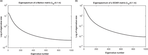
By studying the eigenspectra of the true error correlation matrices we can estimate how many eigenpairs are needed for a good representation. The eigenspectra of a Markov matrix and a SOAR matrix, both of size 1001×1001, with length scale m and spatial separation m, are plotted in Fig. 2. The plots show that the eigenvalue size declines sharply as the eigenvalue number increases. The condition number (ratio of largest to smallest eigenvalue) for the Markov matrix is 400 and for the SOAR matrix is 4.8×10⁵. After 100 eigenvalues, 80 and 99% of the overall uncertainty is represented for the Markov and SOAR matrix respectively – uncertainty percentages are calculated using (sum of eigenvalues used)/(sum of all eigenvalues or trace of matrix)×100%. Therefore, we use 100 eigenpairs as an empirical upper limit to the number of eigenpairs used in the assimilation.

Fig. 2 (a) Eigenspectrum of a 1001×1001 Markov error correlation matrix; (b) Eigenspectrum of a 1001×1001 SOAR error correlation matrix.

The number of eigenpairs we use in our approximations are K=10, K=20, K=50 and K=100. This represents 1, 2, 5 and 10% of the total number of eigenpairs. An eigendecomposition (ED) approximation using the full number of eigenpairs K=1001 is equivalent to using the true error correlation matrix in the system. Obviously using all the eigenpairs is an expensive procedure and would not be attempted operationally. However, in these smaller dimensioned experiments, knowing the performance of the assimilation under the true error correlation matrix allows us to quantify the success of an assimilation using an approximated correlation matrix relative to the truth. We therefore also run the assimilation using the ED approximation with the full number of eigenpairs.

4. Shallow water model

In this section we describe the forecast model used in our experiments. This is a 1-D, non-linear, SWM system describing the irrotational flow of a single-layer, inviscid fluid over an object. The SWM has been used for a variety of assimilation experiments e.g. Lawless et al. (2005, 2008); Katz et al. (2011); Steward et al. (2012). As an idealised system, it allows clearer understanding of the results without the obfuscating complexity of a more realistic system.

The continuous equations describing 1-D shallow water flow are given by17 18 on the domain , , where19 and is the height of the bottom orography, u is the fluid velocity, φ=gh _f is the geopotential where g is the gravitational acceleration and h _f >0 is the depth of fluid above the orography. The spatial boundary conditions are taken to be periodic, so that at any time ,The non-linear shallow water equations are discretised using a two-time-level semi-implicit, semi-Lagrangian scheme, described by (Lawless, 2001; Lawless et al., 2003).

The experiments in this article model a flow field described in Houghton and Kasahara (1968) in which shallow water motion is forced by some orography. Using the shallow water eqs. (17) and (18), we consider a fluid at rest when t<0, with the geopotential equal to , where φ ₀ is a constant. At t=0 the fluid is set in motion with a constant velocity u ₀ at all grid points, causing a wave motion to develop outwards from the obstacle in the fluid. The solution close to the object becomes a steady state solution (Lawless et al., 2003). We restrict the fluid motions to be not too highly non-linear so as to keep our assumptions of linearity as valid as possible. We use a periodic domain where the boundaries are at a sufficient distance from the obstacle to ensure any propagating wave motions in the vicinity of the obstacle respect the asymptotic conditions.

The data used in the experiment is based on Case A in Houghton and Kasahara (1968). We consider a 1-D spatial domain between [0,10m] equally divided into 1001 grid points with spatial step m. The height of the obstacle in the fluid is given bywhere h _C is the maximum height of the obstacle and a is half the length over which the base of the obstacle extends. The values of a and h _C are set as: , . The temporal domain is 100 time steps with step size s. At t=0 the initial velocity is u₀=0.1 ms⁻¹, and the geopotential is where g=10 ms⁻².

5. Twin experiments

Our numerical experiments are performed using an assimilation-forecast system based on an incremental variational assimilation system implemented for the SWM of Section 4. In order to assess the impact of modelling correlated observation error structure, we use different approximations to the observation error covariance matrix in the cost function, as discussed in Section 3: diagonal approximations, Markov approximations and ED approximations. By keeping all other variables the same, any changes in the analysis trajectory can be attributed to the specification of the observation errors. In practice, such an approach is not always possible since the true error covariance matrix is rarely known explicitly. The 1-D construction of the SWM means we are considering error correlations between observations in the horizontal. However, the techniques we are using could easily be translated to a 1-D vertical profile, such as the radiance profiles used in 1D-Var. Therefore our assimilation tests will remain independent of any discussion on issues of spatial resolution or horizontal thinning.

An identical twin experiment is performed by running the non-linear SWM forward in time from the initial conditions described in Section 4, to generate a true model solution at each assimilation time step, . This is known as the truth trajectory. Observations of fluid velocity u and geopotential φ are sampled from the truth trajectory. It is assumed that there is an observation at each grid point, and after every 10 time steps, i.e. 10 sets of 1001 observations in total; this density was chosen to represent a very well-observed system. Random noise with multivariate normal distribution is added as observation error. The errors in the u and φ observations are assumed mutually uncorrelated so that the observation error vectors for the u and φ fields may be generated independently. The correlation structures for the errors are given in Section 3.1. For most of the experiments, the observation error variances are set at 0.0004 m²s⁻² for u observations and 0.04 m⁴s⁻⁴ for φ observations. Thus the standard deviation of the noise corresponds to 20% of the mean field value.

The initial background is taken as the initial truth trajectory plus random noise from a normal distribution with mean zero and covariance matrix B _t . Experiments 1 and 2 are run with uncorrelated background errors where the background error variances are set at 0.0002 m²s⁻² for u observations and 0.02 m⁴s⁻⁴ for φ observations. In Experiment 3, we choose the background error variances to be the same as in the other experiments. However, for this experiment, the errors are spatially correlated, with a Markov correlation structure, specified as in eq. (9) with m and L _R =0.1m.

An incremental data assimilation algorithm is then run using these observation and background data, with the covariances used in the calculation of the cost function taken to be B _t for the background error covariance and R _f (an approximate covariance structure) for the observation error covariance. The time window for the assimilation is 100 model time steps. The assimilation finds an analysis valid at initial time t=0, for each model grid point. We then integrate the analysis forward in time to give an updated forecast. The accuracy of the resulting analysis and forecast can be evaluated using the error measures described in the next section. Note that we perform only one analysis and forecast – we perform no cycling in these experiments.

6. Analysis error measures

We now describe the diagnostics used to evaluate the success of each approximation. The assimilation is run using different approximations R _f to the true error covariance matrix R _t . We illustrate the comparative behaviour of the assimilation under different approximations by comparing:

• Error 1 (E1): The norm of the analysis error with respect to the true solution

20 where x ^t is the true solution of the original model run from which the observations are sampled, and is the converged solution to the assimilation problem when the approximation R _f is used in calculating the cost function, but the observation errors themselves are sampled using the true error covariance R _t ;

• Error 2 (E2): The percentage norm of the analysis error in the converged solution relative to the norm of the true converged solution

21 where is the true converged solution to the assimilation problem when the true error covariance matrix R _t is used both in calculating the cost function and in sampling the observation errors.

Errors E1 and E2 provide us with information on the closeness of different analyses. Since the magnitude of the φ field is an order larger than that of the u field, we produce separate error norms [eqs. (20) and (21)] for u and φ to avoid changes in the u field being overshadowed by changes in the φ field.

7. Experiment 1: Markov error correlation structure

In our first experiment we investigate the impact on analysis accuracy of using a diagonal matrix, a Markov matrix and an ED matrix to represent a Markov error correlation structure. The analysis errors E1 and E2 at the start of the assimilation window (t=0) for different approximations to a Markov error correlation structure are given in Table 1 and 2 for u and φ, respectively.

Table 1. Analysis errors in u field at t=0 for different approximations to a Markov error covariance matrix ()

Approximation	E1:		E2 (%)
Truth	0.20	0	0
Diagonal	0.30	0.23	7.2
2×diagonal	0.31	0.23	7.2
4×diagonal	0.31	0.24	7.5
Markov (L R =0.2)	0.21	0.06	1.9
Markov (L R =0.1)	0.20	0	0
Markov (L R =0.05)	0.21	0.05	1.6
Markov (L R =0.01)	0.27	0.18	5.6
ED (K=10)	0.28	0.19	5.9
ED (K=20)	0.28	0.19	5.9
ED (K=50)	0.25	0.15	4.7
ED (K=100)	0.23	0.10	3.1

Table 2. Analysis errors in φ field at t=0 for different approximations to a Markov error covariance matrix ()

Approximation	E1:		E2 (%)
Truth	2.35	0	0
Diagonal	3.61	3.04	4.9
2×diagonal	3.85	3.32	5.3
4×diagonal	4.11	3.61	5.8
Markov (L R =0.2)	2.41	0.54	0.9
Markov (L R =0.1)	2.35	0	0
Markov (L R =0.05)	2.42	0.67	1.1
Markov (L R =0.01)	3.06	2.27	3.6
ED (K=10)	3.97	3.25	5.2
ED (K=20)	3.80	3.03	4.8
ED (K=50)	3.33	2.39	3.8
ED (K=100)	2.77	1.56	2.5

The error in the background field is for the u field and for the φ field. We can see in Table 1 and 2 that in all cases the approximation results in an improvement to the background field. Using the true error covariance matrix, i.e. a Markov matrix with length scale L _R =0.1m, produces the smallest analysis errors; the percentage error E2 is zero for this matrix because R _t =R _f Using a diagonal matrix approximation results in the largest analysis errors.

Using a Markov approximation with double (L _R =0.2 m) or half (L _R =0.05 m), the true length scale results in a small E2 error of less than 2% for the u and φ fields. This implies that choosing the exact length scale is not essential to producing accurate results. Also, using a Markov matrix approximation with length scale between L _R =0.2 m and L _R =0.05 m results in a smaller E2 error than that of an ED approximation using 100 eigenpairs. Using more eigenpairs in the ED approximation produces a more accurate analysis, but at greater computational expense because additional eigenpairs must be stored and used in cost function computations. We can therefore infer that although using more eigenpairs is beneficial, a Markov approximation using an approximate length scale is cheaper and more effective. In the next section, we will see if the same conclusions are drawn when the true error covariance matrix follows a non-Markov distribution.

It is worth noting that using an ED approximation with a small number of eigenpairs can generate a smaller analysis error than when a diagonal approximation is used and is comparable with a weakly correlated Markov approximation. For example, a diagonal matrix approximation results in an E2 error of 7.2% in the u field compared to a 5.9% error under an ED matrix with 10 eigenpairs and a 5.6% error under a Markov matrix with length scale L _R =0.01m. Combined with the results for a Markov matrix approximation, this implies that it is often better to include some correlation structure, even if it is a weak approximation, than none at all.

Similar tests were performed for different observation frequencies. We found that using more frequent observations resulted in a small improvement in E2 for the three matrix approximations tested: a diagonal matrix, a Markov matrix with L _R =0.05 m and an ED matrix with K=50. Increasing the frequency of observations had the biggest impact on the diagonal approximation. Nevertheless, even when there were observations at every time step (100 observation sets) the error E2 under a diagonal approximation was still significantly larger (5.7%than when a Markov (1.3%) and an ED approximation (3.4%) were used.

In the next section we will extend the experiments performed here to a different choice of true error correlation structure.

8. Experiment 2: SOAR error correlation structure

In this section we consider the effect of our choice of the true observation error correlation structure. In Experiment 1, the true error correlation matrix was generated from a Markov distribution [eqs. (8) and (9)]. We now change the true correlation matrix to represent a SOAR distribution with length scale L _R =0.1m [eqs. (8) and (10)]. The matrix representations used to approximate this correlation structure are the same as those used in Experiment 1. Using a SOAR matrix will allow us to determine whether the Markov approximation also minimises analysis error when the true correlation structure is not in Markov form, and how well the ED and diagonal approximations perform in comparison.

The analysis errors E1 and E2 at t=0 for the different approximations to the SOAR error covariance matrix are given in Table 3 and 4, for u and φ respectively. Comparing the results to Table 1 and 2, we observe that the qualitative nature of the errors is very similar. For example, using the true error covariance matrix structure results in the smallest errors and diagonal approximations result in the largest errors. The approximations resulting in the smallest analysis errors are a Markov matrix with length scale L _R =0.2 m and an ED matrix using 100 eigenpairs. It is intuitive that a Markov matrix with a longer length scale is preferable, because of the longer tails in a SOAR function. The E2 error in the u field is also small for Markov approximations with length scale between L _R =0.2 m and L _R =0.05 m, compared to a 9.4% error when a 4×diagonal approximation is used. Inflated diagonal approximations perform slightly worse than a simple diagonal approximation; this is in line with the information content results in Stewart (2010), when the background errors were uncorrelated.

Table 3. Analysis errors in u field at t=0 for different approximations to a SOAR error covariance matrix ()

Approximation	E1:		E2 (%)
Truth	0.11	0	0
Diagonal	0.31	0.28	8.8
2×diagonal	0.32	0.29	9.1
4×diagonal	0.32	0.30	9.4
Markov (L R =0.2)	0.13	0.07	2.2
Markov (L R =0.1)	0.15	0.11	3.4
Markov (L R =0.05)	0.18	0.15	4.7
Markov (L R =0.01)	0.27	0.25	7.8
ED (K=10)	0.26	0.24	7.5
ED (K=20)	0.23	0.20	6.3
ED (K=50)	0.15	0.11	3.4
ED (K=100)	0.13	0.07	2.2

Table 4. Analysis errors in φ field at t=0 for different approximations to a SOAR error covariance matrix ()

Approximation	E1:		E2 (%)
Truth	0.57	0	0
Diagonal	3.36	3.32	5.3
2×diagonal	3.59	3.55	5.7
4×diagonal	3.99	3.95	6.3
Markov (L R =0.2)	0.81	0.63	1.0
Markov (L R =0.1)	1.18	1.06	1.7
Markov (L R =0.05)	1.69	1.60	2.6
Markov (L R =0.01)	2.89	2.84	4.5
ED (K=10)	3.90	3.87	6.2
ED (K=20)	3.71	3.67	5.9
ED (K=50)	1.56	1.45	2.3
ED (K=100)	1.06	0.85	1.4

It is also expected that an ED matrix using 100 eigenpairs results in a very small analysis error relative to the converged solution, because as we observed in Section 3.4, 100 eigenpairs represent 99% of the overall uncertainty in the matrix. It is encouraging that an ED approximation using even fewer eigenpairs also results in an improved E2 error relative to a diagonal approximation; using 5% of the available eigenpairs results in an E2 error in the φ field of 2.3% compared to 5.3% when a diagonal approximation is used. The E1 errors in using an ED approximation to model a SOAR error covariance structure are smaller than those generated when an ED approximation was used to model a Markov error covariance structure in Experiment 1. This is because, for a SOAR error covariance matrix, more uncertainty is represented using the same number of eigenpairs; as demonstrated in the steeper gradient in Fig. 2.

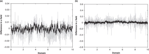
It is also interesting to look at individual analysis errors over the domain. At each grid point the analysis error is given by the difference between the true analysis and the analysis resulting from the assimilation. Figures 3 and 4 show the analysis errors in the u and φ fields at t=0 and t=50, respectively. By looking at the spread of analysis errors for the diagonal and Markov approximations, we see that the difference between the two is not uniform over the domain, i.e. in some regions, a diagonal approximation is much worse than a Markov approximation compared to the average. In real atmospheric systems, such locally larger errors may lead to severe errors in subsequent forecasts.

Fig. 3 Analysis errors in (a) u field and (b) φ field at the start of the time window. The grey line is for a diagonal approximation and the black line is for a Markov approximation with L _R =0.2m.

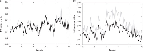
Comparing Fig. 3 to Fig. 4, we observe that as the forecast evolves the analysis errors become smoother. For the u field, the overall magnitude of the errors remains the same, but there is a reduction in error for the φ field. At the start of the time window, the diagonal approximation performs worse than the Markov approximation for both u and φ fields. At the centre of the time window, the errors in the u field for a Markov and a diagonal approximation are very similar, but for the φ field, the Markov approximation is still noticeably better. We can explain this by considering the assumptions on the SWM. The model in this assimilation is assumed perfect, and by construction is well-behaved, meaning that small errors in the analysis at t=0 will be smoothed out over time. However, for a more complex operational system, a slight error in the true analysis field at t=0 may propagate and grow with time, resulting in a modified forecast. It would therefore be interesting to extend these results to an imperfect and more poorly behaved model system.

Fig. 4 Analysis errors in (a) u field and (b) φ field at the centre of the time window, t=50. The grey line is for a diagonal approximation and the black line is for a Markov approximation with L _R =0.2m. Note that the scale in panel (b) is different from Fig. 3b.

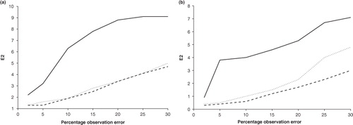
Finally in this section we study how the error in the assimilation depends on the level of noise on the observations. Previous experiments were run with the standard deviation of the noise at 20% of the mean field value; here we vary this value between 1 and 30% . The error in the assimilation is described by E2, as defined in Section 6 [eq. (21)]. A plot of this error measure vs. the percentage observation error in the u and φ field is shown in Fig. 5. We see that for all three approximations studied, the E2 error increases with the percentage observation error. In the u field, E2 increases close to linearly with noise level for the Markov and ED approximation; similarly for the φ field below 20% noise level. However, the diagonal approximation increases more rapidly with noise level in both fields, although the gradient becomes more linear as the observation errors increase. We can conclude that using a correlated matrix approximation is preferable to a diagonal one regardless of the level of observation error noise.

Fig. 5 Plot of E2 against level of observation noise for (a) u field, (b) φ field. The solid line is for the diagonal approximation, the dashed line for the ED approximation with K=50 and the dotted line for the Markov approximation with L _R =0.05m.

9. Experiment 3: correlated background errors

The previous two experiments used uncorrelated background errors and a diagonal covariance matrix B _t . We now consider the effect of correlated background errors. The true observation error structure is chosen to be the same as in Experiment 1, i.e. a Markov structure, [eq. (9) with L _R =0.1]. The background error covariance is taken to be . The background errors are modelled correctly in the experiment, i.e. the random background errors are sampled from the same distribution as is modelled in the cost function.

The analysis errors E1 and E2 at t=0 are given in Table 5 and 6, for u and φ respectively. The tables show that the different approximations to R still have an impact on the analysis accuracy when the background errors are correlated, and the impact is a similar order of magnitude to that seen in Experiment 1 (with uncorrelated background errors). As before, the diagonal approximations give some of the worst performances. However, unlike Experiment 1, variance inflation improves the results slightly. This change in behaviour with correlated vs. uncorrelated background errors is consistent with our earlier 3D-Var information content results (Stewart et al., 2008) as discussed in Section 3.2. The results using an ED approximation are mixed: for the u field the performance is only comparable to the diagonal approximations, although for the φ field the ED approximation yields better results. Fisher (2005) notes a potential problem with the eigendecomposition approach in that the approximate R matrices contain spurious correlations, although it is hoped that contributions from these spurious correlations may cancel out in the analysis. We hypothesise that the particular realisation of the observation and background noise used in this experiment has amplified this problem, although more detailed experiments beyond the scope of this article would be needed to verify this hypothesis definitively. Overall the Markov approximations provide the best results in terms of analysis accuracy (also seen in Experiment 1 and 2). Finally, we note that the detailed results seen in Experiments 1 and 2 change when background errors are correlated, but that the general conclusion that it is better to include some level of correlation structure in the observation error covariance matrix approximation than to incorrectly assume error independence still holds.

Table 5. Analysis errors in u field at t=0 for different approximations to a Markov observation error covariance matrix, with correlated background errors

Approximation	E1:		E2 (%)
Truth	0.23	0	0
Diagonal	0.30	0.19	5.7
2×diagonal	0.28	0.16	5.0
4×diagonal	0.26	0.14	4.4
Markov (L R =0.2)	0.26	0.11	3.4
Markov (L R =0.1)	0.23	0	0
Markov (L R =0.05)	0.23	0.07	2.3
ED (K=50)	0.34	0.21	6.4
ED (K=100)	0.30	0.16	5.0

Table 6. Analysis errors in φ field at t=0 for different approximations to a Markov observation error covariance matrix, with correlated background errors

Approximation	E1:		E2 (%)
Truth	1.59	0	0
Diagonal	2.07	1.37	2.2
2×diagonal	2.06	1.37	2.2
4×diagonal	2.06	1.35	2.2
Markov (L R =0.2)	1.74	0.72	1.1
Markov (L R =0.1)	1.59	0	0
Markov (L R =0.05)	1.65	0.45	0.7
ED (K=50)	1.85	0.91	1.4
ED (K=100)	1.77	0.78	1.3

10. Summary and discussion

The correct treatment of observation errors is a double problem for operational weather centres. Firstly the statistical properties of the errors are relatively unknown. Observations taken by different instruments are likely to have independent errors, but pre-processing techniques, mis-representation in the forward model, and contrasting observation and model resolutions can create error correlations. Secondly, even when good estimates of the errors can be made, it is unclear what effect their inclusion in the assimilation may have. Although the feasibility of including cross-channel correlations for satellite infra-red sounders has already been shown and seen to improve forecast skill, there were conditioning problems with the minimisation that had to be overcome (Weston, 2011). This was accomplished using matrix approximations of a similar type to those used in this article.

In this article, we developed an incremental variational data assimilation algorithm that used correlated approximations to model a simulated error correlation structure. This was applied to a 1-D SWM, and the impact of each approximation on analysis accuracy was determined. These results were encouraging but of course suffer from some limitations. The idealised perfect model system in the experiments does not have the same characteristics as an imperfect, complex NWP system. The assumption that every model variable is observed directly prohibits a direct comparison with satellite data assimilation, in which the desired atmospheric fields are non-linear combinations of the observed quantities, and observations are only available over limited regions at a given time. The choice of background error covariance matrix, B, has been specified using a functional form that is easy to calculate, rather than by collating statistics from forecast differences or an ensemble, as is more typical in operational forecasting (Bannister, 2008).

We concluded from the experiments that by choosing a suitable matrix approximation it is feasible to cheaply include some level of error correlation structure in a variational data assimilation algorithm. For different simulated observation error distributions and levels of error noise, we showed it is better to include some level of correlation structure in the observation error covariance matrix approximation than to assume incorrectly error independence. The best results were achieved using a Markov matrix approximation, and this was found to be robust to changes in true correlation form and lengthscale. While these results show promise and provide useful guidance, further development is needed to apply these ideas with real observations in operational systems. This work is already underway (Weston, 2011; Pocock et al., 2012; Stewart et al., 2012).

Acknowledgements

Laura Stewart was supported by a UK NERC PhD studentship with CASE sponsorship from the UK Met Office. Nancy Nichols and Sarah Dance were supported in part by the NERC National Centre for Earth Observation.

References

- Bannister R. N . A review of forecast error covariance statistics in atmospheric variational data assimilation. I: characteristics and measurements of forecast error covariances. Q. J. Roy. Meteorol. Soc. 2008; 134: 1951–1970.
- Berger H , Forsythe M . Satellite Wind Superobbing. 2004. Met Office Forecasting Research Technical Report, Met Office, Exeter UK, 451.
- Bormann N , Bauer P . Estimates of spatial and interchannel observation-error characteristics for current sounder radiances for numerical weather prediction. I: methods and application to atovs data. Q. J. Roy. Meteorol. Soc. 2010; 136(649): 1036–1050.
- Bormann N , Collard A , Bauer P . Estimates of spatial and interchannel observation-error characteristics for current sounder radiances for numerical weather prediction. II: application to AIRS and IASI data. Q. J. Roy. Meteorol. Soc. 2010; 136(649): 1051–1063. Online at: http://dx.doi.org/10.1002/qj.615 .
- Bormann N , Saarinen S , Kelly G , Thépaut J.-N . The spatial structure of observation errors in atmospheric motion vectors for geostationary satellite data. Mon. Weather. Rev. 2003; 131: 706–718.
- Collard A. D . On the Choice of Observation Errors for the Assimilation of AIRS Brightness Temperatures: a Theoretical Study. 2004; ECMWF Technical Memoranda, ECMWF, Reading UK, AC/90.
- Collard A. D . Selection of IASI channels for use in numerical weather prediction. Q. J. Roy. Meteorol. Soc. 2007; 133: 1977–1991.
- Courtier P , Thépaut J.-N , Holingsworth A . A strategy for operational implementation of 4D-Var, using an incremental approach. Q. J. Roy. Meteorol. Soc. 1994; 120: 1367–1387.
- Dando M. L , Thorpe A. J , Eyre J. R . The optimal density of atmospheric sounder observations in the Met Office NWP system. Q. J. Roy. Meteorol. Soc. 2007; 133: 1933–1943.
- Dee D. P . Bias and data assimilation. Q. J. Roy. Meteorol. Soc. 2005; 131: 3323–3343.
- Fisher M . Accounting for Correlated Observation Error in the ECMWF Analysis. 2005; ECMWF Technical Memoranda, ECMWF, Reading UK, MF/05106.
- Gill P , Murray W , Wright M. H . Practical Optimization. 1981; Academic Press, San Diego.
- Golub G , van Loan C. F . Matrix Computations. 1996; 3rd ed, Johns Hopkins University Press, Baltimore.
- Haben S. A . Conditioning and preconditioning of the minimisation problem in variational data assimilation. PhD Thesis, University of Reading. 2011. Online at: http://www.reading.ac.uk/maths-and-stats/research/maths-phdtheses.aspx .
- Haben S , Lawless A. S , Nichols N. K . Conditioning of incremental variational data assimilation, with application to the Met Office system. Tellus A. 2011; 63: 782–792.
- Healy S. B , White A. A . Use of discrete Fourier transforms in the 1D-Var retrieval problem. Q. J. Roy. Meteorol. Soc. 2005; 131: 63–72.
- Hilton F , Collard A , Guidard V , Randriamampianina R , Schwaerz M . Assimilation of IASI radiances at European NWP centres. Proceedings of Workshop on the Assimilation of IASI Data in NWP. 2009; UK, ECMWF: Reading. 6–8. May 2009.
- Houghton D. D , Kasahara K . Nonlinear shallow fluid flow over an isolated ridge. Comm. Pure. Appl. Math. 1968; 21: 1–23.
- Ingleby N. B . The statistical structure of forecast errors and its representation in the Met Office global 3-D variational data assimilation scheme. Q. J. Roy. Meteorol. Soc. 2001; 127: 209–231.
- Katz D , Lawless A. S , Nichols N. K , Cullen M. J. P , Bannister R. N . Correlations of control variables in variational data assimilation. Q. J. Roy Meteorol. Soc. 2011; 137: 620–630.
- Lawless A. S . Development of linear models for data assimilation in numerical weather prediction. 2001. PhD Thesis, University of Reading.
- Lawless A. S , Gratton S , Nichols N. K . An investigation of incremental 4D-Var using non-tangent linear models. Q. J. Roy. Meteorol. Soc. 2005; 131: 459–476.
- Lawless A. S , Nichols N. K . Inner-loop stopping criteria for incremental four-dimensional variational data assimilation. Mon. Weather. Rev. 2006; 134: 3425–3435.
- Lawless A. S , Nichols N. K , Ballard S. P . A comparison of two methods for developing the linearization of a shallow-water model. Q. J. Roy. Meteorol. Soc. 2003; 129: 1237–1254.
- Lawless A. S , Nichols N. K , Boess C , Bunse-Gerstner A . Using model reduction methods within incremental 4D-Var. Mon. Weather. Rev. 2008; 136: 1511–1522.
- Lehoucq R. B , Sorensen D. C . Deflation techniques for an implicitly re-started arnoldi iteration. SIAM. J. Matrix. Anal. Appl. 1996; 17: 789–821.
- Liu Z.-Q , Rabier F . The potential of high-density observations for numerical weather prediction: a study with simulated observations. Q. J. Roy. Meteorol. Soc. 2003; 129: 3013–3035.
- Pocock J. A , Dance S. L , Lawless A. S , Nichols N. K , Eyre J . Representativity error for temperature and humidity using the Met Office high resolution model. 2012. Online at: http://www.reading.ac.uk/maths-and-stats/research/maths-preprints.aspx .
- Rodgers C. D . Inverse Methods for Atmopsheric Sounding: Theory and Practice. 2000; World Scientific, Singapore.
- Seaman R . Absolute and differential accuracy of analyses achievable with specified observation network characteristics. Mon. Weather. Rev. 1977; 105: 1211–1222.
- Sherlock V , Collard A , Hannon S , Saunders R . The gastropod fast radiative transfer model for advanced infrared sounders and characterization of its errors for radiance assimilation. J. Appl. Meteorol. 2003; 42: 1731–1747.
- Sorensen D. C . Implicit application of polynomial filters in a k-step arnoldi method. SIAM. J. Matrix. Anal. Appl. 1992; 13: 357–385.
- Steward J. L , Navon I. M , Zupanski M , Karmitsa N . Impact of non-smooth observation operators on variational and sequential data assimilation for a limited-area shallow water equations model. Q. J. Roy. Meteorol. Soc. 2012; 138: 323–339.
- Stewart L. M . Correlated observation errors in data assimilation. PhD Thesis, University of Reading. 2010. Online at: http://www.reading.ac.uk/maths-and-stats/research/maths-phdtheses.aspx .
- Stewart L. M , Dance S. L , Nichols N. K . Correlated observation errors in data assimilation. Int. J. Numer. Meth. Fluid. 2008; 56: 1521–1527.
- Stewart L. M , Dance S. L , Nichols N. K , English S , Eyre J , co-authors . Observation error correlations in IASI radiance data. Mathematics Report Series. 2009. Online at: http://www.reading.ac.uk/maths/research/maths-report-series.asp .
- Stewart L. M , Dance S. L , Nichols N. K , Eyre J , Cameron J . Estimating interchannel observation error correlations for IASI radiance data in the Met Office system. 2012. Online at: http://www.reading.ac.uk/maths-and-stats/research/maths-preprints.aspx .
- The MathWorks. MATLAB Documentation. 2009. Online at: http://www.mathworks.com/access/helpdesk/help/techdoc .
- Weston P . Progress towards the Implementation of Correlated Observation Errors in 4D-Var. 2011; UK Met Office. Online at: http://www.metoffice.gov.uk/learning/library/publications/science/weather-science/forecasting-research-technical-report Forecasting Research Technical Report 560.
- Wilks D. S . Statistical Methods in the Atmospheric Sciences. 1995; Academic Press, San Diego.