High resolution forecasting for wind energy applications using Bayesian model averaging

Abstract

Two methods of post-processing the uncalibrated wind speed forecasts from the European Centre for Medium-Range Weather Forecasts (ECMWF) ensemble prediction system (EPS) are presented here. Both methods involve statistically post-processing the EPS or a downscaled version of it with Bayesian model averaging (BMA). The first method applies BMA directly to the EPS data. The second method involves clustering the EPS to eight representative members (RMs) and downscaling the data through two limited area models at two resolutions. Four weighted ensemble mean forecasts are produced and used as input to the BMA method. Both methods are tested against 13 meteorological stations around Ireland with 1 yr of forecast/observation data. Results show calibration and accuracy improvements using both methods, with the best results stemming from Method 2, which has comparatively low mean absolute error and continuous ranked probability scores.

• ensemble forecasting
• BMA
• calibration
• probability distribution
• verification

1. Previous studies

Wind speed forecasts have different uses at different time-scales, from very short-term energy market clearing to day-ahead energy market decisions and even week-ahead forecasts for maintenance scheduling (Soman et al., 2005). In the very short-term to short-term time frame (less than six hours), wind speed forecasts have traditionally been produced using persistence forecasting or statistical models, the former being the most basic of forecasts, assuming that the weather at time will be the same as at time t, where k is a very short-term to short-term time step. Persistence forecasting on this scale can contain skill (Soman et al., 2005). Short-term forecasts can be produced using simple statistical methods such as ARMA (auto-regressive moving average) or other time series based models (Soman et al., 2005), or more complicated methods such as Kalman filtering (Sweeney and Lynch, 2011) or artificial neural networks (ANN) (Sweeney et al., 2011).

The focus of the current study is on medium-term forecasting of up to +48 hours, which relies on numerical weather prediction (NWP) and more specifically ensemble prediction systems (EPS). The value of an EPS is in its interpretation, and its forecast potential goes far beyond the deterministic ensemble mean. The spread of the ensemble members quantifies the forecast uncertainty and the ensemble forecast can be described by a probability density function (PDF). Leutbecher and Palmer (2008) describe how the skill and usefulness of probabilistic forecasts are determined by reliability and resolution. Reliability, also known as calibration, refers to the statistical consistency between the predicted probabilities and the subsequent observations (Candille and Talagrand, 2005). Uncalibrated or inconsistent forecasts lead directly to reductions in levels of forecast quality and value (Murphy, 1993). All EPSs are subject to forecast bias and dispersion errors and are therefore uncalibrated (Gneiting et al., 2005). Resolution describes the forecasts’ ability to discriminate between scenarios that lead to different verifying observations (Jolliffe and Stephenson, 2011).

It was proposed by Gneiting et al. (2007) that the aim of probabilistic forecasting is to maximise sharpness subject to calibration. In this case, sharpness describes the spread of the predicted distributions relative to climatological references, with narrower intervals being perceived to be better forecasts. An alternative definition of sharpness is the tendency of a probabilistic forecast to predict extreme values or deviations from the climatological mean and is an attribute of the marginal distribution of the forecasts. Applying this definition would imply a wider interval to be considered a better forecast (Jolliffe and Stephenson, 2011). Throughout this article we will implement the former definition of sharpness as defined by Gneiting et al. (2007).

Gneiting et al. (2005) developed a technique based on ensemble model output statistics (EMOS) whereby a full PDF can be produced from a regression equation, assuming a Gaussian distribution. For simplified interpretation, the coefficients of regression are constrained to be positive and the technique then referred to as EMOS⁺. The EMOS⁺ forecasts had lower mean absolute error (MAE), root mean square error (RMSE) and continuous ranked probability score (CRPS) than the raw or bias-corrected ensemble for surface temperature and sea-level pressure. As the forecast errors of wind speed are unlikely to form a Gaussian distribution, this method cannot be directly applied to a wind speed dataset. Wilks (2002) describes how the wind speed data could be transformed to a normal distribution by taking the square root of the distribution. Thorarinsdottir and Gneiting (2010) developed the EMOS approach for wind speed using a truncated normal distribution with a cut-off at zero to represent the data.

An ‘ensemble regression’ (EREG) model designed specifically for use with ensemble forecasts was suggested by Unger et al. (2009). The method is a fully calibrated version of the ‘dressed ensemble’ method of Roulston and Smith (2003). Raftery et al. (2005) developed a method to calibrate ensemble forecasts using Bayesian model averaging (BMA). BMA is a statistical method for post-processing ensemble forecasts by weighting and combining competing forecasts. For a predictand y each forecast f _k is represented by a conditional PDF . The BMA predictive model then calculates a performance-based weight for each ensemble w _k over a recent training period. The weighted PDFs are summed to produce the BMA PDF forecast.

Meteorological parameters such as surface temperature and sea-level pressure can be approximated using Gaussian distributions. The model parameters are then estimated through maximum likelihood from the training data using an Estimation-Maximisation (EM) algorithm (Raftery et al., 2005). The BMA method was further developed for parameters whose distributions do not approximate Gaussians: precipitation fitted with a mixture of a discrete component at zero and a gamma distribution (Sloughter et al., 2007), wind speed fitted with a gamma distribution (Sloughter et al., 2010) and visibility fitted with a mixture of discrete point mass and beta distribution components (Chmielecki and Raftery, 2011). Fraley et al. (2010) described how the BMA method could be adapted to the case where one or more of the ensemble members are exchangeable, differing only in random perturbations. This exchangeability constraint means that the BMA method can be applied to synoptic ensembles such as those produced by the European Centre for Medium-Range Weather Forecasts (ECMWF) where one group is made up of the control forecast and the other consists of the 50 perturbed exchangeable forecasts. Optimising model parameters is an area of active research. Tian et al. (2012) described an alternative method for obtaining the BMA weights and variances, stating that the EM algorithm tends to favour local optima rather than finding global optima. They use a Broyden-Fletcher-Goldfarb-Shanno (BFGS) optimisation method. Experiments on soil moisture simulations showed the BFGS numerical results to be superior to those of the EM algorithm and with comparable computational expense. Models used to model wind speed are different to those of soil moisture and the BFGS method has not been shown to benefit wind energy applications. The choice of the well-established EM algorithm for this study is in keeping with previously published literature in this area.

A study was carried out by Marrocu and Chessa (2008) to evaluate the effectiveness of the BMA, EMOS, EMOS⁺ and a variant of the kernel dressing (DRESS) method (Roulston and Smith, 2003) to calibrate a forecast ensemble. They found that for 2-m temperature, BMA and DRESS were best at calibrating the raw ensemble with EMOS being the least effective. These results can be extended to other continuous parameters such as mean sea-level pressure (MSLP) or geopotential height but the study does not mention extending to wind speed. A ‘poor man's ensemble’ may be produced by combining the deterministic output from different numerical prediction centres. The benefits from this approach include providing a random sampling of initial condition errors and model evolution errors (Arribas et al., 2005). Arribas et al. (2005) found that at short-range their poor man's ensemble, derived from 10 national meteorological centres (NMCs), was comparable to the ECMWF EPS but with the best results stemming from a hybrid combination of the NMC forecasts and a subset of the ECMWF ensemble members.

Nipen and Stull (2011) propose a procedure that calibrates any ensemble allowing focus to be put on improving the probabilistic forecast accuracy. By separating the tasks of calibration and accuracy improvement, they develop the possibility of using methods that have good numerical results but are uncalibrated by relabelling the cumulative distribution function (CDF) values of the probabilistic forecast to reflect the truth.

Recently, much research effort has been spent analysing the benefits of multimodel ensemble approaches. Much like the poor man's ensemble, the multimodel ensemble accounts for the initial condition and model physics errors from an array of sources, capturing more of the models’ uncertainties (Johnson and Swinbank, 2009). Just as an ensemble mean forecast from a single ensemble is not always the best forecast but never the worst, the multimodel ensemble forecast exhibits the same behaviour. Some ensembles may perform better than others under certain synoptic regimes and so weighting the ensembles based on recent performance may produce a more skillful multimodel ensemble. Garcia-Moya et al. (2011) studied a multimodel, multiboundary short-range EPS at the Spanish meteorological service consisting of five limited area models (LAMs) with five global model initialisers. The multimodel proved to be under-dispersive, but no more so than the ECMWF EPS. Their multimodel system shows high skill for 10 m wind speed forecasts amongst other surface parameters.

Literature on the appropriate probability distribution to fit to wind speed data is extensive. Garcia et al. (1998) compared the goodness to fit results of the Weibull and log-normal distributions with better results obtained from the Weibull distribution. Celik (2004) performed a similar experiment comparing the Weibull and the Rayleigh distributions at a region in southern Turkey. Again, the Weibull gave a more accurate fit. The general consensus within the literature is that wind speed data are best fit by a Weibull distribution; however, Silva (2007) showed how very often the Weibull, gamma and log-normal distributions are difficult to distinguish, with Sloughter et al. (2010) favouring the gamma distribution.

The remainder of this article is structured as follows. Section 2 describes the BMA method and how it is implemented for wind speed forecasting. Details of the data and methodologies used in this study are given in sections 3 and 4, respectively. Section 5 describes our findings while conclusions are drawn in section 6.

2. Bayesian model averaging

2.1. Basic concepts

BMA is a statistical post-processing technique that can be used to combine competing dynamical models, which may be uncalibrated, and produce predictive PDFs of future meteorological quantities that are both calibrated and sharp (Raftery et al., 2005). Gneiting et al. (2007) argued that the goal of probabilistic forecasting is to maximise sharpness subject to calibration.

The BMA predictive PDF takes the form1

where is the conditional PDF of y given forecast f _k , y is the quantity to be estimated and w _k is the posterior probability of forecast f _k being the best one based on its relative performance over a training period.

The shape of the PDF is dependent upon the weather quantity of interest. Temperature (2 m) and MSLP are approximated by a normal distribution centred around a linear least squares bias correction of the original forecast, , with standard deviation σ. a _k and b _k are estimated by linear regression of y on f _k over the training period. w _k and σ are estimated using maximum likelihood on the training data. For numerical simplicity it is common practice to maximise the log of the likelihood function, in this case via an expectation-maximisation algorithm. The optimised parameter vector is then inserted into eq. (1) to produce the BMA probabilistic forecast.

Adaptions are made to the BMA method for wind speed forecasting, though the general framework is the same. The distribution is represented as a gamma function, with shape parameter α and scale parameter β, described by2

where y≥0. The mean of the distribution is µ = αβ and its standard deviation is . The parameters µ and α are ensemble member specific, and as with the normal distribution can be estimated through linear regression and log-likelihood parameter estimation over the training period. The method takes into account the problems of getting the log of a wind speed value of zero and discretisation of the observations to whole numbers in knots (Sloughter et al., 2010). The parameter vector is used to construct the overall BMA forecast PDF as a weighted average of individual forecast PDFs.

In practice, the BMA method is conducted separately for each forecast hour and results obtained for this study are averaged over all forecast hours, unless stated otherwise.

2.2. Graphical example

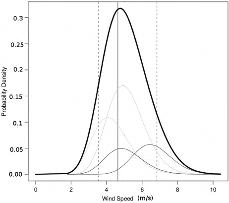
BMA can be understood graphically using Fig. 1, the probabilistic +24 hour wind speed forecast at Johnstown Castle, initialised on the 11 January 2011 at 0000 UTC. Individual forecast ensemble members are represented by the component thin curves. Their variance and weights are found using maximum likelihood estimation on the training data. The weighted component curves are combined to produce the thick curve, the BMA predictive PDF. The dashed vertical lines represent the bounds of the 90% prediction intervals and the verifying observation is represented by the solid vertical line.

Fig. 1.  Example BMA predictive PDF (thick curve) with the component ensemble PDFs (thin curves), the 90% confidence interval bounds (dashed vertical lines) and the verifying observation (thick solid vertical line).

2.3. Selection of the training period

There is no definitive criterion for selecting the length of the training period; a subjective analysis of many factors is required. Here, we investigate how the MAE, CRPS and 60% coverage interval and width vary with different lengths of training period, starting with 10 d and increasing in 5-d intervals to a training period of 60 d. The test period remained fixed, while the training period consisted of the number of training days previous to the test period.

Figure 2 shows how each of the scores varied with the length of the training period for the verification locations, verified over two months. For each experimental training length, the data from the locations is summarised with a boxplot. For each boxplot, the median is represented by the horizontal line, the top and bottom of the box represent the 25th and 75th percentiles, respectively. The whiskers show the maximum and minimum distribution values and the circles represent outliers.

Fig. 2.  MAE, CRPS, coverage and width of 60% confidence interval for different lengths of training periods all stations. MAE, CRPS and width are negatively orientated, and lower scores are better. Coverage is considered best the closer it is to the 60% score.

For MAE and CRPS, there is very little difference amongst the training lengths. The coverage increases with increasing training length, reaching its optimal value of 60% around 55 d. The width values show very little difference with increasing forecast lengths after about 20 d.

Due to the dynamic nature of the weather and the different characteristic time-scales associated with different weather schemes, there will be no perfect length for the training period. The optimal length of training period is also likely to change depending on what season it is being estimated for. Gneiting et al. (2005) describe the trade-off required in selecting the length of the training period between forecast adaptability in the short-term and reduced statistical variability in the longer term. An educated estimate is required and it was decided to make the length of the training period 25 d across all stations balancing the need for increased accuracy and reduced statistical variability with the adaptability of the system to changing weather patterns.

3. Data

The wind speed forecast data used in this study originate from the ECMWF EPS, consisting of one control forecast and 50 perturbed ensemble members. The data are recorded on 63 model levels and interpolated over a regular latitude/longitude grid of 0.5° resolution covering the domain from 30°N to 60°N and 25°W to 45°E. The data were made available by the COSMO Limited-Area Ensemble Prediction System (CLEPS) group and are recorded every three hours from 1 January 2010 to 28 February 2011. Seven dates are missing from the dataset with no more than three consecutively.

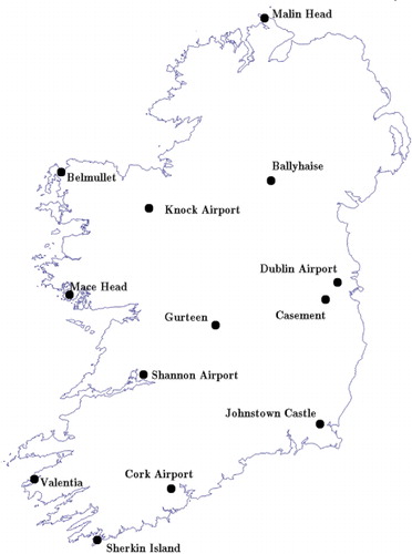
The forecasts are verified at 13 locations around Ireland. The sites correspond to meteorological stations where weather information is recorded hourly and are shown in Fig. 3. The verifying wind speed observations have been provided by Met Éireann in knots and subsequently converted to m s⁻¹.

Fig. 3.  Map of the 13 forecast verification locations used in this study.

Over the time frame of the data, the ensemble mean forecast was found to be more skillful than the individual ensemble members. The MAE of the ensemble mean at +24 hours, averaged across all 13 locations, was 1.701 while the most skillful individual members had an MAE of 1.719. Similarly, at +48 hours the ensemble mean MAE was 1.794, while the individual members could not improve on an MAE of 1.835.

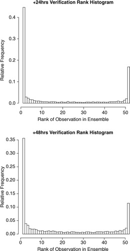
For both forecast intervals, there is a positive relationship between the ensemble range, or the difference between the two ensemble members on either extreme of the distribution, and the absolute forecast error as seen in Fig. 4, the spread-error correlations being 0.27 for +24 hours and 0.48 for +48 hours. However, examination of the verification rank histograms (VRHs) in Fig. 5 show the ensemble to be under-dispersive and hence uncalibrated. As there are 51 ensemble members, it is expected that the observation would be contained within the ensemble range 50 out of 52 times or 96% of the time, but in reality the +24-hour and +48-hour observations were contained only 43% and 59% of the time, respectively. Raftery et al. (2005) explain that this is not an uncommon characteristic of forecast ensembles, which prompted them to develop the BMA technique to produce calibrated and sharp predictive PDFs.

Fig. 4.  Spread-skill relationship for the daily average absolute errors in the +24 hours and +48 hours wind speed forecasts in the ECMWF EPS averaged across all stations for 1 yr. Ensemble range refers to the difference between the two ensembles at either extremes of the distribution. The correlation coefficients were +0.27 and +0.48, respectively.

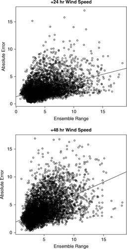
Fig. 5.  Verification rank histograms for the 51 member ECMWF EPS +24 hours and +48 hours wind speed forecasts across all stations using 12 months of data. Both VRHs show spikes at either end of the distribution indicating under-dispersion of the ensemble.

4. Methodology

4.1. Method 1

The first method uses the 51 member ECMWF ensemble as input to the BMA method. The 50 perturbed forecasts differ only in random perturbations. Fraley et al. (2010) describe how constraining these members to be exchangeable deals with their indistinguishability. In practice, this means constraining the weights, variances and bias correction parameters of the exchangeable members to be the same while the control member is considered as a completely separate forecast during the maximum likelihood parameter estimation over the training period.

The BMA method is applied from 21 January 2010 to 26 February 2011, with a 25-d training window. The dates selected will provide consistency of forecast days across both calibration methods with Method 2 requiring longer training. BMA is run separately for each forecast hour from +1 hour to +48 hour and for each station where the ECMWF data are bilinearly interpolated to each location and the wind speed u and v components are converted to ms⁻¹.

4.2. Method 2

The second method involves spatially and temporally downscaling the ECMWF EPS using LAMs. Downscaling all 51 ensemble members would be a computationally expensive exercise, so a clustering algorithm is applied to the members to divide them into eight clusters. Each cluster is assigned a weight based on the number of ensemble members within it. The objective of the clustering method was to find the eight representative members (RMs), one from each cluster, that minimise the within-cluster spread while maximising the between-cluster spread, based on a RMSE distance measure. This is achieved using a clustering method that always selects the ensemble members with the highest and lowest values as two of the RMs. This captures the spread of the under-dispersive ensemble. Selection of the other six RMs could be optimised with alternative clustering methods and this is an area for future research.

Due to the indistinguishability of the ensemble members, there is no consistency between the ensemble members on a day-to-day basis. Consequently, the clustering technique is applied to each forecast day individually and new cluster weights are assigned each day. Clustering is performed on the +48 hour u and v wind speed components at model level 48, the closest level to the 850 mb pressure level where forecasts are not strongly affected by boundary layer disturbances.

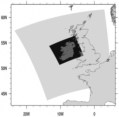
The RM forecasts are downscaled using two LAMs, COSMO (COSMO, 2012) and WRF (Skamarock et al., 2005), at two resolutions. The first domain is of approximately 14 km resolution while the second domain is a nested domain of approximately 3 km resolution. COSMO forecasts are produced using one-way nesting, while WRF forecasts have two-way nesting with feedback from the inner to the outer domain. An outline of the domains can be seen in Fig. 6.

Fig. 6.  Outline of the 14 and 3 km domains used when downscaling the ECMWF representative member forecasts with COSMO and WRF.

The downscaled RM forecasts are produced for every forecast hour from +1 hour to +48 hour and are bilinearly interpolated to the meteorological stations. Each LAM at each resolution produces eight RM downscaled ensemble member forecasts. A weighted ensemble mean forecast is calculated for each downscaled configuration using the respective 8 RM forecasts and their cluster weights. The products of the downscaling process are four weighted ensemble mean forecasts that now exhibit inter-day consistency and can be used as the input to the BMA method. Similar to the ECMWF EPS, the individual ensembles have a mean forecast that is more skillful than the individual ensemble members. They have a positive spread-error correlation and are under-dispersive and therefore uncalibrated. These four weighted ensemble forecast means are used as the input forecasts to the BMA method with the aim of producing a calibrated and sharp predictive PDF. The same dates are used as for Method 1 with no exchangeability constraints.

Raftery et al. (2005) put forward an argument that there may be redundancies of information if the ensemble members are highly correlated. The addition of an ensemble member that is highly correlated with an existing ensemble member will not contribute sufficient information to the BMA method to warrant the additional computational time required to include it.

Table 1 gives the correlation coefficients between the four LAMs weighted ensemble mean forecast errors. The two forecasts derived from the WRF model have a forecast error correlation coefficient of 0.93, which is relatively high due to the two-way nesting of the WRF model that gives feedback from the 3 km domain to the 14 km domain. A decision needs to be made as to whether or not to keep both domains despite this correlation. Figure 7 shows the BMA weights at Johnstown Castle for each of the forecasts over all the forecast days in this study. It is clearly seen that at different times each of the forecasts are assigned the highest weight indicating that, depending on the synoptic situation, each ensemble has more value than the others and therefore none of the forecasts are continually redundant and should be excluded.

Fig. 7.  The BMA weights for the four ensemble member inputs used in Method 2 for Johnstown Castle from February 2010 to February 2011. This shows each of the members contributing significantly to the BMA forecasts at different times during the year and should all be retained for the Method 2 forecast.

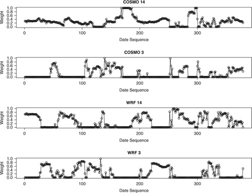
Table 1. Correlation coefficients of the forecasts errors between the four limited area model ensembles based on their weighted ensemble mean forecasts

Ensemble	COSMO 14	COSMO 3	WRF 14	WRF 3
COSMO 14	1	0.59	0.46	0.42
COSMO 3	0.59	1	0.69	0.69
WRF 14	0.46	0.69	1	0.93
WRF 3	0.42	0.69	0.93	1

4.3. Verification techniques

The quality of the forecasts is assessed using a number of well-established techniques. The MAE deterministically assesses the accuracy of a point forecast for each method. The forecasts correspond to the ECMWF ensemble median forecast, the weighted ensemble mean of each of the LAM ensembles and the median of the BMA forecast of each method. The CRPS compares the full distribution with the observation as follows:3

where F(y) is the CDF of the predictand y, and F _o (y) is a step function at the observation where:4 5

The sharper and more accurate the forecast, the closer the CDF is to the step function. This equates to a smaller value under the integral sign in eq. (3), and therefore a lower value of CRPS.

The VRH is a statistical tool to assess the calibration of an ensemble of forecasts. For an ensemble of forecasts to be calibrated, each forecast and the observation can be considered as random samples from the same probability distribution (Hamill, 2001). The ensemble forecasts over a time period are sorted in numerical order. The observation is then ranked relative to the sorted ensemble member forecasts and the frequency of observation rank presented as a histogram. The shape of the VRH gives an indication of its calibration with a flat histogram indicating perfect calibration. The probability integral transform (PIT) histogram is the continuous analogue of the VRH. The CDF value is obtained for each verifying observation and the frequencies ranked and presented as a histogram as before.

The coverage and width of the 90% prediction interval are also used to assess the quality of the forecasts. The coverage refers to the percentage of times the observation falls within the bounds of the 90% prediction interval, with a value close to 90% being considered calibrated. The interval bounds are the wind speeds that correspond to the 0.05 and 0.95 probability forecasts of the PDF and should be as close as possible to indicate a sharp forecast.

5. Results

In this section, we compare the calibration and accuracy of the forecasts using the different calibration methods. Results are given for 2 of the 13 meteorological stations individually as well as the average results across all stations. The two stations were chosen as the ones perceived to give the greatest and least forecast improvements, Johnstown Castle and Knock Airport, respectively, while the station average is considered to be a more representative picture of the results distribution. We start with the results for the original 51 member ECMWF EPS and compare all successive forecasts to this baseline.

5.1. ECMWF data

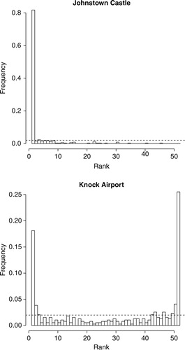
The VRH in Fig. 8 represent the ranks of the observed wind speed value relative to the 51 ensemble member forecasts of the ECMWF. The top VRH represents Johnstown Castle and shows a disproportionately high ranking of the observation below the ensemble range, indicating there may be an over-forecasting bias in the ECMWF data for this station. The bottom VRH representing Knock Airport indicates that the ensemble forecasts at this location are under-dispersive with the verifying observation more often than not falling outside the ensemble range. The dashed lines correspond to the potential height of the bars if the ensemble were calibrated. However, it is clear to see they are not.

Fig. 8.  Example VRHs for Johnstown Castle (top) and Knock Airport estimated using ECMWF EPS data. Ranks are estimated at forecast hours +24 hours for the full year of data. Johnstown Castle shows the observation falling below the ensemble range a large proportion of the time indicating an over-forecasting bias at this station. The Knock Airport histogram shows the observation falling outside the ensemble range on more occasions than within it, indicating under-dispersiveness. The dashed line corresponds to the height of the bars if the ensemble was calibrated

Table 2 shows the MAE, CRPS and coverage and width of the 90% prediction intervals for the same two stations and the average across all stations for all forecast hours. It can be seen that the wind speed forecasts at Knock Airport are distinctly better than those as Johnstown Castle with the average across all stations unsurprisingly somewhere between the two. The lack of coverage at all stations again indicates towards the forecasts being uncalibrated.

Table 2. Accuracy results for the ECMWF ensemble wind speed forecasts

Station	MAE	CRPS	Cov.	Width
Johnstown Castle	2.61	1.98	18	2.02
Knock Airport	0.95	0.72	48	1.60
Average all stations	1.67	1.27	35	1.89

This table consists of the MAE, CRPS and coverage and width of the 90% prediction interval.

5.2. Calibration

5.2.1. Method 1.

The ECMWF 51 member ensemble is used as input to a BMA method as described in section 2. The PIT s for Johnstown Castle and Knock +24 hour wind speed forecasts are displayed in Fig. 9. The PIT histograms indicate that the BMA forecast is a distinct calibration improvement over the original ECMWF EPS data though there is still a small tendency towards an over-forecasting bias for both stations. Post-processing with BMA also appears to have corrected the over-dispersiveness of the ensemble forecasts at Knock Airport.

Fig. 9.  PIT for Johnstown Castle (top) and Knock Airport using ECMWF EPS data post-processed with BMA. The observation is compared to the full predictive PDF. The dashed line corresponds to the height of the bars if the BMA forecast was calibrated. Both PIT histograms display an over-forecasting bias but are an improvement over the uncalibrated ensemble forecast.

5.2.2. Method 2.

Having clustered and downscaled the ECMWF 51 member ensemble to eight RM member forecasts for each LAM, and having calculated a weighted ensemble mean for each LAM, there are four competing forecasts. For each station, the VRH for each LAM showed the general trend of an over-forecasting bias that is evident from the sample VRH s in Fig. 10. Downscaling the model data through the LAMs does not calibrate the forecast.

Fig. 10.  Example VRHs for a LAM forecast for Johnstown Castle (top) and Knock Airport. Ranks are estimated at forecast hours +24 hours for the full year of data. Johnstown Castle shows the observation falling below the ensemble range a large proportion of the time indicating an over-forecasting bias at this station. Knock Airport shows a similar though slightly less extreme pattern. The dashed line corresponds to the height of the bars if the ensemble was calibrated.

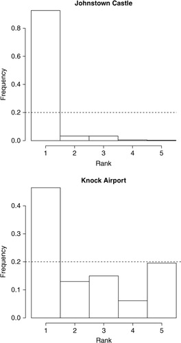
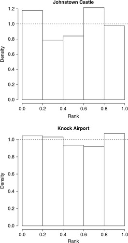
The BMA forecast obtained using the four LAM-weighted ensemble mean forecasts as input, is a more calibrated forecast than the raw forecasts. Evidence of this is seen from the almost flat PIT histograms for Johnstown Castle and Knock Airport +24 hour wind speed forecasts in Fig. 11. The application of both Method 1 and Method 2 to the ECMWF EPS improves the calibration of the forecasts. Close inspection of Figs. 9 and 11 would indicate that both methods induce a similar level of calibration on the forecasts. The figures shown here are representative of the calibration patterns obtained for each of the 13 meteorological stations. We now compare the accuracy of the two methods to establish which method produces the greatest forecast improvements.

Fig. 11.  PIT for Johnstown Castle (top) and Knock Airport LAM ensemble forecasts combined and post-processed with BMA. The observation is compared to the full predictive PDF. The dashed line corresponds to the height of the bars if the BMA forecast was calibrated. Both PIT histograms show good calibration.

5.3. Accuracy

The accuracy of the two calibration methods is detailed in Tables 3–5 in terms of the MAE, CRPS and coverage and width of the 90% prediction interval and correspond to the Johnstown Castle, Knock Airport and average station forecasts, respectively. The average ensemble forecast results and the BMA forecast results are detailed for both BMA methods and the original ECMWF results are reiterated for comparative purposes.

Table 3. Numerical results for ECMWF ensemble forecast and the two calibration methods for Johnstown Castle

Forecast	MAE	CRPS	Cov.	Width
ECMWF	2.61	1.98	18	2.02
Method 1 – Avg Ens	2.61	2.25	88	2.24
Method 1 – BMA	0.90	0.63	63	3.53
Method 2 – Avg Ens	2.62	2.42	31	5.08
Method 2 – BMA	0.87	0.62	84	3.28

Coverage and width refer to the 90% prediction interval. The best results are displayed in bold font for clarity.

The numerical results for Johnstown Castle in Table 3 show that the Method 2 BMA forecast is the most accurate as both a deterministic and probabilistic forecast with the lowest MAE and CRPS and considerable improvements over the original ECMWF ensemble forecasts. The coverage of the 90% prediction interval is also good. The trade-off in using this method is that it widens the 90% prediction interval. However, the forecast has become more calibrated. Both BMA methods have evident accuracy improvements over their respective average ensemble forecasts.

Knock Airport (Table 4) had a very good original ECMWF ensemble forecast for wind speeds and improving on these numerical accuracy results proved difficult. The first BMA method made the forecasts slightly less accurate while the second BMA method made a marginal improvement to the CRPS while worsening the deterministic MAE score. These disimprovements are small in comparison to the improvements made to the calibration of the wind speed forecast at Knock Airport so overall it can be argued that post-processing the LAM forecasts with BMA does add value to the forecasts at this location. As Knock Airport showed the least improvement in accuracy of all 13 stations using the BMA method, it can be derived that at every station value is added to the wind speed forecast by statistically post-processing them in this way. This result is mirrored in Table 5 which shows the accuracy results averaged across all 13 stations. At an individual station level, there was no correlation between the accuracy of the forecasts and the location around Ireland or proximity to the coast. Overall, improvements can be made to the forecasts, assessed both deterministically and probabilistically, by post-processing each method with BMA. As we have previously shown, applying the BMA method also improves the calibration.

Table 4. Numerical results for ECMWF ensemble forecast and the two calibration methods for Knock Airport

Forecast	MAE	CRPS	Cov.	Width
ECMWF	0.95	0.72	47	1.60
Method 1 – Avg Ens	0.97	0.75	88	1.80
Method 1 – BMA	1.01	0.72	85	3.89
Method 2 – Avg Ens	1.12	0.92	73	3.35
Method 2 – BMA	0.98	0.70	84	3.68

Coverage and width refer to the 90% prediction interval. The best results are displayed in bold font for clarity.

Table 5. Numerical results for ECMWF ensemble forecast and the two calibration methods averaged over all stations

Forecast	MAE	CRPS	Cov.	Width
ECMWF	1.67	1.27	35	1.89
Method 1 – Avg Ens	1.67	1.40	88	2.12
Method 1 – BMA	1.23	0.89	86	4.98
Method 2 – Avg Ens	1.54	1.29	69	4.94
Method 2 – BMA	1.18	0.85	85	4.68

Coverage and width refer to the 90% prediction interval. The best results are displayed in bold font for clarity.

By taking the ECMWF 51 member ensemble, clustering it to eight RMs, downscaling the RMs through four LAMs and calculating a weighted ensemble mean forecast, then using these forecasts as input to a BMA procedure, the forecasts transform from being under-dispersive to being calibrated and more accurate. The MAE and CRPS scores improve by 29% and 33%, respectively, averaged across all 13 stations over a full year. Though the results shown here were for the +24 hour wind speed forecasts, very similar trends were seen in both calibration and accuracy across forecast hours +1 to +48 hours.

6. Conclusions

The ECMWF produces an EPS that despite showing a positive spread-error correlation, is under-dispersive and therefore uncalibrated. We have put forward two methods of post-processing the ECMWF EPS with the aim of producing a more calibrated and accurate probabilistic forecast for the wind energy industry. Both methods use BMA, with a fixed training period of 25 d to calibrate the forecasts with varying degrees of success. Method 1 involves constraining the 50 perturbed ensemble members to be equal which increased the calibration and accuracy of the forecast. Method 2 produced forecasts with similar calibration to those produced by Method 1. However, they were the best forecasts in terms of accuracy and thus added the most value to the wind speed forecasts in terms of the end users in the wind energy industry. This method clustered and downscaled the ECMWF data through four LAMs which were then used, in conjunction with the cluster weights, to produce a weighted ensemble mean forecast for each LAM. These forecasts were used as input to the BMA method. The methods were applied to forecast lead times of +1 hour to +48 hour indicating that probabilistic forecast improvements have been made to wind speed forecasts in the short to medium-term time frame across all verification locations.

7. Acknowledgments

This study is based upon work supported by the Science Foundation of Ireland (SFI) under Grant no. 09/RFP/MTH2359. The authors wish to acknowledge the Irish Centre for High-End Computing (ICHEC) for the provision of computational facilities and support, Met Éireann for kindly supplying the observed wind speed data, the COSMO Limited-Area Ensemble Prediction System (CLEPS) group for supplying the ECMWF EPS data, and Prof. Adrian Raftery of the University of Washington for his expertise and guidance in the area of BMA. Finally, we are grateful to two anonymous reviewers who offered helpful comments and suggestions.

References

- Arribas A. Robertson K. B. Mylne K. R. Test of a poor man's ensemble prediction system for short-range probability forecasting. Mon. Weather Rev. 2005; 133: 1825–1839. 10.3402/tellusa.v65i0.19669.
- Candille G. Talagrand O. Evaluation of probabilistic prediction systems for a scalar variable. Q. J. Roy. Meteorol. Soc. 2005; 131: 2131–2150. 10.3402/tellusa.v65i0.19669.
- Celik A. N. A statistical analysis of wind power density based on the Weibull and Rayleigh models at the southern region of Turkey. Renew. Energ. 2004; 29: 593–604. 10.3402/tellusa.v65i0.19669.
- Chmielecki R. M. Raftery A. E. Probabilistic visibility forecasting using Bayesian model averaging. Mon. Weather Rev. 2011; 139: 1626–1636. 10.3402/tellusa.v65i0.19669.
- COSMO. 2012. COSMO public area. The Consortium for Small-scale Modeling (COSMO). Online at: http://cosmo-model.org.
- Fraley C. Raftery A. E. Gneiting T. Calibrating multimodel forecast ensembles with exchangeable and missing members using Bayesian model averaging. Mon. Weather Rev. 2010; 138: 190–202. 10.3402/tellusa.v65i0.19669.
- Garcia A. Torres J. de Francisco A. Fitting wind speed distributions: a case study. Sol. Energ. 1998; 62: 139–144. 10.3402/tellusa.v65i0.19669.
- Garcia-Moya J.-A. Callado A. Escriba P. Santos C. Santos-Munoz D. Simarro J. Predictability of short-range forecasting: a multimodel approach. Tellus A. 2011; 63: 550–563. 10.3402/tellusa.v65i0.19669.
- Gneiting T. Balabdaoui F. Raftery A. E. Probabilistic forecasts, calibration and sharpness. J. Roy. Stat. Soc B. 2007; 69: 243–268. 10.3402/tellusa.v65i0.19669.
- Gneiting T. Raftery A. E. Westveld A. H. Goldman T. Calibrated probabilistic forecasting using ensemble model output statistics and minimum CRPS estimation. Mon. Weather Rev. 2005; 133: 1098–1118. 10.3402/tellusa.v65i0.19669.
- Hamill T. M. Interpretation of rank histograms for verifying ensemble forecasts. Mon. Weather Rev. 2001; 129: 550–560.
- Johnson C. Swinbank R. Medium-range multimodel ensemble combination and calibration. Q. J. Roy. Meteorol. Soc. 2009; 135: 777–794. 10.3402/tellusa.v65i0.19669.
- Jolliffe, I. T and Stephenson, D. B. 2011. Forecast Verification: A Practitioners Guide in Atmospheric Science. 2nd ed. Wiley-Blackwell: Chichester, p. 248.
- Leutbecher M. Palmer T. Ensemble forecasting. J. Comput. Phys. 2008; 227: 3515–3539. 10.3402/tellusa.v65i0.19669.
- Marrocu M. Chessa P. A. A multi-model/multi-analysis limited area ensemble: calibration issues. Meteorol. Appl. 2008; 15: 171–179. 10.3402/tellusa.v65i0.19669.
- Murphy A. H. What is a good forecast? An essay on the nature of goodness in weather forecasting. Weather Forecast. 1993; 8: 281–293.
- Nipen T. Stull R. Calibrating probabilistic forecasts from an NWP ensemble. Tellus A. 2011; 63: 858–875. 10.3402/tellusa.v65i0.19669.
- Raftery A. E. Gneiting T. Balabdaoui F. Polakowski M. Using Bayesian model averaging to calibrate forecast ensembles. Mon. Weather Rev. 2005; 133: 1155–1174. 10.3402/tellusa.v65i0.19669.
- Roulston M. S. Smith L. A. Combining dynamical and statistical ensembles. Tellus A. 2003; 55: 16–30. 10.3402/tellusa.v65i0.19669.
- Silva, E. 2007. Analysis of the characteristic features of the density functions for gamma, Weibull and log-normal distributions through RBF network pruning with QLP. Proc. 6th WSEAS Int. 223–228.
- Skamarock, W, Klemp, J., and Dudhia, J. 2005. A Description of the Advanced Research WRF Version 2. NCAR Tech. Notes-468 + STR.
- Sloughter J. M. Gneiting T. Raftery A. E. Probabilistic wind speed forecasting using ensembles and Bayesian model averaging. J. Am. Stat. Assoc. 2010; 105: 25–35. 10.3402/tellusa.v65i0.19669.
- Sloughter J. M. Raftery A. E. Gneiting T. Fraley C. Probabilistic quantitative precipitation forecasting using Bayesian model averaging. Mon. Weather Rev. 2007; 135: 3209–3220. 10.3402/tellusa.v65i0.19669.
- Soman, S, Zareipour, H, Member, S, Malik, O., and Fellow, L. 2005. A review of wind power and wind speed forecasting methods with different time horizons. In: North American Power Symposium (NAPS). 2010. Arlington, Texas, Vol. 4, pp. 1–8.
- Sweeney C. Lynch P. Adaptive post-processing of short-term wind forecasts for energy applications. Wind Energy. 2011; 14: 317–325. 10.3402/tellusa.v65i0.19669.
- Sweeney, C, Lynch, P., and Nolan, P. 2011. Reducing errors of wind speed forecasts by an optimal combination of post-processing methods. Meteorol Appl. DOI: 10.3402/tellusa.v65i0.19669.
- Thorarinsdottir T. L. Gneiting T. Probabilistic forecasts of wind speed: ensemble model output statistics by using heteroscedastic censored regression. J. Roy. Stat. Soc. A (Statistics in Society). 2010; 173: 371–388. 10.3402/tellusa.v65i0.19669.
- Tian X. Xie Z. Wang A. Yang X. A new approach for Bayesian model averaging. Science China Earth Sci. 2012; 55: 1336–1344. 10.3402/tellusa.v65i0.19669.
- Unger D. A. van den Dool H. O'Lenic E. Collins D. Ensemble regression. Mon. Weather Rev. 2009; 137: 2365–2379. 10.3402/tellusa.v65i0.19669.
- Wilks D. S. Smoothing forecast ensembles with fitted probability distributions. Q. J. Roy. Meteorol. Soc. 2002; 128: 2821–2836. 10.3402/tellusa.v65i0.19669.