Radar radial wind data assimilation using the time-incremental 4D-Var method implemented to the WRFDA system

Abstract

In this study, we selected a heavy rainfall case over the Korean Peninsula, which was characterised by two localised rainfall maxima. Neither of the two maxima is accurately simulated when no radar data are assimilated or when radar data are assimilated using the three-dimensional variational (3D-Var) method of the Weather Research and Forecasting Data Assimilation (WRFDA) system. Using the four-dimensional variational (4D-Var) method included in the WRFDA system improves the rainfall forecast partially. To obtain further improvements in the rainfall forecast, outer loops and the time-incremental 4D-Var method are used. In the time-incremental 4D-Var method, the length of the assimilation window is increased gradually, and the starting point of the current minimisation task comes from the minimiser of the previous minimisation task. The analysis of the experiment using outer loops or the time-incremental 4D-Var method is closer to the observations than that of the experiment using the 4D-Var method. This is because the first guess is improved progressively by using outer loops or the time-incremental 4D-Var method. The gap between nonlinear and linear growth is reduced via outer loops or the time-incremental 4D-Var method compared to the 4D-Var method, because the nonlinearity is accounted for by consistently updating the nonlinear model trajectory. However, the rainfall forecast is improved only in the experiment using the time-incremental 4D-Var method. Analysis increments of the horizontal wind and convective available potential energy (CAPE) result in proper modifications to the analysis, and finally, an improved subsequent forecast. The quasi-static adjustment in the time-incremental 4D-Var method may contribute to finding the global minimum under the high degree of nonlinearity present in the original minimisation problem.

• time-incremental 4D-Var method
• outer loop
• nonlinearity
• heavy rainfall
• radar data assimilation

1. Introduction

Data assimilation can be defined as the process through which all the available information is used to estimate the state of the atmospheric flow as accurately as possible (Talagrand, 1997). Data assimilation methods can be divided into two groups: sequential methods and variational methods. Sequential methods are based on the minimum-variance approach, and examples are the optimal interpolation (OI; Gandin, 1963), extended Kalman filter (EKF) and ensemble Kalman filter (EnKF; Evensen, 1994) methods. Variational methods are based on the maximum-likelihood approach, and examples are the three-dimensional variational (3D-Var) and four-dimensional variational (4D-Var; Lewis and Derber, 1985; Le Dimet and Talagrand, 1986) methods. 4D-Var is a very sophisticated method implemented in several operational centres including the European Centre for Medium-Range Weather Forecasts (ECMWF; Rabier et al., 2000), Météo-France (Gauthier and Thépaut, 2001), the Met Office (Rawlins et al., 2007), the Japan Meteorological Agency (JMA; Honda et al., 2005), Environment Canada (Gauthier et al., 2007), the High-Resolution Limited-Area Model (HIRLAM; Huang et al., 2002), and the Naval Research Laboratory Atmospheric Variational Data Assimilation System (NAVDAS-AR; Xu et al., 2005).

Radar data assimilation is essential for extending the predictability of numerical weather prediction (NWP), especially when high-resolution simulation is considered. Xiao et al. (2005) assimilated Doppler radar radial velocity data using the fifth-generation Pennsylvania State University/National Center for Atmospheric Research Mesoscale Model (MM5) and its 3D-Var system. The observation operator for Doppler radial velocity was developed, and the dynamic balance based on the Richardson equation was introduced to assimilate Doppler radial velocity observations. In Xiao et al. (2007), the observation operator for radar reflectivity was developed, and total water mixing ratio was used as a control variable within the MM5 3D-Var system to assimilate radar reflectivity data. Additionally, a warm-rain process was incorporated into the system to partition the moisture and hydrometeor increments. Recently, the MM5 model and its 3D-Var system were upgraded to the Weather Research and Forecasting (WRF) model and its 3D-Var system. The impact of multiple Doppler radar data assimilation on Quantitative Precipitation Forecasting (QPF) of a squall line was investigated (Xiao and Sun, 2007), and results of operational Doppler radar data assimilation in the Korean Meteorological Administration (KMA) were reported (Xiao et al., 2008b) using the WRF 3D-Var system. Wang et al. (2013) developed the WRF 4D-Var radar data assimilation system including tangent linear and adjoint models of a Kessler warm-rain microphysics scheme and new control variables of cloud water, rain water and vertical velocity. The newly developed WRF 4D-Var radar data assimilation system was compared with the corresponding WRF 3D-Var system for a squall line case over the US Great Plains. Sun and Crook (1997, 1998) assimilated Doppler radial velocity and reflectivity data into a cloud-scale model using the Variational Doppler Radar Analysis System (VDRAS). The VDRAS was also implemented in Beijing, China, and contributed to the Beijing 2008 Forecast Demonstration Project in support of the Beijing Summer Olympics (Sun et al., 2010). Based on the previous studies, it can be concluded that to use 4D-Var is essential for assimilating high-resolution radar data more efficiently.

Generally, 4D-Var is implemented using an incremental formulation, which approximates the minimisation of the nonlinear cost function by a sequence of minimisations of linear least-squares cost functions (Courtier et al., 1994; Haben et al., 2011). The incremental formulation has the advantage of allowing further approximations in the solution procedure, such as lower resolution inner loop and simplified tangent linear and adjoint models, to make the minimisation problem computationally feasible. In the incremental formulation, the linearised cost function is minimised in an inner loop, and the nonlinear model trajectory, which is used for linearisation of the nonlinear model and observation operator, and first guess are updated in an outer loop. Nonlinearities related to the model and the observation operator can be taken into account in the outer loop because the nonlinear model trajectory for linearisation is consistently updated. The quality of the analysis can be improved and more observations can be utilised by using more than one outer loops (Rizvi et al., 2008).

Pires et al. (1996) investigated how the accuracy of the state obtained at the end of the assimilation window varies when the length of the assimilation window is theoretically increased back to infinity using the three-variable system introduced by Lorenz (1963) under the assumption of a perfect model. In the limit of infinitely long assimilation periods, the chaotic nature of the system produces a number of local minima. The quasi-static variational assimilation (QSVA) algorithm was proposed to determine the global minimum and to avoid getting trapped near a local minimum, and it is based on successive small increments of the assimilation window and quasi-static adjustments of the minimising solution. The algorithm was also applied to a quasi-geostrophic model, and it was effective in solving the minimisation problem with the assimilation window of the order of 5–10 d.

The computational cost is usually concentrated just after the so-called cut-off time, that is, after the end of the assimilation period. Järvinen et al. (1996) proposed an alternative implementation of 4D-Var, the quasi-continuous variational assimilation approach (similar to the QSVA algorithm; hereafter, the term ‘time-incremental 4D-Var’ is used instead of the QSVA or quasi-continuous variational assimilation), to reduce the peak computational requirements of 4D-Var after the cut-off time and to accelerate the convergence of the minimisation of the cost function. The feasibility of the approach was first validated with a low-resolution barotropic grid-point model using synthetic observations, and the results were then confirmed with a multi-level primitive equation model using real observations.

In this study, we assimilate radar radial velocity data for a heavy rainfall case over the Korean Peninsula using the Weather Research and Forecasting Data Assimilation (WRFDA) system (Huang et al., 2009). The WRFDA system includes 3D-Var and 4D-Var capabilities, and the outer loop can be used within the 4D-Var capability. We implement the time-incremental 4D-Var algorithm into the WRF 4D-Var, and compare it with single outer-loop 4D-Var and multiple outer-loop 4D-Var. Despite the usefulness of the outer loop, there have been few studies on its effect. The purpose of this study is to compare the time-incremental 4D-Var method with the 4D-Var and outer-loop methods, focusing on the quality of the first guess and the nonlinearity of the minimisation problem. We also investigate analysis increments to figure out the reason for forecast differences. Finally, we suggest a strategy for the implementation of the time-incremental 4D-Var method in an operational environment.

This article is laid out as follows. In Section 2, the theoretical background on the time-incremental 4D-Var algorithm is summarised. Section 3 includes the experimental design and a description of the case. The results and corresponding discussion are presented in Section 4. Finally, Section 5 contains a summary and conclusions.

2. The time-incremental 4D-Var algorithm

In the 4D-Var method, the cost function is a measure of the weighted sum of squared distances to the background and to the observations distributed over the assimilation window, and it is minimised to find the analysis.1 where x ₀ is a control variable of the above minimisation problem, the subscript 0 denotes the time t=t ₀, is the background state defined at t=t ₀, and B ₀ is the background error covariance also defined at t=t ₀. is the observations at t=t _n , the subscript n varies from 0 to N, and R _n is the observation error covariance. H _n is the nonlinear observation operator and M _n is the nonlinear model operator, which evolves over time from x ₀ to x _n valid at t=t _n .

When an analysis increment is defined as the difference between x ₀ and the first guess, the cost function can be rewritten, after some manipulation, as follows. 2 where δx ₀ is the analysis increment, is the first guess defined at t=t ₀, and d _n is the innovation. H _n and M _n are the linearised observation and model operators, respectively.

In the time-incremental 4D-Var algorithm, the time interval of an assimilation window is gradually increased from [t ₀,t ₀] to [t ₀,t _N ]. If we define the cost function of 4D-Var with simplified notation,3 the cost function for each step of the time-incremental 4D-Var algorithm can be written as follows.4 where A _n is the nth minimisation task of the time-incremental 4D-Var algorithm. It is noted that for the nth minimisation task, A _n , the starting point for the minimisation of the cost function comes from the minimiser of the previous minimisation task, A _n−1. In other words, in the time-incremental 4D-Var algorithm, the first guess, not the background, is updated, and hence there is no correlation between background and observation errors.

3. Experimental design and case description

3.1. Experimental design

In this study, we used the Advanced Research Weather Research and Forecasting (ARW-WRF) model (Skamarock et al., 2008) as a forecasting model. A total of six experiments are carried out, and details of the experiments are given in Table 1. Triply-nested domains, focusing on South Korea, with horizontal resolutions of 54 km (domain 1), 18 km (domain 2) and 6 km (domain 3) are employed (Fig. 1). The number of horizontal grid points for each domain is 120×102, 121×103 and 121×127, respectively, and the number of vertical levels for all of the domains is 35 with the model top at 50 hPa. The selected physics schemes for nonlinear-model runs are the WRF Single-Moment 6-class (WSM6) with graupel microphysics scheme (Hong and Lim, 2006), the Kain–Fritsch cumulus parameterization scheme (Kain, 2004), the Yonsei University (YSU) planetary boundary layer scheme (Hong et al., 2006), the Rapid Radiative Transfer Model (RRTM) longwave radiation scheme (Mlawer et al., 1997) and the Dudhia shortwave radiation scheme (Dudhia, 1989). The simplified physics schemes are employed for tangent linear- and adjoint-model runs: surface friction, cumulus parameterisation and large-scale condensation (Zhang et al., 2013). These schemes are similar to the physics packages used in the WRF Adjoint Modeling System (WAMS; Xiao et al., 2008a). The global final analysis (FNL) data from the National Center for Environmental Prediction (NCEP) with a horizontal resolution of approximately 100 km are used to create initial and boundary conditions. Initial time for domain 1, domain 2 and domain 3 is 1200 UTC, 5, 0000 UTC, 6 and 0600 UTC, 6 August 2006, respectively, and only the 6-h forecast of domain 3 is considered for validation here.

Fig. 1 Domain configuration. (a) Geographical area for domains 1, 2 and 3 and (b) model terrain height (m) for domain 3. Locations of Namwon, Taebaek and Gwangju cities are also indicated.

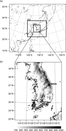
Table 1 Brief description for each numerical experiment

Experiment name	Description
CONTROL	No radar data are assimilated
3DVAR	Radar data are assimilated using the 3D-Var method
4DVAR	Radar data are assimilated using the 4D-Var method (with single outer loop)
OUTER	Radar data are assimilated using the 4D-Var method with 3 outer loops
QSVA	Radar data are assimilated using the time-incremental 4D-Var method
QSVA_LC	Same as QSVA experiment except for loose inner-loop stopping criterion

The WRFDA system version 3.4 (Huang et al., 2009) is used for all the data assimilation experiments, and the data assimilation experiments are conducted only on domain 3. The WRFDA system has both 3D-Var and 4D-Var (and outer loop) capabilities and the time-incremental 4D-Var algorithm introduced in Section 2 is implemented. Although simplified physics schemes are used in the inner-loop minimisation, the same resolution as the nonlinear-model run is used in the minimisation. Background for all the data assimilation experiments is the initial condition of the CONTROL experiment (i.e. cold start), and the 6-h forecast from 0600 UTC to 1200 UTC, 6 August 2006 is made using the analysis of each data assimilation experiment. The background error covariance is calculated using the National Meteorological Center (NMC) method (Parrish and Derber, 1992), in which the background error statistics are derived from the differences between 24- and 12-h forecasts for the 1-month period of August 2006.

Radar data from 13 radar observation sites over the Korean Peninsula are assimilated in this study. Only radar radial velocity data are assimilated although measured quantities are radial velocity, reflectivity and spectrum width. A detailed description of the radar data over the Korean Peninsula can be found in Park and Lee (2009). In advance of being assimilated, radar data are pre-processed using the methods given by Park and Lee (2009). The pre-processing includes quality control, interpolation/thinning to Cartesian grids by the Sorted Position Radar INTerpolation (SPRINT; Mohr and Vaughan, 1979; Miller et al., 1986) and Custom Editing and Display of Reduced Information in Cartesian coordinate (CEDRIC; Mohr et al., 1986) packages and hole-filling/smoothing by the CEDRIC package. The details of the quality control are as follow. The on-site signal processors of the individual radars first process noises and errors embedded in the radar data. Mapping the radar measurements onto the Digital Elevation Model (DEM) data eliminates the remaining ground clutters. The anomalous echoes are removed manually using radar images. Furthermore, the aliasing effect of the radial velocity measurements is corrected based on a spatial continuity constraint along the radial and azimuth directions. The speckling due to the dual-pulse repetition frequency (PRF) velocity error is removed by a simple elimination technique. The radar data have a horizontal resolution of approximately 6 km and a vertical resolution of about 0.5 km. For the observation error covariances, only variances are considered (i.e. observation error covariance matrix is diagonal), and the assumed observational error of radial velocity is 2 m s⁻¹. The assimilation window covers the period from 0600 UTC to 0630 UTC, 6 August 2006, and radar data are provided every 10 minutes within the assimilation window. The observation operator for radar radial velocity developed by Xiao et al. [2005; Eqs. (3)–(5) of their study] is used in this study.

3.2. Case description

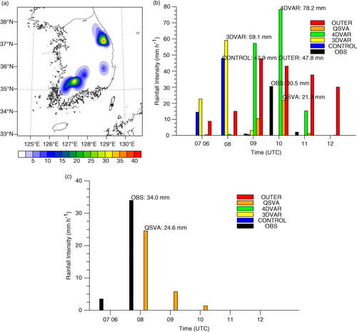
The heavy rainfall case for this study can be categorised as an air-mass thunderstorm that developed as a result of daytime solar heating. Figure 2 shows the 6 h accumulated rainfall distribution over South Korea and the time series of hourly rainfall at the two localised rainfall maxima (Taebaek and Namwon; refer to Fig. 1b) for the period of 0600 UTC to 1200 UTC, 6 August 2006. The rainfall distribution was processed by the smoother introduced in Haltiner and Williams [1980; their Eq. 11.107] to represent its characteristics more clearly. Rainfall was concentrated over the east coast and the southwestern part of the Korean Peninsula. Over the east coast, hourly rainfall at the maximum peaked at 0800 UTC, 6 August 2006 and the 6 h accumulated rainfall was 37.5 mm. Over the southwestern part, the 6 h accumulated rainfall at the maximum was 33.5 mm and it peaked at 1000 UTC, 6 August 2006. Note that rainfall was localised over a small area and it was concentrated near the peak time.

Fig. 2 (a) Observed 6 hours accumulated rainfall (mm 6 h⁻¹) distribution over South Korea from 0600 UTC to 1200 UTC, 6 August 2006. Time series of hourly rainfall (mm h⁻¹) from 0600 UTC to 1200 UTC, 6 August 2006 for the observations (black), CONTROL (blue), 3DVAR (yellow), 4DVAR (green), QSVA (orange) and OUTER (red) experiments at (b) Namwon and (c) Taebaek. Rainfall observations are from the Korea Meteorological Administration (KMA) surface observations. In the case of numerical experiments, hourly rainfalls at the grid points corresponding to Namwon and Taebaek are shown.

In this case, the atmosphere over the Korean Peninsula was unstable because the Korean Peninsula was located along the edge of a North Pacific high-pressure system. Warm and moist air was transported to the Korean Peninsula along the edge of the North Pacific high at the 850 hPa level. In contrast, cold air surged into the Korean Peninsula by a northwesterly flow related to a cold trough at the 200 hPa level (figures not shown). This synoptic environment caused the atmosphere over the Korean Peninsula to be conditionally unstable. The thermodynamic quantities obtained by analysing the skew T-log p diagrams of Gwangju, one of radiosonde stations in South Korea, which is approximately 50 km southwest of the southwestern maximum (refer to Fig. 1b), are given in Table 2. Cold air was supplied continuously at upper levels by an upper-level trough, and after sunrise, the land surface was heated by solar heating. This destabilised the atmosphere and raised convective available potential energy (CAPE) and lowered convective inhibition (CIN). During the same period, the level of free convection (LFC) was lowered.

Table 2 Convective available potential energy (CAPE, J kg⁻¹), convective inhibition (CIN, J kg⁻¹), lifting condensation level (LCL, m) and level of free convection (LFC, m) computed from sounding observations of Gwangju at 0000 UTC and 0600 UTC, 6 August 2006

	CAPE	CIN	LCL	LFC
0000 UTC, 6 August 2006	124	217	451	3836
0600 UTC, 6 August 2006	1970	6	1152	1456

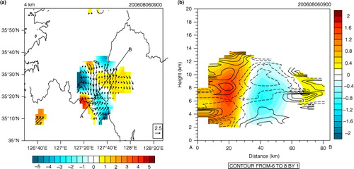
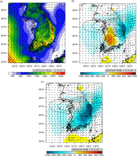
Figure 3 shows the horizontal cross section of the horizontal wind and divergence at a height of 4 km and the vertical cross section of the vertical wind and divergence along the line in the horizontal cross section. At the southwestern maximum, the hourly rainfall from 0900 UTC to 1000 UTC, 6 August 2006 was greatest, and therefore the cross sections for 0900 UTC are shown. For these radar data-based analyses, three-dimensional wind fields are retrieved and synthesised using radar radial velocity data over the Korean Peninsula. As previously mentioned, the atmosphere over the southwestern part of the Korean Peninsula was conditionally unstable. In other words, if there is a forcing for lifting of the air parcel to its LFC, a strong upward motion and (if there is enough moisture) a large amount of rainfall can be induced. A northerly or northwesterly flow and a southwesterly flow met near the southwestern maximum, and this formed a convergence zone (Fig. 3a). This convergence acted as a lifting forcing, and there was torrential rainfall, lasting approximately 1 hour from 0900 UTC. The updraft related to the convective instability extended to near the tropopause with a maximum value of approximately 2 m s⁻¹ at a height of 7 km. There was also a compensating downdraft beside the updraft, which was related to upper-level convergence and lower-level divergence (Fig. 3b).

Fig. 3 Radar analyses near Namwon area at 0900 UTC, 6 August 2006. (a) Horizontal distribution of divergence (10⁻⁴ s⁻¹, shading) and winds (m s⁻¹, vector) at 4-km height. (b) Vertical cross section along the line shown in (a) of vertical wind (m s⁻¹, shading) and divergence (10⁻⁴ s⁻¹, negative values are denoted by dashed contours).

4. Results and discussion

4.1. Data assimilation results

Table 3 shows values of the cost function at the first and last iterations and total number of iterations for data assimilation experiments. The conjugate gradient method is used to solve a linearised minimization problem, and the minimisation is terminated when the gradient norm decreases by two orders of magnitude, as suggested by Daley and Barker (2001). In the 3DVAR and 4DVAR experiments, the minimisation converges after several iterations. Originally, a total of four outer loops are used in the OUTER experiment, and inner-loop minimisation for each outer loop successfully converges. There is a divergence at the fourth outer loop, and hence the OUTER experiment refers to the use of the 4D-Var method with three outer loops. In the QSVA experiment, the minimisation for each assimilation window converges after several iterations. It should be noted that the ending value of the cost function in the QSVA experiment is less than that in the 4DVAR experiment, and it is similar to that in the OUTER experiment.

Table 3 Cost-function values at the first and last iterations and total number of iterations for the 3DVAR, 4DVAR, OUTER and QSVA experiments

	3DVAR	4DVAR	OUTER (2)	OUTER (3)	OUTER (4)	QSVA (0)	QSVA (10)	QSVA (20)	QSVA (30)
Initial cost-function value	1735.87	7877.05	3789.28	3643.60	3619.12	1735.87	1971.65	2961.01	3821.68
Final cost-function value	976.95	3640.80	3597.56	3561.16	3565.03	976.95	1788.47	2796.00	3563.56
Total number of iterations	12	21	26	26	29	12	20	22	25

The number in parenthesis in the OUTER experiment indicates the number of outer loops applied and that in the QSVA experiment indicates the length of the assimilation window (in minute) for each assimilation task.

Table 4 shows the root mean square errors (RMSEs) of O−B (observation minus background) or O−FG (observation minus first guess) and O−A (observation minus analysis) for zonal wind, meridional wind and radial velocity. To calculate the RMSEs for zonal and meridional winds (radial velocity), radiosonde (radar radial velocity) observations over the Korean Peninsula are used. It is noted that only radar radial velocity data are assimilated, and hence radiosonde observations are independent. The number of assimilated radial velocity observations is also shown. In all of the data assimilation experiments, the RMSE of O−A is smaller than that of O−B or O−FG, which is a natural result of data assimilation. In the 4DVAR experiment, the RMSEs of O−B and O−A for zonal (meridional) wind are 1.625 (2.498) and 1.533 (2.336), respectively. As the number of applied outer loops is increased, the RMSE of O−A is consistently reduced in the OUTER experiment. Similarly, the RMSE of O−A is continuously decreased with the increasing length of the assimilation window in the QSVA experiment in spite of the increase in the number of assimilated observations. As a result, the RMSE of O−A for the OUTER or QSVA experiment is smaller than that for the 4DVAR experiment, and this is due to the improved first guess in the OUTER or QSVA experiment. The O−B (O−FG)/O−A statistics for radial velocity are consistent with those for zonal and meridional winds. The number of assimilated observations in the OUTER and QSVA experiments is greater than that in the 4DVAR experiment although the difference is not significant.

Table 4 Root mean square errors (RMSEs, m s⁻¹) of O−B (or O−FG) and O−A for zonal wind, meridional wind and radial velocity using radiosonde and radar observations over the Korean Peninsula for the 3DVAR, 4DVAR, OUTER and QSVA experiments

	3DVAR	4DVAR	OUTER (2)	OUTER (3)	QSVA (0)	QSVA (10)	QSVA (20)	QSVA (30)
U
O−B	1.625	1.625	1.533	1.526	1.625	1.616	1.589	1.523
O−A	1.616	1.533	1.526	1.522	1.616	1.589	1.523	1.514
V
O−B	2.498	2.498	2.336	2.333	2.498	2.441	2.404	2.334
O−A	2.441	2.336	2.333	2.328	2.441	2.404	2.334	2.308
Rv
O−B	2.272	2.270	1.479	1.441	2.272	1.616	1.545	1.508
O−A	1.603	1.446	1.431	1.417	1.603	1.479	1.465	1.424
Number of assimilated OBSs	2691	12 226	12 228	12 228	2691	5694	9142	12 228

The number of assimilated radar radial velocity observations is also shown. The number in parenthesis in the OUTER experiment indicates the number of outer loops applied and that in the QSVA experiment indicates the length of the assimilation window (in minute) for each assimilation task.

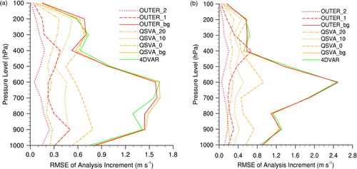
Vertical distribution of the root mean square difference between the analysis and background or first guess (RMSD of analysis increment) for the 4DVAR, OUTER and QSVA experiments are shown in Fig. 4. For the OUTER experiment, analysis increments are calculated by using the analysis and the original first guess or updated first guesses from the analyses of the first and second outer loops. Similarly, for the QSVA experiment, the original first guess or updated first guesses from the analyses of assimilation tasks with 0-, 10- and 20-minute assimilation window is used when analysis increments are calculated. In the 4DVAR experiment, analysis increments of both zonal and meridional wind are the largest at about 600 hPa, where radial velocity data are plentiful. In other words, analysis increments between 700 and 400 hPa (i.e. mid-levels) are large because more observations are assimilated at those levels. Analysis increments at lower or upper levels, where radial velocity data are relatively scarce, have some values due to the spreading effect of background error covariance and model dynamics/physics. Analysis increments of the OUTER experiment are reduced progressively as more outer loops are applied, especially at mid-levels. Similarly, analysis increments of the QSVA experiment are reduced progressively as the length of the assimilation window is increased. This indicates that the first guesses of the OUTER and QSVA experiments become closer to the observations than the 4DVAR experiment. It is also noted that overall structures of RMSDs of analysis increments for the OUTER and QSVA experiments are similar to the 4DVAR experiment when the original first guess is considered. This is consistent with the horizontal distribution of incremental wind, as shown in Fig. 7.

Fig. 4 Vertical distribution of RMSD of analysis increment for the 4DVAR (green), QSVA (orange) and OUTER (red) experiments. (a) Zonal wind (m s⁻¹) and (b) meridional wind (m s⁻¹). For the QSVA experiment, original first guess (solid) and updated first guesses from analysis of assimilation task with 0 min (dashed), 10 min (dotted) and 20 min (dash-dotted) assimilation window are used in calculating analysis increment. Similarly, for the OUTER experiment, original first guess (solid) and updated first guesses from analysis of the first (dashed) and second (dotted) outer loop are used.

The ending value of the cost function and the RMSE of O−A for the OUTER and QSVA experiments are smaller than those for the 4DVAR experiment, and this implies that the analyses of the OUTER and QSVA experiments are closer to the observations than that of the 4DVAR experiment. These improved analyses of the OUTER and QSVA experiments are due to a better first guess, which can be deduced from the RMSE of O−B (or O−FG) and the RMSD of the analysis increment. Furthermore, the number of assimilated observations in the OUTER and QSVA experiments increases compared to the 4DVAR experiment because additional observations, which are rejected in the 4DVAR experiment, get into the assimilation in the OUTER and QSVA experiments. In the WRFDA system, the observations whose innovations (O−B) are larger than a threshold value (defined as a multiple of the observations error) are rejected. In the OUTER and QSVA experiments, the first guess is improved consistently, and hence O−B (or O−FG) decreases accordingly.

The nonlinearity of the original minimisation problem is investigated using two measures, namely the percentage error in linearisation and the pattern correlation. It should be noted that the nonlinearity refers to that of the original nonlinear minimisation problem, and the nonlinearity measures can be used to indicate the gap between nonlinear growth (NLG) and linear growth (LG). To compute these two measures, the NLG and LG of a perturbation are estimated according to Trémolet (2004). The NLG of the perturbation is defined as the difference between two nonlinear-model runs, one from an unperturbed initial condition, and the other from a perturbed initial condition. The unperturbed initial condition is from the first guess, and an analysis increment is used as the perturbation. The LG of the perturbation is from a linear-model run of the perturbation with a nonlinear model trajectory for linearisation coming from the nonlinear-model run of the unperturbed initial condition. The percentage error in linearisation is defined as follows:5 where NLG represents the nonlinear growth of the perturbation and LG represents the linear growth of the perturbation. Each growth is calculated in terms of dry total energy (DTE) over the whole domain. u, v, T and p are the zonal wind, meridional wind, temperature and pressure components of the state vector, and a primed symbol denotes the evolved perturbation. The gravitational acceleration, Brunt-Väisälä frequency, density of air and speed of sound are denoted by g, N, ρ and c _s, respectively, and T _r is a reference temperature. The pattern correlation between nonlinearly and linearly evolved fields is calculated for each component (u, v, T and p), and the pattern correlations of all the components are averaged.

Figure 5 shows the percentage error in linearisation and the pattern correlation within the assimilation window for the 4DVAR, OUTER and QSVA experiments. From 0 to 15 minutes into the forecast, the difference in the percentage errors among the 4DVAR, OUTER and QSVA experiments is not large. However, the percentage error of the 4DVAR experiment increases abruptly for the next 15 minutes, and the percentage error of the 4DVAR experiment at 30-minute into the forecast is less than −20%, whereas the percentage errors of the OUTER and QSVA experiments remain close to zero (Fig. 5a). This implies that the gap between NLG and LG is reduced in the OUTER and QSVA experiments compared to that in the 4DVAR experiment because nonlinearity in the forecast model and/or observation operator is taken into account by updating the nonlinear model trajectory. From 0 to 10 minute into the forecast, the percentage error of the minimisation task with a 10-minute period is larger than those of minimisation tasks with 20- and 30-minute periods in the QSVA experiment. Similarly, from 10 to 20 minutes into the forecast, the percentage error of the minimisation task with a 20-minute period is larger than that of the minimisation task with a 30-minute period (Fig. 5a). This is because of the improved nonlinear model trajectory and the first guess with increasing length of the assimilation window in the QSVA experiment. The reason for this can be looked at from a different point of view. This is partly because the longer window analysis is aware of observations after these time instants, while the shorter window analysis only knows observations up and until the time instants. This is analogous to the differences between Kalman filtering and Kalman smoothing. However, the percentage error at the end of the assimilation window increases with increasing length of the assimilation window because a lengthy assimilation window is usually related to a greater degree of nonlinearity. The percentage error in linearisation can be interpreted as a measure of the nonlinearity in terms of amplitude, and the pattern correlation can be interpreted as a measure of the nonlinearity in terms of phase. Overall results of the pattern correlation are consistent with those of the percentage error in linearisation (Fig. 5b).

Fig. 5 (a) Percentage error in linearisation (%) and (b) pattern correlation as a function of forecast length for the 4DVAR (green solid line), QSVA_10 (orange dotted line), QSVA_20 (orange dashed line), QSVA_30 (orange solid line) and OUTER (red solid line) experiments.

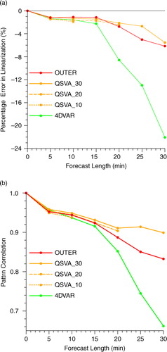
Based on the analyses of the percentage error in linearisation and pattern correlation, it can be seen that the gap between NLG and LG is reduced in the OUTER and QSVA experiments. In the OUTER experiment, as more outer loops are applied, the first guess and nonlinear model trajectory for linearisation are updated. Similarly, in the QSVA experiment, as the length of the assimilation window increases, the first guess and nonlinear model trajectory are updated. Improvement of the first guess and nonlinear model trajectory leads to an improved analysis in the OUTER and QSVA experiments. Furthermore, as the length of the assimilation window increases in the QSVA experiment, the nonlinearity of the original minimisation problem also increases because a high degree of nonlinearity usually results from a lengthy assimilation window, high resolution, and so on.

Table 5 shows the running time for the 4DVAR, OUTER and QSVA experiments on a LINUX cluster with 8 Central Processing Units (CPUs) and 50-GB of memory. The computational cost of the QSVA experiment is greater than that of the 4DVAR experiment, but it is much less than that of the OUTER experiment. This saving in computational time in the QSVA experiment is due to a shorter assimilation window of prior minimisation tasks than in the OUTER experiment. Generally, in operational environments, the computational cost is concentrated near the cut-off time. Through the time-incremental 4D-Var method, some computations can be done before the cut-off time, and hence the computational burden can be distributed efficiently (Järvinen et al., 1996). The computational cost required for the QSVA experiment can be reduced further by using different stopping criterion in the minimisation of the cost function in prior minimisation tasks. In an additional experiment, QSVA_LC, the minimisation of the cost function is finished when the gradient norm is reduced by just one order of magnitude when the length of the assimilation window is 0, 10 or 20 minutes. As the final minimisation task is of our main concern, the prior minimisation tasks need not to be solved precisely, and hence this method to reduce the computational cost can be justified. It is known that the minimisation process acts on the largest scale first (Thépaut and Courtier, 1991; Navon et al., 1992; Tanguay et al., 1995), and hence this method enables the large scale to be resolved by prior minimisation tasks, then the small scales to be sought for only during the final minimisation task. The computational cost of the QSVA_LC experiment is less than for the QSVA experiment by approximately 1 hour. Note that the quality of the analysis and subsequent forecast in the QSVA_LC experiment is very similar to those in the QSVA experiment (not shown).

Table 5 Computing time (hours) and total number of iterations in minimisations of the 4DVAR, OUTER, QSVA and QSVA_LC experiments

	4DVAR	OUTER	QSVA	QSVA_LC
Computing time	7.5	27.25	12.95	12.05
Total number of iterations	21	73	79	55

In the OUTER experiment, the sum of the first, second and third outer loops is shown. Similarly, in the QSVA and QSVA_LC experiments, the sum of assimilation tasks with assimilation window of 0, 10, 20 and 30 minutes is shown.

4.2. Forecast results

Figure 6 shows the 6 hours accumulated rainfall distributions from 0600 UTC to 1200 UTC, 6 August 2006 for the CONTROL, 3DVAR, 4DVAR, OUTER and QSVA experiments. In the CONTROL experiment, there is rainfall over the southwestern part of the Korean Peninsula with maximum rainfall amount of about 62.9 mm (Fig. 6a). However, rainfall distribution is too localised to be regarded as rainfall caused by an organised system, and the 6 hours accumulated rainfall amount is overestimated compared to the observations. When the radar radial velocity data are assimilated using the 3D-Var method, no significant improvement in rainfall distribution can be found compared to the CONTROL experiment (Fig. 6b). In the 4DVAR experiment, rainfall distribution over the southwestern part of the Korean Peninsula is relatively well simulated compared to the CONTROL and 3DVAR experiments. However, the 6 hours accumulated rainfall amount at the southwestern maximum rainfall point (~155.8 mm) is highly overestimated compared to the observations, and the rainfall distribution incorrectly extends to the central part of South Korea. In addition, rainfall over the east coast is not simulated at all in the 4DVAR experiment (Fig. 6c). Rainfall distribution in the OUTER experiment is similar to that in the 4DVAR experiment, but the 6 hours accumulated rainfall amount in the OUTER experiment is even greater than that in the 4DVAR experiment (Fig. 6e). The 6 hours accumulated rainfall distribution in the QSVA experiment is similar to the observations. Both of the localised rainfall maxima in the observations are simulated in the QSVA experiment although the localised rainfall maximum over the east coast is displaced eastward compared to the observations. The 6 hours accumulated rainfall amount at the maximum point over the southwestern part of the Korean Peninsula is approximately 34.2 mm, and that over the east coast is approximately 31.7 mm in the QSVA experiment (Fig. 6d). Both of them are similar to the observations.

Fig. 6 Six hours accumulated rainfall (mm 6 h⁻¹) distribution over South Korea from 0600 UTC to 1200 UTC, 6 August 2006 for the (a) CONTROL, (b) 3DVAR, (c) 4DVAR, (d) QSVA and (e) OUTER experiments. Note that different colour scales are used for the QSVA and OUTER experiments.

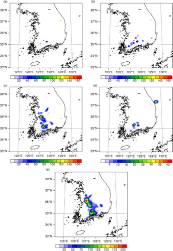
The time series of the hourly rainfall at the southwestern and east coast maxima from 0600 UTC to 1200 UTC, 6 August 2006 for the CONTROL, 3DVAR, 4DVAR, OUTER and QSVA experiments are shown in Fig. 2b and c along with the observations. At the southwestern maximum, the observed rainfall peaked at 1000 UTC with rainfall amount of 30.5 mm, and the rainfall was concentrated around the peak time. In the CONTROL and 3DVAR experiments, the rainfall peak appears at 0800 UTC, and the rainfall amount at the peak time is approximately 47.9 and 59.1 mm, respectively. The peak time is earlier than the observations, and the rainfall amount at the peak time is overestimated compared to the observations. In the 4DVAR experiment, the rainfall peaks at 1000 UTC with rainfall amount of about 78.2 mm. Although the peak time is well simulated, the rainfall amount at the peak time is highly overestimated compared to the observations. This is consistent with the result of the 6 hours accumulated rainfall distribution shown in Fig. 6c. The rainfall peak appears at 0900 UTC (earlier than the observations) with rainfall amount of 47.8 mm (overestimated) in the OUTER experiment. In the QSVA experiment, hourly rainfall peaks at 1000 UTC, which is identical to the observations, although the rainfall amount at the peak time (~21.9 mm) is slightly underestimated compared to the observations. At the east coast maximum, in the observations, rainfall was concentrated around the peak time, 0800 UTC, with rainfall amount of about 34.0 mm. The east coast rainfall maximum is simulated only in the QSVA experiment, as shown in Fig. 6. In the QSVA experiment, rainfall peaks at 0800 UTC like the observations in spite of an underestimation of the rainfall amount at the peak time (~24.6 mm).

To figure out why the rainfall forecast of the QSVA experiment is different from that of the 4DVAR (or OUTER) experiment, analysis increments of the 4DVAR and QSVA experiments are investigated. Figure 7 shows analysis increments of the horizontal wind, divergence and CAPE at 850 hPa for the 4DVAR and QSVA experiments with the corresponding background fields. In the CONTROL experiment (i.e. in background fields), CAPE over the southern part of the Korean Peninsula is greater than 1500 J kg⁻¹, and the water vapour mixing ratio is also large over South Korea. However, in the CONTROL experiment, the rainfall distribution is too localised to be considered as rainfall caused by an organised system (Fig. 6a). In the CONTROL experiment, the horizontal wind over the Yellow Sea and the Korean Peninsula is anti-cyclonic, and divergence is dominant over the southern part of the Korean Peninsula (Fig. 7a). As a result, there is no lift forcing in the CONTROL experiment, which is necessary in simulating rainfall over the southwestern part of the Korean Peninsula. Incremental wind of the 4DVAR experiment is cyclonic and convergent over the Yellow Sea and the southwestern part of the Korean Peninsula. In particular, the analysis increment of convergence is maximised near the southwestern maximum (Fig. 7b). Consequently, through the assimilation of radial velocity data using the 4D-Var method, the horizontal wind over the southwestern part of the Korean Peninsula is modified, and this modification provides continuous forcing for lift, which is necessary for simulating rainfall. However, simulated rainfall over the southwestern part of the Korean Peninsula is highly overestimated, and it extends erroneously to the central part of South Korea in the 4DVAR experiment. This is because the analysis increment of CAPE over the western part of the Korean Peninsula is positive, and excessive convective instability is simulated over that region. Incremental wind in the QSVA experiment over the southwestern part of the Korean Peninsula is cyclonic and convergent as in the 4DVAR experiment. In contrast to the 4DVAR experiment, however, the analysis increment of CAPE over the western part of the Korean Peninsula is negative, and this improves the rainfall forecast over the southwestern part of the Korean Peninsula in the QSVA experiment. It is also noted that in the QSVA experiment, the analysis increment of CAPE over the east coast is positive, and this may enable the simulation of the observed rainfall near the east coast maximum (Fig. 7c).

Fig. 7 (a) Convective available potential energy (CAPE, J kg⁻¹, shading), divergence (10⁻⁵ s⁻¹, negative values are denoted by dashed contours) and winds (m s⁻¹, vector) of 850 hPa at 0600 UTC, 6 August 2006 for the CONTROL experiment. Analysis increments of CAPE (J kg⁻¹, shading), divergence (10⁻⁵ s⁻¹, negative values are denoted by dashed contours) and winds (m s⁻¹, vector) at 850 hPa for the (b) 4DVAR and (c) QSVA experiments.

The analyses of both the OUTER and QSVA experiments are better than the 4DVAR experiment, but the rainfall forecast of only the QSVA experiment is improved. In the OUTER experiment, a 30-minute assimilation window is used in the inner-loop minimisations of all the outer loops. However, in the QSVA experiment, the length of the assimilation window is increased gradually from 0 to 30 minutes, and the nonlinearity of the original minimisation problem is increased accordingly. Therefore, the relatively low-quality first guess is used when the nonlinearity (and chance of multiple minima) of the nonlinear minimisation problem is comparatively low, and vice versa. In other words, by increasing the length of the assimilation window step by step, the orbit minimising the cost function is determined at each step, and that orbit is used as the starting point for the next minimisation in the time-incremental 4D-Var method. This quasi-static adjustment ensures that the computed minimum at every step is the global minimum, and the starting point of the minimisation of the cost function always lies within the attractive basin of the global minimum of the next minimisation (Pires et al., 1996). As a possible measure of closeness to the global minimum, the norm of the gradient vector at the end of cost-function minimisation for the 4DVAR, OUTER and QSVA experiments is computed (Table 6). When the number of applied outer loops is increased, the gradient norm is consistently decreased in the OUTER experiment. In the QSVA experiment, the length of the assimilation window is gradually increased, and hence the gradient norm for the assimilation window of 30 minutes should be compared to the 4DVAR and OUTER experiments. The gradient norm of the QSVA experiment is less than that of the 4DVAR or OUTER experiment, and this implies that the analysis of the QSVA experiment is closer to the global minimum than that of the 4DVAR or OUTER experiment. This is also convincingly shown indirectly by the improved rainfall/meteorological field forecasts of the QSVA experiment.

Table 6 Norm of gradient vector at the end of each cost-function minimization for the 4DVAR, OUTER and QSVA experiments

	4DVAR	OUTER (2)	OUTER (3)	QSVA (0)	QSVA (10)	QSVA (20)	QSVA (30)
Gradient norm	11.468	1.872	1.644	3.200	0.653	1.313	1.611

The number in parenthesis in the OUTER experiment indicates the number of outer loops applied and that in the QSVA experiment indicates the length of the assimilation window (in minute) for each assimilation task.

5. Summary and conclusions

The heavy rainfall case selected in this study is characterised by two localised rainfall maxima over the southwestern part and east coast of the Korean Peninsula. This rainfall was caused by an air-mass thunderstorm related to daytime surface heating. The atmosphere over the southwestern part and the east coast of the Korean Peninsula was convectively unstable with a large CAPE value, and lower-level convergence acted as a lift forcing. When no radar data are assimilated (CONTROL experiment) or when radar data are assimilated using the 3D-Var method (3DVAR experiment), neither of the two localised rainfall maxima is simulated accurately.

By using the 4D-Var method (4DVAR experiment), the simulated rainfall over the southwestern part of the Korean Peninsula is partially improved compared to the CONTROL or 3DVAR experiment. To obtain further improvements to the rainfall forecast, more than one outer loops (OUTER experiment) and the time-incremental 4D-Var method (QSVA experiment) are used. In the QSVA experiment, the length of the assimilation window is increased gradually, and the starting point of the current minimisation task comes from the minimiser of the previous minimisation task.

The ending value of the cost function and RMSE of O−A for the OUTER and QSVA experiments is smaller than those for the 4DVAR experiment. This implies that the analysis of the OUTER and QSVA experiments is closer to the observations than that of the 4DVAR experiment. RMSE of O−B (or O−FG) and RMSD of analysis increment for the OUTER and QSVA experiments are less than those for the 4DVAR experiment, and hence the improved analysis of the OUTER and QSVA experiments is due to a better first guess. Moreover, additional observations, which are rejected in the 4DVAR experiment, get into the assimilation in the OUTER and QSVA experiments although the increase in the number of assimilated observations is not large.

The gap between NLG and LG (or the nonlinearity of the original minimisation problem) is investigated using two measures, namely, the percentage error in linearisation and the pattern correlation. In terms of both the percentage error in linearisation and pattern correlation, the gap between NLG and LG is reduced in the OUTER and QSVA experiments compared to the 4DVAR experiment. This is because the first guess and nonlinear model trajectory are updated progressively in the OUTER and QSVA experiments. It should also be noted that the nonlinearity of the nonlinear minimisation problem is increased with increasing length of the assimilation window in the minimisation tasks of the QSVA experiment.

In the CONTROL and 3DVAR experiments, no organised rainfall is simulated although the atmosphere over the southwestern part of the Korean Peninsula is simulated to be conditionally unstable. Incremental wind in the 4DVAR experiment is cyclonic and convergent over the southwestern part of the Korean Peninsula, which acts as a lift forcing, and this modification to the wind field leads to an improved rainfall forecast in the 4DVAR experiment compared to the CONTROL or 3DVAR experiment. However, the 6 hours accumulated rainfall amount over the southwestern part of the Korean Peninsula is overestimated, and the rainfall distribution extends wrongly to the central part of South Korea in the 4DVAR experiment. The simulated rainfall in the OUTER experiment is similar to that in the 4DVAR experiment except for more excessive rainfall amount. In the QSVA experiment, the analysis increment of CAPE is negative (positive) over the western part (east coast) of the Korean Peninsula, which results in a better rainfall forecast than in the 4DVAR and OUTER experiments. Besides rainfall forecast, forecasts of other meteorological fields such as wind, temperature and water vapour mixing ratio are improved in the QSVA experiment (not shown). Analyses of both the OUTER and QSVA experiments are improved compared to that of the 4DVAR experiment, but the rainfall forecast of only the QSVA experiment is improved. In the QSVA experiment, the nonlinearity of the original minimisation problem is increased gradually with increasing length of the assimilation window. This quasi-static adjustment guarantees that the computed minimum at the current minimisation is the global minimum (or close to the global minimum) and the starting point for the next minimisation lies within the basin of the global minimum.

Consequently, the quality of the analysis is improved in the OUTER and QSVA experiments compared to the 4DVAR experiment owing to the nonlinear model trajectory and first guess being updated. However, the rainfall forecast is improved only in the QSVA experiment due to modifications in the analysis. The quasi-static adjustment of the time-incremental 4D-Var method leads to an improved analysis in spite of the high degree of nonlinearity of this heavy rainfall case. In addition, the computational cost of the time-incremental 4D-Var method is much smaller than that of using multiple outer loops, and it can be further reduced through the use of a loose stopping criterion for the inner-loop minimisation. The conclusions of this study cannot be generalised because the time-incremental 4D-Var method has been applied to only one particular case (i.e. this is a case study). However, it is expected that the time-incremental 4D-Var method will be more effective when the length of the assimilation window is increased and the nonlinearity of the minimisation problem is increased accordingly. The time-incremental 4D-Var method will be applied to other heavy rainfall cases over the Korean Peninsula and the results will be reported as another article.

Acknowledgments

This work was funded by the Korea Meteorological Administration Research and Development Program under Grant CATER 2012-6080. The authors thank the anonymous reviewers for their valuable comments.

Notes

¹The structure of the background error covariance derived from the NMC method may not be appropriate for assimilation of radar data. Lee et al. (2010) pointed out that length scale for radial velocity or reflectivity should be tuned using, for example, Hollingsworth and Lönnberg (1986)'s method to assimilate high-resolution Doppler radar data more efficiently. However, tuning of length scale is beyond the scope of this study, and hence this aspect will not be discussed any more.

²When comparing the ending value of the cost function in the current outer loop with the starting value of the cost function in the following outer loop, there is a jump-up. This is attributed to two factors: the first is the nonlinearity of the forecast model and/or observation operator, and the second is additional observations getting into the assimilation, which are rejected in the previous outer loop.

References

- Courtier P , Thépaut J.-N , Hollingsworth A . A strategy for operational implementation of 4D-Var, using an incremental approach. Q. J. Roy. Meteorol. Soc. 1994; 120: 1367–1387.
- Daley R , Barker E . The NAVDAS Source Book. 2001; NRL/PJ/7530-01-441. Naval Research Laboratory, Monterey, California. 163.
- Dudhia J . Numerical study of convection observed during the winter monsoon experiment using a mesoscale two-dimensional model. J. Atmos. Sci. 1989; 46: 3077–3107.
- Evensen G . Sequential data assimilation with a nonlinear quasi-geostrophic model using Monte Carlo methods to forecast error statistics. J. Geophys. Res. 1994; 99C5: 10143–10162.
- Gandin L. S . Objective analysis of meteorological fields. 1963; Translated from Russian 1965, Israel program for scientific translations, Jerusalem. 242.
- Gauthier P , Tanguay M , Laroche S , Pellerin S . Extension of 3DVAR to 4DVAR: implementation of 4DVAR at the Meteorological Service of Canada. Mon. Weather. Rev. 2007; 135: 2339–2364.
- Gauthier P , Thépaut J.-N . Impact of the digital filter as a weak constraint in the preoperational 4DVAR assimilation system of Météo France. Mon. Weather Rev. 2001; 129: 2089–2102.
- Haben S. A , Lawless A. S , Nichols N. K . Conditioning of incremental variational data assimilation, with application to the Met Office system. Tellus A. 2011; 63: 782–792.
- Haltiner G. J , Williams R. T . Numerical Prediction and Dynamic Meteorology. 1980; Wiley, New York. 477.
- Hollingsworth A , Lönnberg P . The statistical structure of short-range forecast errors as determined from radiosonde data. Part I: the wind field. Tellus A. 1986; 38: 111–136.
- Honda Y , Nishijima M , Koizumi K , Ohta Y , Tamiya K . A pre-operational variational data assimilation system for a non-hydrostatic model at the Japan Meteorological Agency: formulation and preliminary results. Q. J. Roy. Meteorol. Soc. 2005; 131: 3465–3475.
- Hong S.-Y , Lim J.-O . The WRF single-moment 6-class microphysics scheme (WSM6). J. Korean Meteorol. Soc. 2006; 42: 129–151.
- Hong S.-Y , Noh Y , Dudhia J . A new vertical diffusion package with an explicit treatment of entrainment processes. Mon. Weather Rev. 2006; 134: 2318–2341.
- Huang X.-Y , Yang X , Gustafsson N , Mogensen K , Lindskog M . Four-dimensional variational data assimilation for a limited area model. HIRLAM Tech Rep. 2002; 57: 41. [Available from SMHI, S-601 76 Norrkoping, Sweden.].
- Huang X.-Y , Xiao Q , Barker D. M , Zhang X , Michalakes J . Four-dimensional variational data assimilation for WRF: formulation and preliminary results. Mon. Weather Rev. 2009; 137: 299–314.
- Järvinen H , Thépaut J.-N , Courtier P . Quasi-continuous variational data assimilation. Q. J. Roy. Meteorol. Soc. 1996; 122: 515–534.
- Kain J. S . The Kain–Fritsch convective parameterization: an update. J. Appl. Meteorol. 2004; 43: 170–181.
- Le Dimet F , Talagrand O . Variational algorithms for analysis and assimilation of meteorological observations: theoretical aspects. Tellus A. 1986; 38: 97–110.
- Lee J.-H , Lee H.-H , Choi Y , Kim H.-W , Lee D.-K . Radar data assimilation for the simulation of mesoscale convective systems. Adv. Atmos. Sci. 2010; 27: 1025–1042.
- Lewis J , Derber J . The use of adjoint equations to solve a variational adjustment problem with advective constraints. Tellus A. 1985; 37: 309–327.
- Lorenz E. N . Deterministic nonperiodic flow. J. Atmos. Sci. 1963; 20: 130–141.
- Miller L. J , Mohr C. G , Weinheimer A. J . The simple rectification to Cartesian space of folded radial velocities from Doppler radar sampling. J. Atmos. Ocean. Tech. 1986; 3: 162–174.
- Mlawer E. J , Taubman S. J , Brown P. D , Iacono M. J , Clough S. A . Radiative transfer for inhomogeneous atmospheres: RRTM, a validated correlated-k model for the longwave. J. Geophys. Res. 1997; 102: 16663–16682.
- Mohr C. G , Vaughan R. L . An economical procedure for Cartesian interpolation and display of reflectivity data in three dimensional space. J. Appl. Meteorol. 1979; 18: 661–670.
- Mohr C. G , Vaughan R. L , Frank H. W . The merger of mesoscale datasets into a common Cartesian format for efficient and systematic analyses. J. Atmos. Ocean. Tech. 1986; 3: 144–161.
- Navon I. M , Zou X , Derber J , Sela J . Variational data assimilation with an adiabatic version of the NMC spectral model. Mon. Weather Rev. 1992; 120: 1433–1446.
- Park S.-G , Lee D.-K . Retrieval of high-resolution wind fields over the Southern Korean Peninsula using the Doppler weather radar network. Weather Forecast. 2009; 24: 87–103.
- Parrish D. F , Derber J . The National Meteorological Center's spectral statistical-interpolation analysis system. Mon. Weather Rev. 1992; 120: 1747–1763.
- Pires C , Vautard R , Talagrand O . On extending the limits of variational assimilation in nonlinear chaotic systems. Tellus A. 1996; 48: 96–121.
- Rabier F , Järvinen H , Klinker E , Mahfouf J.-F , Simmons A . The ECMWF operational implementation of four-dimensional variational assimilation. Experimental results with simplified physics. Q. J. Roy. Meteorol. Soc. 2000; 126: 1143–1170.
- Rawlins F , Ballard S. P , Bovis K. J , Clayton A. M , Li D . The Met Office global 4-Dimensional data assimilation system. Q. J. Roy. Meteorol. Soc. 2007; 133: 347–362.
- Rizvi S. R. H , Guo Y.-R , Shao H , Demirtas M , Huang X.-Y . Impact of outer loop for WRF data assimilation system (WRFDA). Proceedings of the 9th WRF Users’ Workshop. 2008; CO: National Center for Atmospheric Research (NCAR), Boulder.
- Talagrand O . Assimilation of observations, an introduction. J. Meteorol. Soc. Japan. 1997; 75: 191–209.
- Tanguay M , Bartello P , Gauthier P . Four-dimensional data assimilation with a wide range of scales. Tellus A. 1995; 47: 974–997.
- Thépaut J.-N , Courtier P . Four-dimensional variational data assimilation using the adjoint of a multilevel primitive-equation model. Q. J. Roy. Meteorol. Soc. 1991; 117: 1225–1254.
- Trémolet Y . Diagnostics of linear and incremental approximations in 4D-Var. Q. J. Roy. Meteorol. Soc. 2004; 130: 2233–2251.
- Skamarock W. C , Klemp J. B , Dudhia J , Gill D. O , Barker D. M , co-authors . A description of the Advanced Research WRF version 3. 2008. NCAR Tech. Note TN-475+STR, 113.
- Sun J , Chen M , Wang Y . A frequent-updating analysis system based on radar, surface, and mesoscale model data for the Beijing 2008 forecast demonstration project. Weather Forecast. 2010; 25: 1715–1735.
- Sun J , Crook A . Dynamical and microphysical retrieval from Doppler radar observations using a cloud model and its adjoint. Part I: model development and simulated data experiments. J. Atmos. Sci. 1997; 54: 1642–1661.
- Sun J , Crook A . Dynamical and microphysical retrieval from Doppler radar observations using a cloud model and its adjoint. Part II: retrieval experiments of an observed Florida convective storm. J. Atmos. Sci. 1998; 55: 835–852.
- Wang H , Sun J , Zhang X , Huang X.-Y , Auligné T . Radar data assimilation with WRF 4D-Var: part I. System development and preliminary testing. Mon. Weather Rev. 2013; 141: 2224–2244.
- Xiao Q , Kuo Y.-H , Ma Z , Huang W , Huang X.-Y . Application of an adiabatic WRF adjoint to the investigation of the May 2004 McMurdo, Antarctica, severe wind event. Mon. Weather Rev. 2008a; 136: 3696–3713.
- Xiao Q , Kuo Y.-H , Sun J , Lee W.-C , Barker D. M . An approach of radar reflectivity data assimilation and its assessment with the inland QPF of typhoon Rusa (2002) at landfall. J. Appl. Meteorol. Clim. 2007; 46: 14–22.
- Xiao Q , Kuo Y.-H , Sun J , Lee W.-C , Lim Y.-R . Assimilation of Doppler radar observations with a regional 3DVAR system: impact of Doppler velocities on forecasts of a heavy rainfall case. J. Appl. Meteorol. 2005; 44: 768–788.
- Xiao Q , Sun J . Multiple-radar data assimilation and short-range quantitative precipitation forecasting of a squall line observed during IHOP_2002. Mon. Weather Rev. 2007; 135: 3381–3404.
- Xiao Q , Lim E , Won D.-J , Sun J , Lee W.-C . Doppler radar data assimilation in KMA's operational forecasting. Bull. Am. Meteorol. Soc. 2008b; 89: 39–43.
- Xu L , Rosmond T , Daley R . Development of NAVDAS-AR: formulation and initial tests for the linear problem. Tellus A. 2005; 57: 546–559.
- Zhang X , Huang X.-Y , Pan N . Development of the upgraded tangent linear and adjoint of the Weather Research and Forecasting (WRF) model. J. Atmos. Ocean. Tech. 2013; 30: 1180–1188.