Double Fourier series dynamical core with hybrid sigma-pressure vertical coordinate

Abstract

The hybrid sigma-pressure vertical coordinate is implemented into the double Fourier series (DFS) dynamical core of the Global/Regional Integrated Model system (GRIMs). Using traditional verification metrics, the model is quantitatively compared to a model that uses the terrain-following sigma coordinate. The distribution and skill scores for precipitation simulated with the hybrid coordinate are not significantly different from those found using the sigma coordinate. The hybrid coordinate has a positive effect on medium-range forecast skill in terms of geopotential height and temperature, especially in the tropics and upper layers of the atmosphere. Furthermore, the root-mean-squared error for relative humidity is significantly reduced near 100 hPa in the Northern (Southern) Hemisphere for a boreal summer (winter). The effect of the hybrid coordinate is found to be almost the same in the GRIMs-spherical harmonics (SPH) dynamical core. For the GRIMs-DFS dynamical core, the hybrid coordinate is insensitive to the abrupt transition of diffusivity at approximately 100 hPa, where numerical diffusion errors occur with the sigma coordinate. This suggests that the hybrid coordinate is necessary for the unique horizontal diffusion method of the GRIMs-DFS dynamical core.

• hybrid sigma-pressure vertical coordinate
• global atmospheric model
• double Fourier series
• spectral method
• GRIMs

1. Introduction

The spectral transform method has been widely used as the basis for the dynamical core of numerical weather prediction (NWP) and climate models as it has significant computational advantages over finite-difference methods such as its high numerical accuracy, uniform resolvability, and ease of Laplacian operation (Cheong, 2006; Williamson, 2007). However, spectral methods suffer from low scalability because they must use non-local calculations for wave to grid (or vice versa) transformation and, more importantly, from high computational cost, as the Legendre transform in traditional spherical harmonics (SPH) requires O[N³] operations, with N being the truncated wave number (Williamson et al., 1992; Cheong, 2000b, 2000a; Williamson, 2007). Although many efforts have been made to alleviate computational inefficiencies in the field of global spectral modelling (e.g. Taylor et al., 1997; Juang, 2004; Tygert, 2010), they have not resolved the defects inherent in the SPH dynamical core that result in elevated computational cost at high resolution.

The use of the double Fourier series (DFS) as an orthogonal basis function is an alternative method in spectral representation because a fast algorithm is available when transforming from the wave to the grid domain and vice versa, and most of the advantages of the traditional spectral method are preserved more effectively than with the grid-point method (Cheong, 2000b, 2000a; Layton and Spotz, 2003; Cheong, 2006). The DFS approach requires an equally spaced latitude grid instead of a Gaussian distribution, utilises fast-Fourier-transforms (FFTs) in the latitude direction, rather than the more computationally expensive Legendre transforms, and offers reduced computational cost characterised by O[N²log₂N]. Cheong (2000b) proposed a new DFS method for solving simple elliptic equations and vorticity and advection equations on a sphere. This was extended to the shallow-water model by Cheong (2000a) and was evaluated satisfactorily using the standardised test for dynamical cores. Along with the development of a high-order harmonic spectral filter by DFS (Cheong et al., 2002; Cheong et al., 2004), Cheong (2006) – (hereafter C2006) further extended the DFS spectral method to a three-dimensional atmospheric model with hydrostatic approximation on sigma vertical coordinate (SIG). C2006 reported that the new method retains most of the advantages of the traditional spectral method and provides an efficient and simple high-order filtering method that is essential for stable time stepping. Additionally, the DFS approach was found to have greater computational efficiency than the SPH model in cases of higher model resolution.

Park et al. (2013) – (hereafter P2013) implemented the DFS method reported by C2006 into a global spectral model based on the SPH dynamical core with full physics packages. In this process, the DFS algorithm was parallelised using a message-passing interface (MPI) library routine. Specific humidity was added as a prognostic variable for water conservation, which was absent in C2006. They demonstrated that, compared to the traditional SPH model, the DFS model with full physics does not exhibit discernible deficiencies in terms of the accuracy of the simulated climatology and the forecast of a heavy rainfall event. Most importantly, the parallelised DFS algorithm also guaranteed computational efficiency in the cluster computer with increases in model resolution, which is consistent with the theoretical performance computed from a dry primitive equation model framework by C2006.

For a vertical finite-difference scheme, C2006 and P2013 adopted the terrain-following SIG system, first introduced by Phillips (1957), which has been widely used in both global and regional atmospheric models because it follows natural near-ground terrain and derives the governing equations more simply than other vertical coordinate systems. However, it has been shown that, in the upper levels of the atmosphere, horizontal pressure gradient errors can be induced by forcing the coordinate surfaces to transform to pressure surfaces in levels as low as 400 hPa over steep orography (Janjic, 2004). Moreover, small-scale structures in the coordinate surfaces render advection computation inaccurate (Schär et al., 2002; Zängl, 2003).

To correct these numerical defects, a hybrid vertical coordinate system has been designed with a combination of sigma levels near the ground and isobaric levels at higher elevation (Arakawa and Lamb, 1977; Simmons and Burridge, 1981), which has become standard in NWP (e.g. Allen et al., 2006; Sela, 2009; White, 2011) and climate (e.g. Roeckner et al., 2003; Collins et al., 2004) models. Eckermann (2009) – (hereafter E2009) compared the wide variety of hybrid coordinate systems currently used in operational global models and proposed a new hybrid coordinate system focusing on the properties of the vertical derivative of the terrain-following coefficient. In addition, E2009 reported that the hybrid coordinate generally offers improved forecast skill relative to that offered by the traditional sigma coordinate. Despite its widespread use, it has been reported that the hybrid coordinate system causes a decrease in the stability of the semi-implicit scheme (Simmons and Burridge, 1981), although this trade-off has only a weak effect on forecast skill (cf. E2009). For this reason, before E2009, there was no in-depth evaluation of hybrid coordinate systems in terms of forecast skill presented in the literature.

The purpose of this study is to implement a hybrid sigma-pressure vertical coordinate into the DFS dynamical core and to assess its performance at different horizontal resolutions on various time scales, with a particular focus on traditional medium-range forecast skill. The effect of the hybrid coordinate is quantitatively examined and is contrasted with the terrain-following sigma coordinate. The next section briefly describes the spectral model employed herein and presents the governing equations and properties related to the hybrid coordinate. Section 3 describes the experimental setup. Results are discussed in Section 4. Concluding remarks are given in the final section.

2. Implementation

2.1. A brief model description

The Global/Regional Integrated Model system (GRIMs) (Hong et al., 2013) is a multi-scale atmospheric modelling system with unified physics, which has been created for use in NWP, seasonal simulations, and climate research on global and regional scales. The initial version of the global and regional model is rooted in the National Centres for Environmental Prediction (NCEP) seasonal forecast model (Kanamitsu et al., 2002b) and regional spectral model (Juang et al., 1997), but subsequent versions have benefited from developments to the model's physics and dynamics, along with a reconfiguration of the code structure. The GRIMs has great multi-platform flexibility in either thread mode or MPI mode. In addition to the SPH dynamical core for the global model, the DFS method from C2006 is available as another dynamical core (P2013). In addition, a single-column model is devised for effective evaluation of the physics algorithms, and the Geophysical Fluid Dynamics Laboratory (GFDL) Modular Ocean Model version 3 (MOM3) (Pacanowski and Griffies, 1998) is coupled with the GRIMs for climate prediction and mechanism studies.

The system has multiple options in each physics parameterisation. The physics packages used in this study (GRIMs version 3.0) include short- and long-wave radiative parameterisation, land surface model, diagnostic microphysics, convective parameterisation, gravity wave drag by orography and convection, and a vertical diffusion package. In addition, the diurnal variation of sea surface temperature (SST) is taken into account by incorporating an ocean mixed layer model and a surface energy budget for skin temperature. More details may be found in Hong et al. (2013).

2.2. Governing equations

Derivation of the hybrid sigma-pressure vertical coordinate is based on publications related to the NCEP Global Forecast System (GFS) (Sela, 2009) and European Centres for Medium-range Weather Forecast (ECMWF) (White, 2011) spectral models using the SPH dynamical core. For the GRIMs-DFS dynamical core, however, the derivation is not as straightforward as for the SPH dynamical core due to the different prognostic variables in the primitive equation set. For example, while the GRIMs-SPH dynamical core uses wind components and virtual temperature in the momentum and thermodynamic equations, respectively, the GRIMs-DFS dynamical core uses vorticity/divergence and perturbation of virtual temperature in the corresponding equations. Based on C2006, primitive equations with the hybrid coordinate are newly devised for the DFS dynamical core in the flux-form and are defined as:1a 1b 1c 1d 1e

and1f

where2a 2b

where ζ, D, , q, and Φ represent the vorticity, divergence, perturbation of virtual temperature, specific humidity, and geopotential, respectively; and θ are the longitude and latitude, respectively; u and v are the velocity components in longitude and latitude, respectively; , p and p _s are the pressure and surface pressure, respectively; a, Ω, R _d , and are the radius of the Earth, angular velocity of the Earth, gas constant for dry air, and Coriolis parameter, respectively; , with C _p =1004.6 as the specific heat capacity of dry air at constant pressure; , with R _v as the gas constant for water vapour; , with C _pv as the specific heat capacity of water vapour at constant pressure; η is the generalised vertical coordinate at the interface layer; and and are the pressure- and hybrid-coordinate vertical velocities at the interface layer, respectively. The term K in eqs. (1a)–(1d) denotes the horizontal scale-dependent viscosity or diffusivity. Detailed procedures of semi-implicit time stepping and numerical discretisation are well described in C2006 and Sela (2009), so they are not repeated in this paper.

2.3. Configuration of hybrid co-ordinate

The generalised hybrid coordinate can be defined by the vertical profiles of the two coefficients, A and B, which control, respectively, the isobaric and terrain-following properties (Simmons and Strüfing, 1983) as shown below:3 where is the corresponding vertical profile of η values for p _s =p ₀, where p ₀ is the nominal sea level pressure, typically ~1000 hPa; and P _top is the pressure at the highest interface layer, typically 0 hPa. In the discretised form, is given by:4 where k−1/2 indicates the interface layer (or half level) for k=0,1,···,K, with K being the total number of model layers. At each interface layer, the pressure is defined as . If the coefficients A and B are set to pressure and zero, respectively, then eq. (3) becomes a generalisation of the original terrain-following sigma (σ) coordinate. The characteristics of the hybrid coordinate depend upon the coefficient definitions, and the stability of the semi-implicit time scheme is sensitive to the reference pressure and temperature selected for and used in linearisation for time integration. Nevertheless, there is no specific guidance on choosing the governing coefficients that will provide the appropriate hybrid coordinate (see E2009).

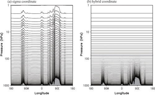
In this study, the properties related to hybrid coordinate are determined in accordance with the conventions of the NCEP GFS model. Reference pressure and temperature are defined as 800 hPa and 300 K, respectively. Figure 1 compares the coordinate surfaces around a 34.5°N latitude circle for the sigma and hybrid vertical coordinates at T254L64 resolution; T254L64 designates that the truncated total (zonal) wave number for the SPH (DFS) is 254 with the vertical layer of 64. The surfaces in the sigma coordinate system follow the topographic elevations and are steeply sloped in regions where orography exists (Fig. 1a). Unlike isobaric or isentropic coordinates, this eliminates the problem of vertical coordinate systems intersecting the ground. While the sigma levels slope remarkably over steep orography, even in the stratosphere, the hybrid coordinate system smoothly changes coordinate surfaces from terrain-following levels near the ground to isobaric surfaces in the upper troposphere or lower stratosphere (Fig. 1b). Above 68 hPa, coordinate surfaces lie in pure pressure coordinates, and the pressure gradient force is easily calculated as the geopotential gradient without any consideration for the coordinate system.

Fig. 1 Vertical profile of coordinate surface versus pressure at 34.5°N for the (a) sigma and (b) hybrid vertical coordinates at T254L64 resolution. Topographic elevations are shaded light gray. The gray contour in (b) shows the lowest-altitude isobaric level (~68 hPa).

3. Experimental setup

In P2013, the DFS dynamical core with full physics was successfully evaluated against a conventional SPH dynamical core in terms of a short-range and seasonal forecast framework. The control DFS experiment with SIG is performed on test-beds identical to those employed by P2013, with the exception of some minor revision to the physics package, and the DFS simulation with the hybrid sigma-pressure vertical coordinate (HYB) is quantitatively compared to the SIG run. The SPH simulation is also conducted on sigma and hybrid vertical coordinates (SIGsph and HYBsph) in order to more closely inspect the coordinate dependency of the dynamical core (Table 1).

Table 1. Summary of experiments

Dynamical core	Vertical coordinate	Physics package
SIG	DFS	Sigma
HYB	DFS	Hybrid	GRIMs
SIGsph	SPH	Sigma	version 3.0
HYBsph	SPH	hybrid

A description of the three test cases is summarised in Table 2. For short-range and seasonal forecasting, the horizontal resolutions are T510L64 (~25 km) and T126L28 (~100 km), respectively. The initial conditions are taken from the NCEP-Department of Energy (DOE) Atmospheric Model Intercomparison Project (AMIP) II reanalysis data (RA2) (Kanamitsu et al., 2002a), and the observed SST is updated daily from the optimal interpolation SST weekly data set (Reynolds and Smith, 1994). To avoid introducing uncertainties from the initial data on a seasonal forecast time scale, five-member ensemble runs for each experiment are performed with an approximate 4-week lead-time for a boreal summer. For deterministic verification on a medium-range time scale, 10-d forecasts are carried out at T254L64 (~50 km) resolution using the NCEP GFS final analysis as the initial fields for a single month of each boreal summer and winter. The verification regions are categorised into the Northern Hemisphere (20°N–90°N), tropics (20°S–20°N), and Southern Hemisphere (20°S–90°S).

Table 2. A summary of test cases

Short-range forecast	Medium-range forecast	Seasonal simulation
Start time	00 UTC for 14 July 2001	Every 00, 12 UTC for August 2010 and for January 2011	00 UTC for 1–5 May 1996 (5-memberensemble)
Integration/Evaluation period	24 hours/last 18 hours	10 d/last 9 d	4 months/last 3 months
Resolution	T510L64 (~25 km)	T254L64(~50 km)	T126L64 (~100 km)
Initial data	NCEP RA2	NCEP GFS-final	NCEP RA2
Evaluation	Heavy rainfall	Deterministic forecast skill	Seasonal climatology

Skill scores for bias, root-mean-squared error (RMSE), pattern correlation coefficient (PCC), and anomaly correlation coefficient (ACC) are calculated at each grid point using conventional verification metrics recommended by the World Meteorological Organisation (WMO, 2012), against analysis data such as the Climate Prediction Centre (CPC) Merged Analysis of Precipitation (CMAP) (Xie and Arkin, 1997) data, the Tropical Rainfall Measuring Mission (TRMM) Multisatellite Precipitation Analysis (TMPA) (Huffman et al., 2007; Koo et al., 2009) data, or the ECMWF Reanalysis (ERA) Interim (Dee et al., 2011) data. Based on the July 2011 updated standard verification procedures (http://www.ecmwf.int/products/forecasts/wmolcdnv/revised_procedures_2011.pdf), resolution of the grid used for verification is changed from 2.5×2.5 to 1.5×1.5, and daily climatology of the ERA-Interim analysis from 1989 to 2008 is used to compute the ACC score. The scores are defined as:5a 5b 5c

and5d where the summations are performed over all grid points for the analysis zone of interest; N is the total number of grid points included in the region; x _f , x _a , and x _c are the forecast, corresponding verifying (analysed), and daily climatological values, respectively; ϕ _i is the latitude of grid point i, and the bars denote spatial averaging within a region. The normalised difference in RMSE (ACC) is obtained by dividing the RMSE (ACC) difference between two experiments by their sum. Then, the normalised difference ranges from −1 to 1.

4. Results and discussion

Previous studies have reported that the semi-implicit time step becomes less stable when a hybrid coordinate is used, and that its stability is sensitive to the reference pressure selected for linearising semi-implicit time integration (Simmons and Burridge, 1981). E2009 showed that a reference pressure of 800 hPa yields the highest overall stability in a semi-implicit time scheme for all the hybrid coordinates tested. In this study, at a fixed reference pressure, all the experiments are stably integrated for the 120, 240, and 600 second time steps for T510L64, T254L64, and T126L28 resolutions, respectively. Additional stability testing is omitted and left for future study.

4.1. Heavy rainfall and seasonal precipitation

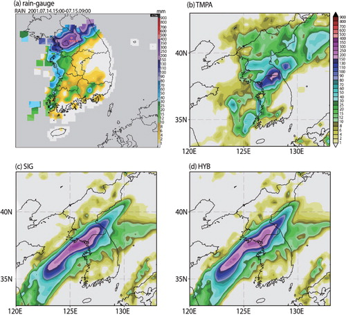
In this section, simulations are evaluated in terms of precipitation, one of the most difficult variables to simulate, on short-range and seasonal forecast time scales. Figure 2 shows the amount of 18-hour accumulated rainfall obtained from rain-gauge and TMPA observations on 15 July 2001 and compares the corresponding precipitation (within a 1-d forecast) simulated from the SIG and HYB runs at an approximately 25 km horizontal resolution. A significant amount of precipitation was recorded, with a local maximum of approximately 371.5 mm near Seoul (Fig. 2a). In Fig. 2b, the TMPA observation exhibits an oceanic precipitation pattern that is not captured by the overland rain-gauge. Compared to the observations, the SIG run follows the observed distribution over South Korea, especially with respect to the local maximum on the west coast of the peninsula (Fig. 2c). Close inspection, however, reveals that the SIG run yields a reduced local maximum (329.2 mm) and a united precipitation core that is separated in the TMPA observations. In terms of precipitation distribution, there is little discrepancy between the SIG and HYB runs (cf. Fig. 2c and 2d); however, in the HYB run, the precipitation core is better separated. This is also in line with the simulation results of the SPH dynamical core (not shown). However, the local maximum in the domain is found to be more reduced in the HYB run (297.8 mm). Statistical validation scores of bias, RMSE, and PCC for 18-hour accumulated precipitation over the East Asian region (100°–150°E, 20°–50°N) reveal that there is little discrepancy in the simulated precipitation in terms of the RMSE and the PCC, but the overland skill scores are slightly lower in the HYB run (not shown).

Fig. 2 Amount of 18-hour accumulated rainfall (mm) obtained from the (a) rain-gauge over South Korea and (b) TMPA data over the Korean peninsula and simulated from the (c) SIG and (d) HYB runs at T510L64 resolution.

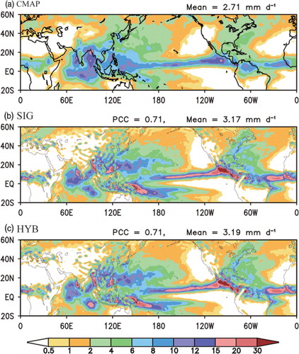
Seasonal simulations for the boreal summer in June–July–August (JJA) of 1996, in which the SST over the equatorial Pacific is a normal condition, are also performed with a five-member ensemble initialised at 0000 Coordinated Universal Time (UTC) for the period of 1–5 May with a 1-d interval at a resolution of approximately 100 km. Figure 3 compares the JJA precipitation from the CMAP data and from the SIG and HYB runs. It is clear that the SIG run satisfactorily reproduces the tropical rainfall comparable to the observations of the main rain-belt along the Intertropical Convergence Zone (ITCZ) over the Pacific and Atlantic, albeit with exaggerated precipitation in terms of global mean (2.71 vs. 3.17 mm d⁻¹) and the double ITCZ (Fig. 3b), which is a deficiency common among many general circulation models (Covey et al., 2003; Dai, 2006). Compared to the SIG run, the HYB run produces more precipitation in the tropics (Fig. 3c). However, the overestimation is not significant in terms of global mean (3.17 vs. 3.19 mm d⁻¹), and the overall feature does not differ much between the two runs. Similar levels of consistency in simulating seasonal precipitation can be ascertained around the globe by the same PCC of 0.71.

Fig. 3 June–July–August (JJA) precipitation (mm d^-1) for 1996, obtained from the (a) CMAP precipitation data and simulated from the (b) SIG and (c) HYB runs at T126L28 resolution.

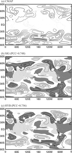
Figure 4 shows the 500 hPa geopotential height standing eddy for the summer of 1996. A standing eddy, also known as a stationary eddy, is defined as the time-averaged departure value from a zonal mean at a latitude and is used to validate a model's general performance (Seol and Hong, 2009). The SIG run generally well reproduces the RA2 eddy in the mid-latitudes of the Northern Hemisphere, including positive-negative anomalies in North America (cf. Fig. 4a and 4b). Separate positive anomalies in the Asian and European continents are better simulated by the HYB run (Fig. 4c). In the Southern Hemisphere, positive anomaly patterns are reproduced well, although the intensification of a negative anomaly is somewhat weakened in the HYB run. The corresponding PCCs against the RA2 are 0.748 and 0.756 for the SIG and HYB runs, respectively. Another evaluation of the upper-level structures (e.g. pressure-latitude cross-sections of the zonally averaged zonal wind, temperature, and humidity) shows a comparable climatology without a discernible difference between the SIG and HYB runs (not shown).

Fig. 4 Same as Fig. 3 but for 500 hPa geopotential height eddy (contour; m). Shading indicates the 95% confidence level.

4.2. Medium-range forecast

Deterministic verification on a medium-range time scale is performed to examine the improvement of large-scale features against the ERA-Interim analysis data. Forecasts are initialised at 0000 and 1200 UTC for each day in the periods of 1–31 August 2010 and 1–31 January 2011. The verification scores against the NCEP GFS data showed only minor differences save for the relative humidity score, which showed relatively high skill scores (not shown). The geopotential height ACC found using the ERA-Interim daily climatology data in accordance with the July 2011 updated verification procedure is significantly lower in the tropics than that found using the NCEP GFS monthly climatology data. For other regions, however, the skill scores achieved by the two methods do not differ significantly.

Figure 5 shows the normalised differences in the RMSE and the ACC of geopotential heights at 850, 500, and 250 hPa between the HYB and SIG runs for initialisations at 0000 UTC in August 2010. A negative (positive) normalised difference in RMSE (ACC) indicates better forecast skill for the HYB runs compared to the SIG runs. At 850 hPa, the RMSE is not significantly different between the SIG and HYB runs for any of the forecast times (Fig. 5a). In the higher model layers, the HYB run demonstrates a clear forecast improvement in RMSE scores (Fig. 5b and 5c). In particular, the RMSE is remarkably reduced in the upper layer of the tropics. The skill improvement, albeit exiguous, is still confirmable in the Northern and Southern Hemispheres up to day 6, when the ACC is approximately 0.7. In terms of ACC (Fig. 5d–Fig. 5f), the improvement in the tropics is discernible, especially at 250 hPa. In the Northern and Southern Hemispheres, the ACCs of the SIG and HYB runs are virtually the same at all layers up to forecast day 6, but thereafter the ACCs are slightly improved by the HYB run. The forecasts for a boreal winter (i.e. January 2011) also yield the same results irrespective of the 0000 and 1200 UTC starting time (not shown).

Fig. 5 Normalised difference in (left) RMSE and (right) ACC of (a),(d) 850, (b),(e) 500, and (c),(f) 250 hPa geopotential heights between the HYB and SIG runs (i.e. HYB minus SIG). The 31-ensemble members initialised at 0000 UTC are averaged at each forecast time during August 2010 and the verification is against the ERA Interim analysis in the northern hemisphere (dashed), tropics (solid), and southern hemisphere (dotted).

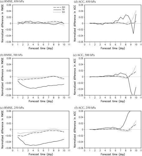
The clear conclusion that can be drawn from Table 3 is that forecast skill for the 5-d forecast is distinctly improved in terms of the 500 hPa geopotential height and temperature, as determined by conventional verification metrics. In terms of geopotential height, the HYB run generally provides higher forecast skill than the SIG run, with the exception of the tropics ACC at 1200 UTC. While the impact of the hybrid coordinate on forecast skill is neutral or weakly positive for geopotential height, the forecast skill for temperature is very high in the HYB run irrespective of season and region. In particular, there is a striking improvement in the tropics, that is, a decrease in RMSE and an increase in ACC of approximately 4–5% and 1–2%, respectively.

Table 3. Skill scores of the RMSE/anomaly correlation coefficient (ACC) for 500 hPa geopotential height (GPH) and temperature (TMP) at 5 d forecast from the SIG and HYB runs, against the ERA Interim analysis data in the northern hemisphere, tropics, and southern hemisphere. Better scores are highlighted in bold.

August 2010		January 2011
Variable	Experiment	00UTC	12UTC	00UTC	12UTC
Northern Hemisphere
SIG	45.5/0.815	44.9/0.818	61.8/0.850	64.1/0.840
HYB	44.9/0.817	44.4/0.821	61.1/0.853	63.6/0.842
Tropics
GPH	SIG	23.7/0.515	24.2/0.528	25.0/0.628	25.1/0.648
HYB	22.2/0.519	22.6/0.526	23.4/0.630	23.9/0.643
Southern Hemisphere
SIG	76.3/0.785	75.4/0.796	56.8/0.821	56.9/0.817
HYB	76.0/0.786	75.0/0.798	56.7/0.821	56.9/0.817
Northern Hemisphere
SIG	2.47/0.925	2.45/0.928	2.98/0.956	3.04/0.954
HYB	2.43/0.925	2.41/0.928	2.95/0.956	3.01/0.955
Tropics
TMP	SIG	2.46/0.353	2.53/0.344	2.01/0.584	2.04/0.621
HYB	2.34/0.358	2.41/0.352	1.93/0.588	1.97/0.622
Southern Hemisphere
SIG	3.30/0.951	3.25/0.953	2.73/0.956	2.70/0.957
HYB	3.25/0.952	3.21/0.954	2.72/0.956	2.68/0.957

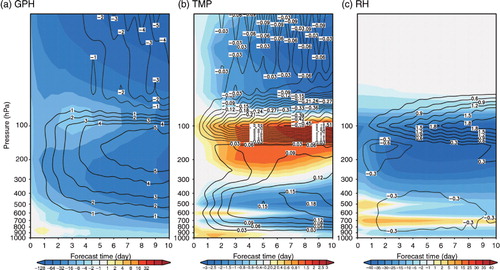
The evaluation of the hybrid coordinate is further extended for all layers to check for mean bias. Figure 6 shows a time series of vertical profiles for bias in the tropics. Compared to the ERA-Interim analysis, the SIG run generally shows a lower geopotential height for all vertical layers (Fig. 6a; shading). Moreover, it shows a cold and dry bias but has a warm temperature bias between 100 and 200 hPa (Fig. 6b and 6c; shading). The model biases are alleviated by incorporating the hybrid coordinate. The HYB run increases the low geopotential height that appeared in the SIG run (Fig. 6a; contour) and adequately corrects cold (or warm) and dry biases in temperature and relative humidity, respectively (Fig. 6b and Fig. 6c; contour). However, a sudden change in the bias correction of geopotential height through 100 hPa still exists. This issue is further discussed in the next section.

Fig. 6 Time series of the vertical profiles of the difference in (a) geopotential height, (b) temperature, and (c) relative humidity in the tropics (shading, SIG minus ERA; contour, HYB minus SIG). The 31-ensemble members initialised at 0000 UTC are averaged at each forecast time during August 2010.

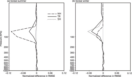
To elucidate the improvement in relative humidity, the vertical profile of the normalised difference in RMSE for the 5-d forecast is plotted in Fig. 7. Compared with that of the SIG run, the RMSE of the HYB run is distinctly reduced near 100 hPa in the Northern Hemisphere for the boreal summer (Fig. 7a) and in the Southern Hemisphere for the boreal winter (Fig. 7b). Some improvement is also discernible in the tropics near the 100 hPa level. At other levels, there is little if any difference in RMSE in all regions. Although moisture diminishes marginally with increasing layer height, the improvement is expected to notably enhance tracer advection in the upper troposphere or lower stratosphere.

Fig. 7 Vertical profile of the normalised difference in RMSE of relative humidity between the HYB and SIG runs at forecast day 5. The 31-ensemble members initialised at 0000 UTC are averaged at each forecast time during (a) August 2010 and (b) January 2011, and the verification is against the ERA Interim analysis in the northern hemisphere (dashed), tropics (solid), and southern hemisphere (dotted).

4.3. SPH versus DFS

In the SPH dynamical core, an evaluation of the hybrid sigma-pressure vertical coordinate reveals that the impact of the hybrid coordinate on forecast skill is almost the same as that in the DFS dynamical core in terms of precipitation and large-scale features. Validation scores for precipitation over the Korean peninsula do not differ much between the SIGsph and HYBsph runs (not shown). In terms of large-scale features on a medium-range time scale, Table 4 shows that the improvement in forecast skill for a 500 hPa geopotential height and temperature is discernible at forecast-day 5.

Table 4. Same as Table 3 but simulated by the SPH dynamical core. Better scores are highlighted in bold.

August 2010		January 2011
Variable	Experiment	00UTC	12UTC	00UTC	12UTC
Northern Hemisphere
SIGsph	44.7/0.816	43.1/0.829	59.0/0.863	59.1/0.864
HYBsph	44.7/0.816	43.1/0.829	58.7/0.864	59.0/0.864
Tropics
GPH	SIGsph	20.7/0.548	21.4/0.564	22.5/0.670	22.8/0.673
HYBsph	19.6/0.555	20.2/0.566	21.4/0.671	21.6/0.679
Southern Hemisphere
SIGsph	73.3/0.801	73.2/0.807	55.6/0.825	55.2/0.823
HYBsph	73.2/0.801	72.7/0.809	55.3/0.827	55.0/0.824
Northern Hemisphere
SIGsph	2.38/0.926	2.33/0.931	2.85/0.958	2.84/0.959
HYBsph	2.36/0.927	2.31/0.932	2.82/0.959	2.82/0.959
Tropics
TMP	SIGsph	2.28/0.367	2.34/0.363	1.84/0.612	1.89/0.639
HYBsph	2.15/0.377	2.22/0.370	1.76/0.615	1.79/0.644
Southern Hemisphere
SIGsph	3.11/0.955	3.07/0.957	2.66/0.957	2.60/0.959
HYBsph	3.09/0.955	3.05/0.957	2.65/0.957	2.59/0.959

Figure 8 shows the differences in geopotential height and temperature simulated by the DFS and SPH dynamical cores. On the sigma coordinate, the difference in intensity between the SIG and SIGsph runs changes rapidly through 100 hPa. The SIG run reproduces relatively low (high) geopotential heights below (above) 100 hPa (Fig. 8a). This feature is also apparent in Fig. 6a, where the contour indicates the difference between the HYB and SIG runs. In terms of temperature, the SIG run yields a cold (warm) bias below 300 hPa (near 100 hPa) compared to the SIGsph run (Fig. 8b). Moreover, the 100 hPa warm bias is gradually increased with forecast time. When the hybrid coordinate is applied, the biases near 100 hPa are clearly removed. A consistently low bias appears at geopotential heights above and below 100 hPa (Fig. 8c), and the corresponding warm bias disappears near this level (Fig. 8d).

Fig. 8 Same as Fig. 6, except for the differences in (a),(c) geopotential height and (b),(d) temperature (left) between the SIG and SIGsph runs and (right) between the HYB and HYBsph runs. Contour intervals are 1 and 0.05 K for geopotential height and temperature, respectively. Heavy and light shading indicates the positive and negative bias, respectively.

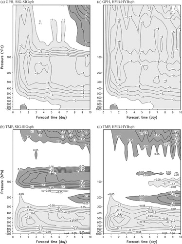
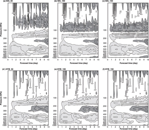
The bias of the sigma coordinate is attributed to different numerical diffusion methods between the two dynamical cores. While the strength of diffusion damping increases higher up within the SPH dynamical core, the DFS dynamical core uses an unique horizontal diffusion method which classifies diffusivity into three categories in terms of vertical layer (P2013). This is due to the fact that it would be computationally inefficient to apply different diffusion coefficients across all vertical layers since the DFS Laplacian operator requires a time-consuming tridiagonal matrix that depends on horizontal diffusion coefficients. Three diffusivities are empirically determined through comparison with the SPH dynamical core, and there is a strong transition of diffusivity at sigma layer 0.1, which corresponds to approximately 100 hPa. Another transition occurs at 0.7, at which point there occurs a smoother change in diffusivity (see P2013). In Fig. 9, the impact of the transition layer is tested with three different sigma values: 0.05, 0.1, and 0.15. The results reveal that the location of warm bias depends upon the transition layer on the sigma coordinate (Fig. 9a–Fig. 9c). This problem is adequately corrected by incorporating hybrid coordinates following isobaric levels in the upper layer. In Fig. 9d–Fig. 9f, the numerical warm bias is clearly removed, and the overall bias pattern is insensitive to the location of the strong diffusivity transition.

Fig. 9 Same as Fig. 8 but for temperature simulated by single-run on (a)–(c) sigma and (d)–(f) hybrid vertical coordinates. The DFS diffusion coefficient is rapidly changed at the sigma layers of (left) 0.05, (middle) 0.1, and (right) 0.15.

5. Concluding remarks

A hybrid sigma-pressure vertical coordinate system was newly devised for the DFS dynamical core of the GRIMs. In addition to its implementation, the system was quantitatively assessed in terms of precipitation and diagnostics at different horizontal resolutions and various time scales.

The new hybrid coordinate was successfully implemented into the DFS dynamical core, which was confirmed by the positive effect on forecast skill as compared with the terrain-following sigma coordinate. Nearly identical results were achieved using the SPH dynamical core with the hybrid coordinate. There was little difference between the DFS experiments using the sigma and hybrid coordinates in terms of heavy rainfall since precipitation is controlled mainly by dynamics in the lower half of the troposphere where the hybrid coordinate is very similar to the terrain following coordinate; however, the precipitation pattern simulated by the hybrid coordinate more closely resembled the rain-gauge and TMPA data. Improvements in traditional skill scores for medium-range forecasting were achieved using the hybrid coordinate for both the summer and winter seasons. Geopotential height was better simulated by the hybrid coordinate in the upper layer because the coordinate system gradually changes from a terrain-following layer to a pressure surface. In addition, temperature skills were improved for all regions irrespective of season. The RMSE for relative humidity was remarkably reduced near 100 hPa, especially in the Northern Hemisphere in a boreal summer. This improvement is worth noting for its ability to capture tracer advection in the upper troposphere or lower stratosphere.

For the DFS dynamical core, the hybrid coordinate adequately corrected the 100 hPa bias of the sigma coordinate caused by the rapid transition of diffusivity at sigma layer 0.1. This was achieved by numerical diffusion along a pressure surface in the upper layer of the atmosphere. This suggests that, for the DFS dynamical core, the hybrid coordinate would be more suitable and is necessary for the unique horizontal diffusion method used.

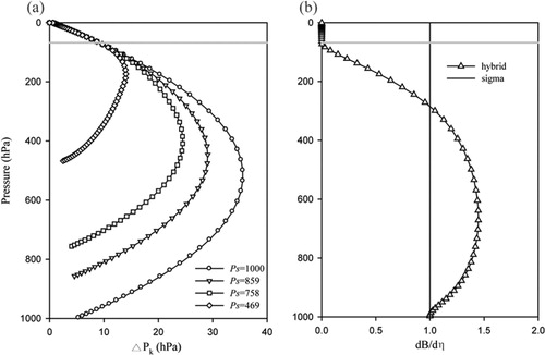
The hybrid sigma-pressure vertical coordinate is dependent on several parameters such as the reference pressure and temperature, the pressure level converted from terrain-following levels to isobaric surfaces, and the isobaric and terrain-following coefficients. These properties considerably affect the stability of semi-implicit time stepping as well as forecast skill. E2009 pointed out that thickness discontinuities at the coordinate transition layer can be fixed by adjusting the vertical derivative of the terrain-following coefficient, resulting in improved forecast skill. Fig. 10a shows that the implemented hybrid coordinate does not induce thickness discontinuities at a transition layer of 68 hPa. This is attributed to the well-regulated profile of the terrain-following coefficients seen in Fig. 10b, which is very similar to the fifth generation European Centre Hamburg Model (ECHAM5) (Roeckner et al., 2003) formulation (see Fig. 17e in E2009). E2009 also noted that, in terms of short- and medium-range forecast skill, there is no practical evidence to recommend one unique hybrid coordinate choice over another, which confirms the validity of the wide range of hybrid coordinates used in the current NWP and climate models. Hence, there remains considerable potential to improve the hybrid coordinate by revising the aforementioned properties. Additionally, the effect of the hybrid coordinate system on data assimilation and chemical transport in the stratosphere should be investigated in future studies.

Fig. 10 (a) Layer pressure thickness versus pressure at surface pressures of 1000, 859, 758, and 469 hPa, and (b) profile of derivative of terrain-following coefficient. The gray line indicates the lowest pure pressure interface level (~68 hPa).

6. Acknowledgments

This work was supported by Basic Science Research Program through the National Research Foundation of Korea (NRF) funded by the Ministry of Education, Science and Technology (2012-0000158), and by the Korea Meteorological Administration Research and Development Program under Grant CATER 2012-3084. The authors would like to acknowledge the support from KISTI supercomputing centre through the strategic support program for the supercomputing application research [No. KSC-2012-G2-02]. We also acknowledge Hyeong-Bin Cheong for discussion on the DFS dynamical core.

References

- Allen D. R , Coy L , Eckermann S. D , McCormack J. P , Manney G. L , co-authors . NOGAPS-ALPHA Simulations of the 2002 Southern hemisphere stratospheric major warming. Mon. Weather. Rev. 2006; 134: 498–518.
- Arakawa A , Lamb V. R , Chang J . Computational design of the basic dynamical process of the UCLA general circulation model. Methods in Computational Physics. 1977; Academic Press, New York. 173–265.
- Cheong H.-B . Application of double Fourier series to the shallow-water equations on a sphere. J. Comput. Phys. 2000a; 165: 261–287.
- Cheong H.-B . Double Fourier series on a sphere: applications to elliptic and vorticity equations. J. Comput. Phys. 2000b; 157: 327–349.
- Cheong H.-B . A dynamical core with double Fourier series: comparison with the spherical harmonics method. Mon. Weather. Rev. 2006; 134: 1299–1315.
- Cheong H.-B , Kwon I.-H , Goo T.-Y . Further study on the high-order double-Fourier-series spectral filtering on a sphere. J. Comput. Phys. 2004; 193: 180–197.
- Cheong H.-B , Kwon I.-H , Goo T.-Y , Lee M.-J . High-order harmonic spectral filter with the double Fourier series on a sphere. J. Comput. Phys. 2002; 177: 313–335.
- Collins W. D , Rasch P. J , Boville B. A , Hack J. J , McCaa J. R , co-authors . Description of the NCAR Community Atmopphere Model (CAM 3.0).
- Covey C , AchutaRao K. M , Cubasch U , Jones P , Lambert S. J , co-authors . An overview of results from the Coupled Model Intercomparison Project. Global. Planet. Change. 2003; 37: 103–133.
- Dai A . Precipitation characteristics in eighteen coupled climate models. J. Clim. 2006; 19: 4605–4630.
- Dee D. P , Uppala S. M , Simmons A. J , Berrisford P , Poli P , co-authors . The ERA-Interim reanalysis: configuration and performance of the data assimilation system. Q. J. Roy. Meteorol. Soc. 2011; 137: 553–597.
- Eckermann S . Hybrid σ–p coordinate choices for a global model. Mon. Weather. Rev. 2009; 137: 224–245.
- Hong S.-Y , Park H , Cheong H.-B , Kim J.-E. E , Koo M.-S , co-authors . The global/regional integrated model system (GRIMs). Asia-Pacific. J. Atmos. Sci. 2013; 49(2): 219–243.
- Huffman G. J , Bolvin D. T , Nelkin E. J , Wolff D. B , Adler R. F , co-authors . The TRMM multisatellite precipitation analysis (TMPA): quasi-global, multiyear, combined-sensor precipitation estimates at fine scales. J. Hydrometeorol. 2007; 8: 38–55.
- Janjic Z. I . The NCEP WRF core. Proceedings of the 20th Conference on Weather Analysis and Forecasting/16th Conference on Numerical Weather Prediction. 2004. Seattle, Washington, 10–25 January, Amer. Meteor. Soc., 21 p. Online at: http://ams.confex.com/ams/pdfpapers/70036.pdf .
- Juang H.-M. H . A reduced spectral transform for the NCEP seasonal forecast global spectral atmospheric model. Mon. Weather. Rev. 2004; 132: 1019–1035.
- Juang H.-M. H , Hong S.-Y , Kanamitsu M . The NCEP regional spectral model: an update. Bull. Ame Meteorol. Soc. 1997; 78: 2125–2143.
- Kanamitsu M , Ebisuzaki W , Woollen J , Yang S.-K , Hnilo J. J , co-authors . NCEP–DOE AMIP-II reanalysis (R-2). Bull. Am. Meteorol. Soc. 2002a; 83: 1631–1643.
- Kanamitsu M , Kumar A , Juang H.-M. H , Schemm J.-K , Wang W , co-authors . NCEP dynamical seasonal forecast system 2000. Bul. Am. Meteorol. Soc. 2002b; 83: 1019–1037.
- Koo M.-S , Hong S.-Y , Kim J . An evaluation of the tropical rainfall measuring mission (TRMM) multi-satellite precipitation analysis (TMPA) data over south Korea. Asia-Pacific. J. Atmos. Sci. 2009; 45: 265–282.
- Layton A. T , Spotz W. F . A semi-Lagrangian double Fourier method for the shallow water equations on the sphere. J. Comput. Phys. 2003; 189: 180–196.
- Pacanowski R. C , Griffies S. M . MOM 3.0 manual. NOAA/GFDL. 1998. Oneline at: http://www.gfdl.noaa.gov/~smg/MOM/web/guide_parent/guide_parent.html .
- Park H , Hong S.-Y , Cheong H.-B , Koo M.-S . A double Fourier series (DFS) dynamic core in a global atmospheric model with full physics. Mon. Weather. Rev. 2013. Online at: http://journals.ametsoc.org/action/showCitFormats?doi=10.1175%2FMWR-D-12-00270.1 .
- Phillips N. A . A coordinate system having some special advantages for numerical forecasting. J. Meteorol. 1957; 14: 184–185.
- Reynolds R. W , Smith T. M . Improved global sea surface temperature analyses using optimum interpolation. J. Clim. 1994; 7: 929–948.
- Roeckner E , Bäuml G , Bonaventura L , Brokopf R , Esch M , co-authors . The Atmospheric General Circulation Model ECHAM5. Part I: Model Description.
- Schär C , Leuenberger D , Fuhrer O , Lüthi D , Girard C . A new terrain-following vertical coordinate formulation for atmospheric prediction models. Mon. Weather. Rev. 2002; 130: 2459–2480.
- Sela J. G . The Implementation of the Sigma Pressure Hybrid Coordinate into the GFS.
- Seol K.-H , Hong S.-Y . Relationship between the Tibetan Snow in Spring and the East Asian Summer Monsoon in 2003: a global and regional modeling study. J. Clim. 2009; 22: 2095–2110.
- Simmons A. J , Burridge D. M . An energy and angular-momentum conserving vertical finite-difference scheme and hybrid vertical coordinates. Mon. Weather. Rev. 1981; 109: 758–766.
- Simmons A. J , Strüfing R . Numerical forecasts of stratospheric warming events using a model with a hybrid vertical coordinate. Q. J. Roy. Meteorol. Soc. 1983; 109: 81–111.
- Taylor M , Tribbia J , Iskandarani M . The spectral element method for the shallow water equations on the sphere. J. Comput. Phys. 1997; 130: 92–108.
- Tygert M . Fast algorithms for spherical harmonic expansions, III. J. Comput. Phys. 2010; 229: 6181–6192.
- White P. W . IFS Documentation. Part III: Dynamics and Numerical Procedures (Cy37r2). 2011; ECMWF, Reading, UK,: Meteorological Bulletins. 29.
- Williamson D. L . The evolution of dynamical cores for global atmospheric models. J. Meteorol. Soc. Japan. 2007; 85B: 241–269.
- Williamson D. L , Drake J. B , Hack J. J , Jakob R , Swarztrauber P. N . A standard test set for numerical approximations to the shallow water equations in spherical geometry. J. Comput. Phys. 1992; 102: 211–224.
- WMO. Manual on the Global Data-Processing and Forecasting system, Volume I - Global Aspects. 2012; Geneva, Switzerland: World Meteorological Organization. II. 7-36 - II. 7-38. Online at: http://www.wmo.int/pages/prog/www/DPFS/documents/485_Vol_I_en_colour.pdf .
- Xie P , Arkin P. A . Global precipitation: a 17-year monthly analysis based on gauge observations, satellite estimates, and numerical model outputs. Bull. Am. Meteorol. Soc. 1997; 78: 2539–2558.
- Zängl G . A generalised sigma-coordinate system for the MM5. Mon. Weather. Rev. 2003; 131: 2875–2884.