Ensemble data assimilation with an adjusted forecast spread

Abstract

Ensemble data assimilation typically evolves an ensemble of model states whose spread is intended to represent the algorithm's uncertainty about the state of the physical system that produces the data. The analysis phase treats the forecast ensemble as a random sample from a background distribution, and it transforms the ensemble according to the background and observation error statistics to provide an appropriate sample for the next forecast phase. We find that in the presence of model nonlinearity and model error, it can be fruitful to rescale the ensemble spread prior to the forecast and then reverse this rescaling after the forecast. We call this approach forecast spread adjustment, which we discuss and test in this article using an ensemble Kalman filter and a 2005 model due to Lorenz. We argue that forecast spread adjustment provides a tunable parameter, that is, complementary to covariance inflation, which cumulatively increases ensemble spread to compensate for underestimation of uncertainty. We also show that as the adjustment parameter approaches zero, the filter approaches the extended Kalman filter if the ensemble size is sufficiently large. We find that varying the adjustment parameter can significantly reduce analysis and forecast errors in some cases. We evaluate how the improvement provided by forecast spread adjustment depends on ensemble size, observation error and model error. Our results indicate that the technique is most effective for small ensembles, small observation error and large model error, though the effectiveness depends significantly on the nature of the model error.

• ensemble
• Kalman filter
• data assimilation
• forecast spread
• covariance inflation

1. Introduction

Data assimilation is used, for example, to determine initial conditions for weather forecasts from the information provided by atmospheric observations. Combining a prior weather forecast with observations and taking into account the uncertainties of each, data assimilation attempts to provide an optimal estimate for the current state of the atmosphere. Modifying the forecast to better fit to the observations is called the analysis phase of data assimilation. The resulting estimate, also called the analysis, is then evolved during the forecast phase.

In data assimilation, the observation uncertainty is typically characterised as additive errors distributed according to a known Gaussian distribution whose covariance is constant in time. Forecast errors are often treated as Gaussian too, but the actual forecast error covariance changes in time and can be difficult to estimate. Ensemble data assimilation uses an ensemble of forecasts to provide a statistical sampling of the plausible atmospheric states, estimating the forecast error covariance through sample statistics. Ensemble Kalman filters (EnKFs) fit the ensemble mean to the observations and provide a collection of plausible estimates (the ensemble) to represent the remaining uncertainty (Evensen, 1994; Burgers et al., 1998; Houtekamer and Mitchell, 1998; Anderson and Anderson, 1999; Bishop et al., 2001; Ott et al., 2004; Wang et al., 2004). Propagating this analysis ensemble provides the sample mean and covariance for the next assimilation cycle.

The Kalman filter (Kalman, 1960) is optimal for linear models with Gaussian errors. Algorithms that extend the Kalman filter to nonlinear models, including EnKFs among others, are suboptimal and can diverge even if there is no model error (Jazwinski, 1970; Anderson and Anderson, 1999). One reason is that model nonlinearity causes EnKFs to underestimate the forecast error covariance relative to the uncertainty in the initial conditions (Whitaker and Hamill, 2002). Insufficient ensemble covariance can also be caused by unquantified errors in the model and observations. One common way to compensate for covariance underestimation is to inflate the forecast error covariance by a multiplicative factor larger than one during each analysis phase (Anderson and Anderson, 1999; Whitaker and Hamill, 2002; Miyoshi, 2011). Other ways to compensate for the underestimation include additive inflation (Houtekamer and Mitchell, 2005; Whitaker et al., 2007), relaxation-to-prior-perturbations (Zhang et al., 2004) and relaxation-to-prior-spread (Whitaker and Hamill, 2012).

Typically, the ensemble is propagated with spread representative of the approximate covariance as described above. However, the ensemble covariance is only utilised during the analysis phase of data assimilation. In this article, we investigate the potential advantages of evolving an ensemble whose spread is not commensurate with the approximate covariance, by rescaling the ensemble perturbations by a factor η before the forecast phase and rescaling them by 1/η after the forecast phase. We call this technique forecast spread adjustment (FSA), and we remark that it has no net effect with a linear model.

For a nonlinear model, FSA affects the ensemble that provides the input (‘background’) for the analysis phase in three ways: changing its mean; changing the space spanned by the perturbations from the mean; and to a lesser extent, changing the size of these perturbations (the size is affected directly by covariance inflation). In an EnKF, the analysis phase adjusts the ensemble mean within the space spanned by the perturbations; FSA with η>1 may improve the ability of this space to capture the truth by increasing the chances that the forecast ensemble surrounds the truth. (On the other hand, η should not be so large than none of the ensemble members are near the truth.) Further, FSA may help overcome the rank deficiency of a small ensemble by accentuating model nonlinearities that can introduce new directions of uncertainty into the space spanned by the perturbations (and thus into the background covariance used in the analysis). We argue that FSA also has the potential to improve the forecast mean, based on the advantage sometimes observed in ensemble prediction of the mean of an ensemble forecast versus the forecast of the ensemble mean (see e.g. Buizza et al., 2005). If the mean of the forecast from an unscaled ensemble (η=1) is more accurate (on average) than the forecast of the mean (corresponding to η→0), then the mean of the forecast from an ensemble scaled by η≠1 may be better still.

FSA allows us to relate some aspects of data assimilation that were previously considered independently.

• As we will later show, for a linear observation operator FSA has the same long-term effect on the analysis means as rescaling the observation error covariance (e.g. Stroud and Bengtsson, 2007) by η ², but it results in a different (and in the scenarios we considered, more appropriate) analysis covariance.

• Multiplicative covariance inflation, described above, is applied sometimes by rescaling the forecast (background) ensemble perturbations and sometimes by rescaling the analysis ensemble perturbations (e.g. Houtekamer and Mitchell, 2005; Bonavita et al., 2008; Kleist, 2012); when using FSA in addition to inflation, both ensembles are rescaled by amounts that can be varied independently. From this point of view our approach treats forecast perturbation rescaling and analysis perturbation rescaling as techniques that can be used in tandem, as opposed to alternate versions of the same technique. We also consider the possibility of, for example, analysis perturbation inflation coupled with deflating the forecast perturbations by a lesser amount.

• The limit η→0 discussed above also corresponds to evolving the ensemble covariance according to the linear approximation about the mean, as in the extended Kalman filter (XKF; e.g. Jazwinski, 1970; Evensen, 1992).

In Section 2, we describe various data assimilation algorithms based on the Kalman filter, specifically the XKF and the ensemble Kalman filters, ETKF (Bishop et al., 2001; Wang et al., 2004) and LETKF (Hunt et al., 2007). In Subsection 3.1, we describe FSA. We compare FSA to alternative formulations that can produce the same analysis means, specifically: inflating the observation error covariance (Subsection 3.2) and inflating the analysis error covariance in addition to or instead of the background (forecast) error covariance (Subsection 3.3). The main difference between these approaches is that inflating the observation error covariance results in a larger background and analysis error covariance than FSA. Subsection 3.4 compares the ensemble transform Kalman filter (ETKF) and the XKF and discusses how FSA can transition from the XKF to the ETKF and beyond. In Subsection 4.1 we describe the Lorenz (2005) Model II used for our experiments, and in Subsection 4.2 we describe our experiments. In Subsection 4.3 we describe how we tuned the FSA parameter η, along with the multiplicative covariance inflation factor, in order to minimise analysis errors. We also discuss the possibility of adaptively tuning both parameters with techniques similar to Li et al. (2009). Subsection 4.4 depicts and discusses the results of our experiments. We summarise our findings and state our conclusions in Section 5.

2. Kalman filters

The Kalman filter is an optimal algorithm for data assimilation with a linear model with Gaussian errors. A Kalman filter can be described by the cycle of forecasting the previous analysis (optimal estimate) to get the background (forecast) and generating a new analysis by updating the background to more closely match the observations. Thus, we describe the Kalman filter in terms of two phases: the forecast phase and the analysis phase. Most data assimilation algorithms used for weather prediction (including variational methods and EnKFs) have the same statistical basis as the Kalman filter.

The analysis state according to the Kalman filter is given by1 2 where K is the Kalman gain matrix, x ^a is the analysis state, x ^b is the forecast or background state, P ^b is the background error covariance, R ^o is the observation error covariance, y ^o is the vector of observations, h is the observation operator that transforms model space into observation space, and H is the matrix that linearises h about x ^b. The error covariance of the analysis state x ^a is given by3 Having determined x ^a and P ^a at a certain time t, the forecast phase evolves these to the background state and its error covariance at time t ⁺>t. Specifically, in the forecast phase from time t to time t ⁺, the model M evolves the analysis state at time t to the background state at time t ⁺. The forecast phase is given by4 5 where Q is a covariance matrix representing model errors, which, like observation errors, are assumed to be Gaussian.

Nonlinear extensions of the Kalman filter generally use eq. (1)–(3) with minor modifications and differ primarily in how they evolve the estimated state and covariance. For EnKFs, a common alternative to the model error term in (5) is to inflate by a multiplicative factor ρ (Anderson and Anderson, 1999). Such multiplicative inflation can be helpful even if there is no model error, since a nonlinear model tends to cause the ensemble to underestimate the background error covariance (Whitaker and Hamill, 2002).

2.1. Ensemble Kalman filters (EnKFs)

In this section, we discuss the class of data assimilation techniques known as the EnKFs. In the ensemble techniques, rather than evolving the covariance directly as done in the Kalman filter and the XKF, an ensemble is chosen to represent a statistical sampling of a Gaussian background distribution, with the sample mean of the background ensemble approximating the background state x ^b in eq. (1). The subscript i here refers to the index of the ensemble member, and the ensemble has k members in total. All members of the ensemble estimate the background at the same time.

Each ensemble member can be expressed as a sum of the mean and a perturbation . Letting and be the matrices with columns and _, respectively, we write6 where by adding a vector and a matrix we mean adding the vector to each column of the matrix. The columns of X ^b represent the ensemble of background perturbations, constructed as departures from the mean.

The background error covariance is computed from the background ensemble according to sample statistics, namely7 where ρ is the multiplicative covariance inflation factor (discussed in Subsection 3.3).

We use a corresponding notation for the analysis ensemble with mean and perturbations X ^a. EnKFs are designed to satisfy the Kalman filter eq. (1)–(5) with x ^b and x ^a replaced by and . Mimicking the background, the analysis ensemble perturbations must correspond to a square root of the reduced-rank analysis error covariance matrix in eq. (3), that is,8 Different EnKFs select different solutions X ^a to this equation. Finally, in all EnKFs, the ensemble members are propagated independently. For a deterministic (possibly nonlinear) forecast model M, which propagates a model state from time t to time t ⁺, the background ensemble members at time t ⁺ are given by9

2.1.1. ETKF

We tested ensemble data assimilation with FSA on the ETKF (Bishop et al., 2001; Wang et al., 2004) and the Local Ensemble Transform Kalman Filter (LETKF) (Ott et al., 2004; Hunt et al., 2007). We implemented both methods according to the formulation in Hunt et al. (2007) (see Subsection 2.1.2 for the relationship between LETKF and ETKF). For speedy computation, in these algorithms the analysis phase of the Kalman filter is performed in the space of the observations, with the background ensemble transformed into that space for comparison.

In the ETKF, the analysis mean is given by10 11 where h is the (possibly nonlinear) observation operator, and Y ^b are the background perturbations in observation space derived by transferring the ensemble to observation space and subtracting the mean For a linear observation operator, the ETKF analysis mean computed in eq. (10) equals the Kalman filter analysis estimate x ^a of eq. (1) assuming and [eq. (7)].

The ETKF analysis perturbations are given by12 where the exponent represents taking the symmetric square root. These perturbations differ from the background perturbations as little as possible while still remaining a square root of P ^a (Ott et al., 2004). For a full discussion of the equivalence and relationship between (10)–(12) and (1)–(3), see Hunt et al. (2007).

2.1.2. LETKF

Essentially, the LETKF performs an ETKF analysis at every model grid point, excluding distant observations from the analysis. At each grid point, it computes and , truncating y ^o and R ^o to include only the observations within a certain distance from the grid point. The LETKF computes the local analysis for each grid point from the ETKF analysis eq. (10)–(12) and restricts the resulting analysis to that grid point alone. Observation localisation is motivated and explored in (Houtekamer and Mitchell, 1998; Ott et al., 2004; Hunt et al., 2007; Greybush et al., 2011). We provide a limited motivation here.

One problem with estimating P ^b [eq. (7)] from an ensemble is that sampling error can introduce artificial correlations between the background error at distant grid points. As the analysis increment in eq. (10) is computed in observation space, it is possible to eliminate these spurious correlations (along with any real correlations) for the analysis at a particular model grid point by truncating the observation space beyond a specified distance from the grid point.

Other methods of localisation (e.g. Whitaker and Hamill, 2002; Bishop and Hodyss, 2009) modify the background error covariance directly. For all these approaches, localisation is found to greatly reduce the number of ensemble members needed to produce reasonable analyses for models with large spatial domains.

2.2. Extended Kalman filter (XKF)

In the XKF (see e.g. Jazwinski, 1970), the model evolves the analysis x ^a as in eq. (4) to determine the subsequent background , and the background error covariance is determined from P ^a by linearising the model at x ^a. For more information on the XKF and how it compares to EnKFs, see Evensen (2003) and Kalnay (2003).

Like the Kalman filter, the XKF is usually formulated with an additive model error term that increases the background covariance. However, for ease of comparison to the ETKF, our implementation of the XKF uses multiplicative inflation instead of additive inflation.

One major difficulty with the XKF is the computational cost of evolving the covariance matrix (Evensen, 1994; Burgers et al., 1998; Kalnay, 2003). This makes the model unfeasible for high-dimensional models in a realistic setting. However, when using simple test models such as the Lorenz (2005) Model II, the XKF can be compared to other data assimilation techniques.

Another potential drawback of the XKF is its linear approximation when evolving the covariance (Evensen, 2003). As we find in our experiments, this can be disadvantageous compared to the nonlinear evolution of both mean and covariance provided by an ensemble.

3. Methodology and theory

In this section, we formally describe the method of FSA for EnKFs. One way of implementing the FSA is to multiply the analysis perturbations by η prior to forecasting and, after the forecast, multiply the forecast perturbations by (Subsection 3.1). This is only has an effect when the model is nonlinear. Other authors (e.g. Stroud and Bengtsson, 2007) have found benefits from multiplicative observation error covariance inflation, motivated by observation errors other than measurement error. In Subsection 3.2, we show that FSA by η is closely related to inflating R ^o by η ²; both methods yield similar analysis accuracies after spin-up, but they quantify the analysis covariance differently. Thus, FSA should improve analysis accuracy in the same situations that R ^o inflation does; the method that yields a more appropriate analysis covariance should depends on whether the improvement is more due to model error and nonlinearity (the motivation for FSA) or due to unquantified observation errors (the motivation for R ^o inflation). The FSA motivation applies better to our numerical experiments, in which the observations lie on the model grid points, and the observation operator and observation error covariance are known exactly.

3.1. Ensemble data assimilation with FSA

This section describes the technique of expanding (or shrinking if η<1) the ensemble perturbations for the forecast and shrinking (or expanding) the ensemble for the analysis. After (1) finding the analysis through any ensemble data assimilation technique, the background perturbations in the next cycle are obtained by: (2) multiplying the analysis perturbations by η, (3) evolving the adjusted analysis ensemble and (4) multiplying the forecast perturbations by .

Mathematically, this can be expressed with a matrix transformation S corresponding to an expansion factor η:13 where14 15 The model integration of the matrix in eq. (13) refers to forecasting each ensemble member (column of ) separately, that is,

For an ensemble of size k, each column of the [k×k] matrix 1 _k×k right transforms an ensemble into its row sum so that . Thus, right multiplication by S transforms each ensemble member into a weighted average of itself (prior to adjustment) and the mean of the ensemble:16 Viewed another way, right multiplication by S scales the ensemble perturbations by η, producing a new ensemble with the same mean:17 Notice that:18 so S ⁻¹ effectively rescales ensemble perturbations by η ⁻¹. We call an analysis expansion and a forecast re-contraction forecast spread adjustment (abbreviated FSA). We remark that for a linear model, the S and S ⁻¹ in eq. (13) cancel each other out, so that FSA with η≠1 does not change the result from that of a forecast without FSA.

The full Kalman filter cycle from to with the forecast phase described by eq. (13) is given in the following algorithm. (1) Perform analysis on to find . (2) Left multiply by S to scale the perturbations X ^a by a factor of η, (i.e. X ^a,f=ηX ^a)19 (3) Evolve each member of the resulting ensemble: 20 (4) Left multiply by S ⁻¹ to rescale the perturbations of the evolved ensemble by 21 Here and elsewhere, and refer to the ensemble during the forecast phase. We abbreviate the ETKF with FSA and the LETKF with FSA (via a scaling factor of η) as the ηETKF and the ηLETKF respectively.

We remark that when η=1, ensemble data assimilation with FSA reduces to standard ensemble data assimilation. Furthermore, if the model is linear, FSA has no net effect. When the model is nonlinear, FSA can affect both the background mean and the background covariance. Since multiplicative inflation is already affecting the covariance, the additional impact of FSA may be mainly due to its effect on the mean.

3.2. Relation to inflation of the observation error covariance

Some authors have recommended scaling the reported observation error covariance, assuming that it is misrepresented (e.g. Stroud and Bengtsson, 2007; Li et al., 2009). As we will show below, inflating the observation error covariance is closely related to FSA, and thus in many cases both approaches can improve the analyses. Indeed, if the observation operator h is linear then we will show that both approaches, if initialised with the same forecast ensemble, will produce the same analysis means. Having the same forecast ensembles implies that during the analysis phase, the two approaches will use different ensemble perturbations (related by a factor of η) and hence different covariances.

3.2.1. ηETKF without R^o inflation

Let be the initial background ensemble. In this case, we perform ensemble data assimilation with FSA to find . The ηETKF analysis ensemble is given by eq. (10)–(12) repeated here for convenience22 23 24 The next background ensemble is given by eq. (13)25

3.2.2. ETKF with R^o inflated to η²R^o

Let the initial background ensemble be and assume that . Based on eq. (21), we also write . It follows that this implies the additional equivalences and . We perform standard ensemble data assimilation to find assuming an observation error covariance of η² times its value in Case 3.2.1. We compare with and .

In this case (3.2.2), the analysis ensemble is given by eq. (10)–(12), with R ^o₂ =η ² R ^o replacing R ^o. After algebraic manipulation, these equations are26 27 28 Substituting X ^b₂ =ηX ^b and assuming a linear observation operator so that Y ^b₂ =ηY ^b, we find that29 30 31 Thus, . And from eq. (19), ; thus, the ensembles are identical during evolution.

The next background ensemble is given by32 Comparing this to eq. (25), we see that ; therefore . In other words, the means remain the same and the perturbations maintain the same ratio.

We remark that although both cases evolve the same ensemble, the error covariances in the two cases differ by the factor η ². This is demonstrated in Fig. 1.

Fig. 1 (a) Data assimilation with a forecast spread adjustment of η. (b) Standard data assimilation with R ^o inflated by η ². The two data assimilation cycles depicted above are initialised during the forecast phase, that is, .

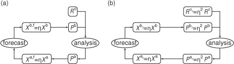
From the correspondence described above, which assumes that the two filters are initialised with the same forecast ensemble, it follows that they will produce similar means in the long term even if they are initialised differently, as long as the filters themselves are insensitive in the long term to how they are initialised.

3.3. Which to inflate, P^a or P^b?

As discussed in the beginning of Section 2, due to nonlinearity and model error ensemble data assimilation tends to underestimate the evolved error covariance. Multiplicative inflation of the background error covariance was proposed (Anderson and Anderson, 1999; Whitaker and Hamill, 2002) to compensate. For practical reasons, some implementations (e.g. Houtekamer and Mitchell, 2005; Bonavita et al., 2008; Kleist, 2012) inflate the analysis ensemble rather than the background ensemble; this amounts to inflating before the forecast rather than after. With FSA, it no longer becomes a question of inflating one or the other; instead FSA provides a continuum connecting P ^b multiplicative inflation and P ^a multiplicative inflation.

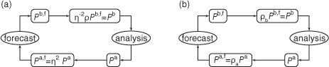
Consider the standard data assimilation cycle as it applies to P ^a and P ^b with multiplicative analysis and background covariance inflation of ρ _a and ρ _b respectively (Fig. 2a), and assume as in the previous section that the observation operator h is linear. Following the algorithms given in Hunt et al. (2007), in our implementation of the ηETKF, we effectively inflate the background error covariance (Fig. 2b). By setting η=√ρ, we transform a data assimilation algorithm that inflates the background error covariance P ^b into a data assimilation algorithm that inflates the analysis error covariance P ^a. Furthermore, this comparison demonstrates that ensemble data assimilation with an adjusted forecast spread and with multiplicative background error covariance inflation can be alternatively interpreted as standard data assimilation, inflating both the background and analysis error covariances. In particular, adjusting the forecast spread by η and inflating the background error covariance by ρ is equivalent to inflating the background error covariance by ρ _b=ρ/η ² and inflating the analysis error covariance by ρ _a=η ², provided the observation operator h is linear.

Fig. 2 (a) The data assimilation cycle on P ^b and P ^a including a forecast spread adjustment of η and inflation of P ^b with ρ. (b) The data assimilation cycle on P ^b and P ^a including inflation of P ^b with ρ _b and inflation of P ^a with ρ _a.

Houtekamer and Mitchell (2005), using additive rather than multiplicative inflation, observed improved results by inflating the analysis ensemble rather than the background ensemble. They suggest that the advantage may be due to allowing the model to evolve and amplify the perturbations that compensate for errors in the analysis as well as model errors. Our results indicate that, in some cases, there is a further advantage to using values of η that are significantly larger than √ρ, that is, over-inflating the analysis perturbations (ρ _a>ρ) and deflating the background perturbations by a lesser amount ().

3.4. Comparison to the XKF

The ETKF (Bishop et al., 2001; Wang et al., 2004) and the XKF (Jazwinski, 1970; Evensen, 1992) are similar in that they both evolve the covariance matrix in time. The XKF evolves the best estimate along with its error covariance. The ETKF evolves a surrounding ensemble which approximates the error covariance and does not explicitly evolve the best estimate, which is the mean of the ensemble.

Previous articles, for example, Burgers et al. (1998), demonstrate the equivalence between the analysis phases of the XKF and the EnKF, provided the ensemble is sufficiently large. However, this equivalence does not continue into the forecast phase. Starting from the same analysis state and the same analysis error covariance , the XKF and the EnKF will evolve different states with different error covariances .

Varying the ensemble spread changes the evolved ensemble in a nonlinear fashion, affecting the mean and perturbations (in both magnitude and direction). In the limit as η→0, the ensemble perturbations become infinitesimal and the forecast evolves the ensemble mean and the perturbations evolve according to the tangent linear model. If the ensemble is large enough that the perturbations span the model space, then a full-rank covariance is evolved according to the tangent linear model, just as in the XKF. Therefore, for a sufficiently large ensemble, the ηETKF should approach the XKF as η tends to zero; otherwise, it approaches a reduced-rank XKF. Furthermore, when η=1, the ηETKF is the standard ETKF. Thus, for intermediate values of η, the ηETKF can be considered a hybrid of the XKF and the ETKF.

In the scenarios we explored where tuning η was especially effective, η tuned to values greater than one, enhancing the advantages of the EnKF over the XKF.

4. Experiments and results

Our experiments are observed system simulation experiments (OSSEs). In OSSEs, we evolve a truth with the model, adding error at a limited number of points to simulate observations. Treating the truth as unknown, we use data assimilation to estimate it. Comparing the analysis to the truth, we estimate the accuracy of the data assimilation techniques being tested. Thus, we can evaluate and compare the accuracy of data assimilation techniques. We assessed accuracy via the root mean square error (RMSE) difference between the analysis mean and the truth evaluated at every grid point.

4.1. Models

We tested FSA on the Lorenz (2005) Model II with a smoothing parameter of K=2 [smoothing the Lorenz 96 model (Lorenz, 1996; Lorenz and Emanuel, 1998) over twice as many grid points]. For a forcing constant F and smoothing parameter K, the model state at grid point j is evolved according to33 where refers to averaging x _j , the model state at grid point j, with the model state at nearby grid points.

When K=2, the averaging includes only the grid point itself and the immediately adjacent grid points namely:34 Note that the avg function is applied to () by

Model II is evolved on a circular grid, in our experiments a circular grid with 60 grid points. We evolved the forecasts according to the Runge-Kutta fourth order method over a time step size of δt=0.05, performing an analysis every time step. Lorenz and Emanuel (1998) and Lorenz (2005) considered the time interval of 0.05 to correspond roughly to 6 hours of weather.

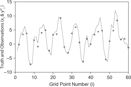
To generate the observations, we evolved the truth with a forcing constant of F ^t=12 and added independent Gaussian errors with mean 0 and standard deviation σ at every other grid point. Thus at each time step, we have 30 observations, evenly spaced among the 60 grid points, with known error covariance R ^o=σ² I _30×30. Fig. 3 gives a snapshot of these observations for σ=1 along with the truth.

Fig. 3 Sample Model II output with observations for 60 grid points, half of which are observed (*), observation error σ=1, smoothing parameter K=2 and forcing constant F=12.

4.2. Experimental design

We explored the effectiveness of tuning η in various scenarios with the LETKF. Our default parameters for data assimilation are: an observation error σ=1, an ensemble of k=10 members and a forcing constant of F=14 for the ensemble forecast to simulate model error. In all cases, we use a localisation radius of 3 grid points, that is, 3–4 observations in a local region.

Keeping the other two parameters constant at their default value, we varied the observation error, the ensemble size and the forcing constant. For instance, we varied σ=, 1, 2, keeping k=10 and F=14. We tested ensemble sizes of 5, 10, 20 and 40. We varied the forcing constant from F=9 to F=15.

In each experiment, we tuned ρ for η=1 and plotted the analysis RMSE for different values of η:35 where is the truth at time is the analysis ensemble mean at time t _i, and rms is the root mean square function over the 60 grid points; that is, the RMSE is the time averaged root mean square difference between the analysis mean and the truth. (In some cases we also computed and plotted the background RMSE, defined similarly.) In each case, we compared the minimum RMSE among the various values of η tested to the RMSE when η=1 and plotted the percent improvement36 We also tested how the ηETKF compares to the XKF for large ensembles and small η. Specifically, we tested the ηETKF for η=1, , , and 10⁻⁶ and ensembles of size k=40, 60 and 80. For η=10⁻⁶ and k=80 we expect the RMSE from the ηETKF to be very similar to the RMSE from the XKF.

4.3. Tuning η and ρ

Recall that varying η does not affect the results in the linear setting. Thus, linear theory cannot predict how the results will depend upon η in the nonlinear setting. Hence, we tune η to get the lowest RMSE during data assimilation. Similarly, we also tune the multiplicative covariance inflation factor ρ. Fig. 4 depicts the ensemble spread during both the forecast phase (red) and the analysis phase (blue) as a function of η. We define the ensemble spread by37 where N=60 is the length of the circular grid and is an N×N matrix approximating the error covariance as described in eq. (7) and (8). When η=1, the ensemble spread [eq. (37)] is intended to estimate the actual RMSE [eq. (35)]. As demonstrated in Fig. 4, when η≠1, the ensemble spread only estimates the actual RMSE during the analysis phase. In other words, the FSA parameter η only strongly affects the ensemble spread during the forecast phase (red). During the analysis phase (blue), the ensemble spread does not vary significantly with η. The minimum of the solid grey curve corresponds to the tuned value of η, which for our default parameters is η=2.5.

Fig. 4 Tuning η (grey) and the effect of η on ensemble spread during the forecast phase (red) and analysis phase (blue) for our default parameters: k=10, F=14 (F ^t=12), σ=1. Comparison of the ensemble spread during the analysis phase (blue) to the actual RMSE for various values of η (grey). The solid grey curve shows that η tunes to 2.5. We tuned η using the tuned value of ρ for η=1.

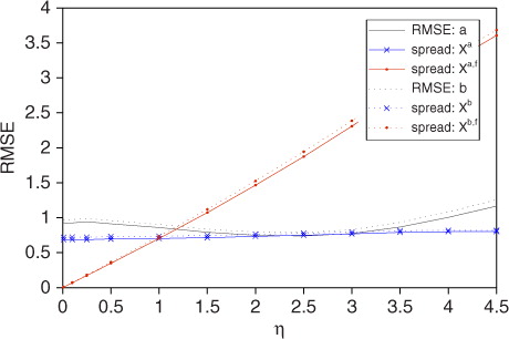
Recall (Subsection 3.2) that with observation error covariance inflation, the analysis perturbations X ^a₂ are the same as the perturbations X ^a,f for the FSA. Thus, in this scenario, according to Fig. 4, when η is tuned to a value different to one, the ensemble spread X ^a for FSA corresponds much better to the actual analysis errors than the spread X ^a₂ for observation error covariance inflation.

Figure 5 (black) demonstrates that multiplicative background error covariance inflation by ρ (Anderson and Anderson, 1999; Whitaker and Hamill, 2002) carries through to both phases of data assimilation. We remark that in this example ρ tunes to 1.20 (grey), even though the ensemble is underdispersive (the spread is lower than the RMSE). However, in this case (Fig. 4) we find that tuning η as well as ρ decreases the error to be commensurate with the ensemble spread. To tune ρ in our LETKF experiments we let η=1 and tested values of ρ differing by 0.01, choosing the value of ρ associated with the lowest analysis RMSE. The tuned values of ρ for the different cases are described in Table 1. When comparing the ηETKF to the XKF, we tuned ρ=1.29 for our XKF experiment and used that ρ for our ηETKF experiments as well.

Fig. 5 Tuning ρ and the effect of ρ on ensemble spread for our default parameters with η=1. The dotted lines correspond to the background and the solid lines correspond to the analysis. The spread is indicated in black and the RMSE in grey.

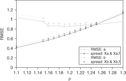
Table 1. Tuned values of ρ for LETKF with various parameters

k	F	σ	ρ
Default parameters	10	14	1	1.20
Vary k	5	14	1	1.20
10	14	1	1.20
20	14	1	1.17
40	14	1	1.15
Vary F	10	9	1	1.19
10	10	1	1.17
10	11	1	1.13
10	12	1	1.06
10	13	1	1.13
10	14	1	1.20
10	15	1	1.22
Vary σ	10	14	0.5	1.25
10	14	1	1.20
10	14	2	1.14

These values of ρ are used for the corresponding η sensitivity experiments shown in the results, although the tuning is done when η=1.

In our experiments, we determined the optimal values of ρ and η through tuning. However, there are methods that adaptively determine the values of ρ (Anderson, 2007; Li et al., 2009; Miyoshi, 2011). In particular, Li et al. (2009) simultaneously estimate values for a background error covariance inflation factor and for an observation error covariance inflation factor. When determining the analysis mean, these two parameters are equivalent in some sense to ρ and η (see Subsection 3.2). Thus, the adaptive techniques explored by Li et al. (2009) could potentially be applied to simultaneous adaptive estimation of ρ and η. On the other hand, some adjustment may be necessary if η is mainly compensating for the nonlinearity and model bias as opposed to a misspecification of the observation error covariance.

4.4. Results

Our results are given graphically as both η versus RMSE; as well as k (ensemble size), F (forcing constant) and σ (observation error) versus percent improvement in the RMSE. The RMSEs are generally accurate to the hundredth place (±0.01); the RMSEs from five independent trials with our default parameters and η=1 are 0.86, 0.86, 0.87, 0.88 and 0.88. When k=5, the RMSEs with η=1 and with the tuned value of η=3.5 are less precise with accuracy approximately ±0.04. In all of our other experiments (LETKF varying k, F or σ, and ηETKF vs. XKF) the RMSEs are accurate to about ±0.01.

4.4.1. Default parameters

When k=10, F=14 (F ^t=12) and σ=1, we obtain the most accurate results when η=2.5, providing a 14% improvement over the RMSE when η=1 ( 0.74 vs. 0.87). Although we generally did not retune ρ after tuning η, we remark that doing so further improves the RMSE; setting η=2.5 and ρ=1.16 improves the RMSE by 19% as opposed to the 14% improvement when η=2.5 and ρ=1.20.

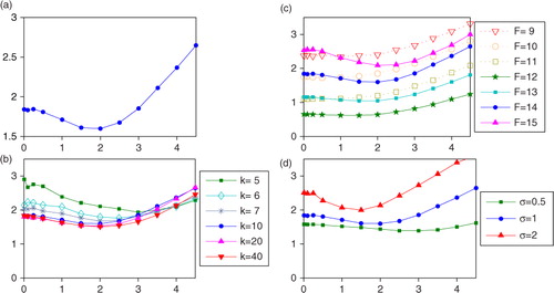
Figure 6a shows the RMSE for various values of η assuming the default parameters. The curve is minimised when η=2.5. Figures 6b–6d show the effect of varying one of the default parameters (k, F, σ), while keeping the other two constant. Thus, the curve in Fig. 6a also appears in Figs. 6b–6d.

Fig. 6 (a–d) The analysis RMSE as a function of η for: (a) our default parameters:an ensemble with k=10 members, model error due to the forcing constant F=14 where the true forcing is F ^t=12, and observation error of 1; (b) various ensemble sizes: k=5, 10, 20 and 40 members; (c) different amounts of model error: F=9, 10, 11, 12, 13, 14 and 15 with F ^t=12; (d) different amounts of observation error: σ=0.5, 1 and 2. In each of (b), (c) and (d), one of the parameters from (a) (k=10, F=14, σ=1) is varied, keeping the other two parameters at their default values; the curve graphed in (a) appears in (b), (c) and (d) as well. We restrict the range of the y-axis in (a) to better show the structure of the curve. (e–h) Comparing the RMSE when η=1 to the minimum RMSE when η is allowed to vary. Subplot (e) shows the percent improvement (of the optimal η versus η=1) in the RMSE with our default parameters, that is, setting η=2.5 gives results with an RMSE, that is, 14% smaller than when η=1. Also shown are the percent improvements versus (f) various ensemble sizes, (g) different forcing constants and (h) different amounts of observation error. Each right hand figure (e), (f), (g) and (h) is derived from the same data as the figure immediately to its left, that is, (a), (b), (c) and (d), respectively.

4.4.2. Varying the ensemble size

Figures 6b and 6f show how varying the ensemble size, k, affects the RMSE and the tuned value of η. We find that FSA improves results more with smaller ensembles than with large ensembles. This may be in part because increasing the ensemble size generally improves the accuracy of the results, so small ensembles have more room to improve their accuracy. It may also reflect the fact that FSA with η>1 accentuates the effect of model nonlinearities on the background ensemble covariance, which could allow greater representation of directions of quickly growing uncertainty that are difficult for a small ensemble to capture. For ensembles with k=10 or more members, the RMSE improvement due to tuning η levels out at around 15%.

4.4.3. Varying the model error

We simulated model error by forecasting the ensemble with a different forcing constant than F ^t=12 used for our truth run. Figures 6c and 6g show how varying the amount of model error (i.e. varying F) can change the effectiveness of tuning η. FSA is more helpful in the presence of model errors that result in to larger amplitude oscillations than the truth, such as when F=13, 14, or 15 and F ^t=12. Averaging the forecast ensemble to produce the background mean tends to reduce the amplitude of these oscillations, and by increasing η we intensify this reduction. We believe this is compensating for some of the model error. We did not find benefits to tuning η in the perfect model scenario or when the forcing constant for the ensemble was smaller than the true forcing constant.

4.4.4. Varying the observation error

Figures 6d and 6e show that effectiveness of FSA and the tuned value of η depend on the size of the observation error σ. As with smaller ensembles, larger observation errors imply larger analysis errors and hence greater room for improvement. The tuned values of η for observation errors of σ=0.5, 1 and 2 are η=4, 2.5 and 1.75, respectively. Thus, more observation error corresponds to a smaller tuned value of η. The ensemble spread in each of these three cases is about 1.8. The ensemble spread roughly determines the size of the difference between the mean of the ensemble forecast and the forecast of the ensemble mean; thus, our finding of an ideal forecast ensemble spread independent of observation error size is consistent with the hypothesis above that ensemble averaging is compensating for some of the model error present.

4.4.5. Approximating the XKF with the ηETKF

Table 2 lists the RMSE from the ηETKF with FSA parameter and 10⁻⁶ and ensembles of size k=40, 60 and 80. We remark that the RMSE associated with the ηETKF approaches the XKF-RMSE from below (increasing the error) as η tends to zero and from above (decreasing the error) as k becomes large.

Table 2. Comparison between the XKF RMSE and the ηETKF RMSEs for and 10⁻⁶ and k=40, 60 and 80 with our default parameters

k=40	k=60	k=80	XKF
η=1	0.88	0.77	0.76
η=1/2	0.95	0.82	0.81
η=1/4	0.97	0.83	0.82
η=1/8	0.97	0.83	0.83
η=10^−6	0.96	0.83	0.83
XKF	0.83

4.4.6. Forecast accuracy

Thus far, we have reported the analysis and background RMSEs for a 6-hour analysis cycle (using Lorenz's conversion of 1 model time unit representing 5 days). We also tested the effect varying η has on the RMSE for forecasts longer than one assimilation cycle. In Fig. 7, we show the 48-hour forecast RMSE, that is, the error in the ensemble mean after the η-adjusted analysis ensemble has been evolved for 48 hours. The absolute improvement from varying η remains similar to the analysis RMSEs shown in Fig. 6, while the η that provides the most improvement is slightly smaller in many cases, including our default parameter case. This could be explained by the greater growth of nonlinear forecast errors with longer lead times, making it appropriate to use less η-inflation.

Fig. 7 RMSE of the mean of a 48-hour η-adjusted ensemble forecast versus the truth. Panels (a), (b), (c) and (d) correspond to the same parameters as in Fig. 6.

5. Summary and conclusions

FSA is a technique that builds upon ensemble data assimilation. After the analysis phase we scale the ensemble perturbations from the mean via multiplication by the factor η, forecasting the adjusted ensemble. Prior to the next analysis, we rescale the perturbations from the background mean by a factor of 1/η before forming the background error covariance matrix.

For linear models, ensemble data assimilation with FSA by any factor η reduces to standard ensemble data assimilation (η=1). For nonlinear models, however, FSA with η≠1 can be beneficial. Further, FSA with a tuned value of η will always perform at least as well as the standard value η=1.

FSA affects the ensemble spread during the forecast phase, so for nonlinear models, an ensemble with a different spread will evolve to a different mean with different perturbation sizes and directions. Like multiplicative covariance inflation, FSA only directly affects the amplitude of the perturbations; it indirectly affects the directions of the perturbations via the nonlinear forecast. In some circumstances, methods such as additive inflation (Houtekamer and Mitchell, 2005; Whitaker et al., 2007), which directly alters the directions of the perturbations, might be more beneficial. Other techniques for inflation such as the relaxation-to-prior-spread (Whitaker and Hamill, 2012) and the relaxation-to-prior-perturbations (Zhang et al., 2004) could also be beneficial, especially with inhomogeneous observation networks. Unlike these techniques, FSA is a type of method that does not assume an optimal or near-optimal error sampling for the forecast phase. We have shown that, while it is important to have the correct statistics during the analysis phase, there can be benefits to a suboptimal error sampling during the forecast phase. As such, FSA could be used in combination with any of the inflation methods described above.

Some authors (e.g. Stroud and Bengtsson, 2007) have found benefits to inflating the observation error covariance, assuming errors in addition to measurement error. In addition to correcting the underestimation of the observation error covariance, they might also be benefiting from the effects of FSA. If the ensembles are identical during the model evolution, then FSA and observation error covariance inflation will produce the same analysis mean and will evolve the same ensemble. This is because both maintain the same the ratio between the background and observation error covariances. The difference is that when inflating the observation error covariance, the size of the assumed errors (P ^b, R ^o and P ^a) is η ² times bigger than those assumed with FSA.

Due to nonlinear effects and model error, an ensemble that appropriately describes the uncertainty at the analysis time will underestimate the uncertainty after it is evolved in time. To compensate for this, many algorithms implement multiplicative covariance inflation on either the background (e.g. Anderson and Anderson, 1999; Whitaker and Hamill, 2002; Miyoshi, 2011) or the analysis (e.g. Houtekamer and Mitchell, 2005; Bonavita et al., 2008; Kleist, 2012). FSA can transition between these two options. Furthermore, FSA can be described as doing both, that is, inflating the analysis error covariance by η ², evolving the ensemble, then inflating the background error covariance by ρ/η ² (which corresponds to deflation if ρ/η ²<1). We prefer to think of the inflation or deflation as happening to the ensemble perturbations from the mean, and we do not consider these perturbations to represent a covariance matrix during the forecast phase.

We demonstrated that the ETKF with FSA (ηETKF) provides a continuum from a reduced-rank XKF (η=0) to the ordinary ETKF (η=1) and beyond. If the ensemble is sufficiently large, we recover the full-rank XKF in the limit η→0. On the other hand, we generally found the lowest analysis errors when η was close to or larger than 1.

We tested FSA with a relatively simple model proposed by Lorenz (2005) to study potential improvements in numerical weather prediction. With our standard parameters, the LETKF with FSA (ηLETKF) improves by 14% upon the standard LETKF. In comparison, a 10 member ensemble with FSA performs better than a 40 member ensemble without FSA. The parameter η tunes to larger than 1 in all scenarios where we saw significant improvements. This corresponds to evolving an ensemble with a larger spread than when η=1. Our standard parameters include model error induced by changing the forcing constant used when evolving the ensemble to a larger value than the true forcing constant. FSA proved even more effective in our tests with a larger forcing constant. However, in perfect model scenarios and when the ensemble forcing constant was smaller than the true forcing, tuning η did not significantly improve the RMSE. Our interpretation of why η>1 improves results when F>12 but not when F≤12 is that larger values of F are associated with higher amplitude oscillations and larger values of η tend to more efficiently reduce these oscillations in the background mean.

In comparison to the RMSE when η=1, tuning η was just as effective in improving the RMSE with ensembles of 40 members as it was with ensembles of 10 members, and was even more effective with ensembles of five members. Lower observation errors increased the tuned value of η in such a way as to suggest that during the forecast phase there is an ideal ensemble spread, that is, relatively independent of the analysis uncertainty. This conclusion is reinforced by the lower value of η desirable for longer term forecasts; the decrease in η can be viewed as compensating for the growth of the ensemble spread over the longer forecast period, keeping the average spread near the ideal. This ideal spread presumably depends on both the model nonlinearity and the model error.

For a more physical model, there may be more significant drawbacks to using values of η significantly larger than 1; in particular, balance (see for example, Daley 1991 Subsection 6.3 or Kalnay 2003 Subsection 5.7) could be an issue. But we argue that at worst, FSA will amplify imbalance already created by the analysis, rather than creating new imbalance. Indeed, if the analysis does not change the ensemble (as would be the case with no observations and ρ=1), then the η-inflation after the analysis simply reverses the η-deflation before the analysis.

In conclusion, FSA with η>1 provided significant improvement compared to η=1 (no adjustment) in some of our experiments with a simple model. FSA was particularly effective for small ensembles, small observation errors and large model errors.

References

- Anderson J. L . Exploring the need for localization in ensemble data assimilation using a hierarchical ensemble filter. Physica. D. 2007; 230: 99–111.
- Anderson J. L , Anderson S. L . A Monte Carlo implementation of the nonlinear filtering problem to produce ensemble assimilations and forecasts. Mon. Wea. Rev. 1999; 127: 2741–2758.
- Bishop C. H , Etherton B. J , Majumdar S. J . Adaptive sampling with the ensemble transform Kalman filter. Part I: theoretical aspects. Mon. Wea. Rev. 2001; 129: 420–436.
- Bishop C. H , Hodyss D . Ensemble covariances adaptively localized with ECO-RAP. Part 1: tests on simple error models. Tellus A. 2009; 61: 84–96.
- Bonavita M , Torrisi L , Marcucci F . The ensemble Kalman filter in an operational regional NWP system: preliminary results with real observations. Q.J.R. Meteorol. Soc. 2008; 134: 1733–1744.
- Buizza R , Houtekamer P. L , Pellerin G , Toth Z , Zhu Y , co-authors . A comparison of the ECMWF, MSC, and NCEP global ensemble prediction systems. Mon. Wea. Rev. 2005; 133: 1076–1097.
- Burgers G , van Leeuwen P. J , Evensen G . Analysis scheme in the ensemble Kalman filter. Mon. Wea. Rev. 1998; 126: 1719–1724.
- Daley R . Atmospheric Data Analysis.
- Evensen G . Using the extended Kalman filter with a multilayer quasi-geostrophic ocean model. J. Geophys. Res. 97: 17905–17924.
- Evensen G . Sequential data assimilation with a nonlinear quasigeostrophic model using Monte Carlo methods to forecast error statistics. J. Geophys. Res. 1994; 99: 10143–10162.
- Evensen G . The ensemble Kalman filter: theoretical formulation and practical implementation. Ocean Dyn. 2003; 53: 343–367.
- Greybush S. J , Kalnay E , Miyoshi T , Ide K , Hunt B. R . Balance and ensemble Kalman filter localization techniques. Mon. Wea. Rev. 2011; 139: 511–522.
- Houtekamer P. L , Mitchell H. L . Data assimilation using an ensemble Kalman filter technique. Mon. Wea. Rev. 1998; 126: 796–811.
- Houtekamer P. L , Mitchell H. L . Ensemble Kalman filtering. Q.J.R. Meteorol. Soc. 2005; 131: 3269–3289.
- Hunt B. R , Kostelich E , Szunyogh I . Efficient data assimilation for spatiotemporal chaos: a local ensemble transform Kalman filter. Physica. D. 2007; 230: 112–126.
- Jazwinski A. H . Stochastic Processes and Filtering Theory.
- Kalman R. E . A new approach to linear filtering and prediction problems. Trans. ASME. Ser. D. J. Basic Eng. 1960; 82: 35–45.
- Kalnay E . Atmospheric Modeling, Data Assimilation and Predictability.
- Kleist D . An Evaluation of Hybrid Variation-Ensemble Data Assimilation for the NCEP GFS. PhD Thesis. University of Maryland, College Park.
- Li H , Kalnay E , Miyoshi T . Simultaneous estimation of covariance inflation and observation errors within an ensemble Kalman filter. Q.J.R. Meteorol. Soc. 2009; 135: 523–533.
- Lorenz E. N . Predictability – a problem partly solved. Proceedings of the Seminar on Predictability. 1996; Reading, Berkshire, UK: ECMWF. 1–18.
- Lorenz E. N . Designing chaotic models. J. Atmos. Sci. 2005; 62: 1574–1587.
- Lorenz E. N , Emanuel K. A . Optimal sites for supplementary weather observations: simulation with a small model. J. Atmos. Sci. 1998; 55: 399–414.
- Miyoshi T . The Gaussian approach to adaptive covariance inflation and its implementation with the local ensemble transform Kalman filter. Mon. Wea. Rev. 2011; 139: 1519–1535.
- Ott E , Hunt B. R , Szunyogh I , Zimin A. V , Kostelich E. J , co-authors . A local ensemble Kalman filter for atmospheric data assimilation. Tellus A. 2004; 56: 415–428.
- Stroud J. R , Bengtsson T . Sequential state and variance estimation within the ensemble Kalman filter. Mon. Wea. Rev. 2007; 135: 3194–3208.
- Wang X , Bishop C. H , Julier S. J . Which is better, an ensemble of positive-negative pairs or a centered spherical simplex ensemble?. Mon. Wea. Rev. 2004; 132: 1590–1605.
- Whitaker J. S , Hamill T. M . Ensemble data assimilation without perturbed observations. Mon. Wea. Rev. 2002; 130: 1913–1924.
- Whitaker J. S , Hamill T. M . Evaluating methods to account for system errors in ensemble data assimilation. Mon. Wea. Rev. 2012; 140: 3078–3089.
- Whitaker J. S , Hamill T. M , Wei X . Ensemble data assimilation with the NCEP global forecast system. Mon. Wea. Rev. 2007; 136: 463–482.
- Zhang F , Snyder C , Sun J . Impacts of initial estimate and observation availability on convective-scale data assimilation with an ensemble Kalman filter. Mon. Wea. Rev. 2004; 132: 1238–1253.