The establishment of Atlantic Water transport as a topographically trapped slope current off Scotland

Abstract

Atlantic Water, with its origin in the western Atlantic, enters the Nordic Seas partly as a barotropic current following the continental slope. This water mass is carried across the Atlantic by the baroclinic North Atlantic Current (NAC). When the NAC meets the continental slope at the east side of the Atlantic, some of the transport is converted to barotropic transport over the slope before continuing northward. Here, we show that this baroclinic to barotropic conversion is in agreement with geostrophic theory. Historical observations show that the transport of the slope current increases significantly from the Rockall Channel (RC) to the Faroe–Shetland Channel (FSC). Geostrophy predicts that with a northward decreasing buoyancy, baroclinic currents from the west will be transferred into northward topographically steered barotropic flow. We use hydrographic data from two sections crossing the continental slope, one located in the RC and another in the FSC, to estimate baroclinic and barotropic transport changes over the slope, within the framework of geostrophic dynamics. Our results indicate that ~1 Sv of the cross-slope baroclinic flow is mainly converted to northward barotropic transport above the 200–500m isobaths, which is consistent with observed transport changes between the RC and the FSC. Similar processes are also likely to occur further south, along the eastern Atlantic margin. This shows that AW within the slope current in the FSC is derived from both the eastern and the western Atlantic, in agreement with earlier studies of AW inflow to the Nordic Seas.

• Atlantic inflow
• North Atlantic Current
• barotropic
• baroclinic

1. Introduction

The inflow of warm and salty Atlantic Water (AW) across the Greenland–Scotland Ridge is a major heat source to the Nordic Seas and Arctic Ocean. Part of the inflow enters the Nordic Seas as a slope current through the Faroe–Shetland Channel (FSC) (Hansen and Østerhus, 2000). The AW in the slope current has two sources: one is water masses with its origin in the western Atlantic carried by branches of the North Atlantic Current (NAC); the other is more saline Eastern North Atlantic Water (ENAW) transported northward by the slope current following the continental margins (McCartney and Mauritzen, 2001; New et al., 2001) (Fig. 1). The transport of AW in the slope current has a dominantly barotropic structure both over the slope off Scotland (Huthnance, 1986) and further north within the Nordic Seas (Fahrbach et al., 2001; Orvik et al., 2001), while the NAC is a mainly baroclinic flow. Thus, the following question arises: How and where does the AW transported by the NAC establish as a barotropic slope current flowing into the Nordic Seas?

Fig. 1 Bottom topography (km) and schematic surface flow (black arrows) in the North-East Atlantic. The major topographic characteristics and flows are marked with their initials. RC—Rockall Channel, WTR—Wyville-Thomson Ridge, FSC—Faroe–Shetland Channel, NAC—North Atlantic Current, SC—Slope Current. The red bars represent two cross-slope hydrographic sections examined in this study: the RC-section (lower) and the FSC-section (upper).

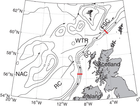
The poleward slope current off Scotland is topographically steered and confined to the upper 500m of the slope (Huthnance, 1986). The volume transport of the flow increases downstream and the largest increase in transport is found where the flow passes the Wyville Thomson Ridge (WTR) (Huthnance, 1986; Huthnance and Gould, 1989). Huthnance and Gould (1989) infer that the increased transport is related to branches of the NAC coming from the west over the WTR and merging with the slope current, which is supported by the observations from six moorings located over the ridge (McCartney and Mauritzen, 2001). However, the mechanism for entraining the AW from the west is still not clear.

The time-mean large-scale current over the slope is essentially a geostrophic flow. Along-slope speeds of the current are generally in the order of 0.1 ms⁻¹, and the continental slope is roughly 20–50km wide (Huthnance and Gould, 1989), thus the Rossby number is in the order of 10⁻¹ or less. Local Ekman transport, generated by a prevailing wind and bottom friction, contributes to the exchange of water properties between the ambient ocean and the shelf (Huthnance, 1995; Holt et al., 2009; Huthnance et al., 2009). Nevertheless, away from the thin Ekman layers, the northward flowing slope current is basically in geostrophic balance.

A classical approach to estimate geostrophic flow from hydrographic data uses thermal wind relation, assuming zero bottom flow or another vertical reference level. This is not very useful at high latitudes, where the flow has large barotropic components. However, the barotropic flow component follows the isobaths and the bottom density field can determine its along-slope evolution. Note that Fofonoff (1962) is the first to show that geostrophic flow can be split into a depth-independent barotropic component and a depth-dependent baroclinic component, and he also mentions that the barotropic component is proportional to the bottom density anomaly. More recently, this has been used to diagnose geostrophic flow from observed bottom densities within the Nordic Seas and Arctic Ocean. Schlichtholz (2002, 2007) uses this method with success to characterise the circulation in the East Greenland Current. Walin et al. (2004) use it to develop a simplified model of the Nordic Seas describing important features of the boundary current over the continental slope. Nilsson et al. (2005) find that when used within closed topographic contours, the density dependent bottom flow can be described using a simple geostrophic model. This model is later used to diagnose the circulation in the Nordic Seas and Arctic Ocean (Aaboe and Nøst, 2008), and the diagnosed circulations agree well with observations (Aaboe et al., 2009). Note that this method does not say anything about the driving forces of the flow, but only diagnoses the geostrophic flow. As long as the Rossby number of the flow is small, the diagnosis will describe the characteristic features of the flow, regardless of the mechanisms setting up the flow. Similarly, when we use the thermal wind relation to estimate and describe the flow through a section, it is only a description of the geostrophic flow, which is valid when the Rossby number is small.

In this study, we diagnose the slope current using hydrographic data within the framework of geostrophic theory. The slope current loses heat to its surroundings by eddy shedding and heat loss to the atmosphere, leading to a downstream decreasing buoyancy (McCartney and Mauritzen, 2001). Our hypothesis is that the along-slope density gradients provide an explanation for how the AW, brought across the Atlantic by the NAC, is established as a barotropic slope current flowing into the Nordic Seas. The rest of this paper is organised as follows. Section 2 briefly reviews the theory, and Section 3 presents the data used in the analysis. Estimations of baroclinic to barotropic transport conversion are given in Section 4, followed by a discussion in Section 5.

2. Geostrophic flow over a sloping boundary

For a steady-state large-scale circulation away from boundary layers, the momentum equation can be approximated in geostrophic and hydrostatic balances,1 2

Here, v is the horizontal velocity component, f is the Coriolis parameter, k is the vertical unit vector, ρ₀ is the reference density, p is the pressure, ∇ is the horizontal gradient operator, g is the acceleration of gravity, ρ is the density and z is the vertical coordinate. Integrating eq. (2) from the bottom (z=−H) to a depth z gives the pressure relative to bottom pressure, p _b . Then, using this in the geostrophic relation [eq. (1)] gives the following expression for geostrophic velocity,3

which can be expressed as follows using Leibnitz's rule4

where ρ _b is the bottom density. In eq. (4), the first two terms on the right are independent of depth while the last term, the integrated thermal wind relative to bottom, is depth-dependent and equals zero at z=−H. We define the depth-independent part of the velocity as barotropic and the depth-dependent part as baroclinic, following Fofonoff (1962).

In a geostrophic flow on an f-plane, the velocity is non-divergent. This is satisfied by the term including p _b and by the second term on the right of eq. (3), which is split into a barotropic and baroclinic term in eq. (4). Therefore, from eq. (4) we see that a divergence (convergence) in the barotropic velocity is balanced by a convergence (divergence) in the baroclinic velocity. The barotropic and baroclinic flow is intimately connected.

The along-slope bottom velocities in our region of interest are in the order of 0.1 ms⁻¹ (Huthnance, 1986; McCartney and Mauritzen, 2001). Nøst and Isachsen (2003) show that for velocities of this order of magnitude in combination with topographic gradients larger than 10⁻³, p _b can be approximated as a function of depth. Following Nøst and Isachsen (2003), we see that the velocity given by p _b in eqs. (3) and (4) will be directed along the slope and its associated along-slope transport will be constant and non-divergent. As we are interested in the interaction between baroclinic and barotropic flow, we will focus on the flow represented by the last two terms on the RHS of eq. (4). Integrating these two terms over the water column defines the transport V,5

V is not a measure of the total along-slope transport, which also requires the terms involving p _b . However, it contains all information about along-slope barotropic transport changes and the associated interaction between barotropic and baroclinic transports due to along-slope density variation.

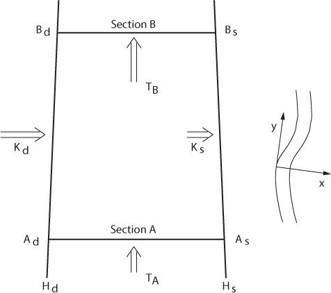
We will investigate the different components of V to explore the interaction between barotropic and baroclinic transports within the box area illustrated by Fig. 2. The area is limited by two isobaths, H _d (the deeper one) and H _s (the shallower one) and two cross-slope sections, A and B. V consists of cross- and along-slope baroclinic transports and along-slope barotropic transport. The cross-slope baroclinic component integrated between sections A and B on a given isobath is:6

Fig. 2 Illustration of a box area over a slope. x and y are the cross-slope and along-slope coordinates respectively.

where y is the along-slope coordinate and ρ _A(B) is the density profile at the section A(B) above a given isobath. The along-slope baroclinic component integrated between the two isobaths H _d and H _s is:7

which can be further expressed as:8

Here, x is the cross-slope coordinate and ρ_{H d (H s )} is the density profile at the isobath H _d (H _s ) at a given section. The along-slope barotropic component of V integrated between the two isobaths H _d and H _s, is:9

Using the f-plane assumption leads to ∇·V=0, which again leads to:10

where is the along-slope transport change and the cross-slope baroclinic transport change within the box area. A divergence (convergence) of along-slope barotropic transport will lead to a convergence (divergence) of baroclinic transports. Since the bottom density determines the along-slope barotropic transport, there is always interaction between barotropic and baroclinic flow if it exists along-slope bottom density gradients. Note that the geostrophic cross-slope transport ΔK should not be seen as an estimate of total cross-slope transport which also involves other ageostrophic processes.

As we already addressed at the beginning of this section, all of the estimates are based on the geostrophic approximation, the validity of which can be estimated from the bottom density as follows. The geostrophic approximation is justified if the Rossby number U/fL is sufficiently small. Here U is the velocity change and L is the distance over which velocity changes. In the box area (Fig. 2), U can be expressed in terms of ΔK or ΔT_ρb . If we assume that changes in cross-slope baroclinic flow (ΔK) are mainly converted to along-slope barotropic flow (ΔT_ρb ) (results in Section 4 show that this is a good approximation), we can write:11

Using this velocity scale, we obtain the following expression for the Rossby number R,12

This equation estimates the Rossby number R from the along-slope bottom density variation δρ _b , the cross-slope length scale L, and the water depth, H. We will use this to check the validity of the geostrophic approximation, which our results depend on.

3. Data

As illustrated in the theory section, bottom density is a key variable both for examining the along-slope barotropic transport and for checking the validity of the geostrophic approximation. Distributions of bottom densities on the 200–700m isobaths with 100m depth interval over the slope off Scotland are obtained as follows. Coordinates of each isobath are constructed from the ETOPO2 data from the National Geophysical Data Center, by using the contour function of Matlab. Historical bottom hydrographic data from 1985–2005 are achieved from the International Council for the Exploration of the Sea (ICES) and the British Oceanographic Data Centre (BODC) databases. Note that the data points are not always located on the exact isobaths of their water depths due to measurement uncertainties or resolution/error of the topographic data set. The hydrographic data are first sorted according to water-depth into six depth bins, one for each isobath, i.e. 150–250m for the 200m isobath, 250–350m for the 300m isobath and so on. At each depth bin, only data points with distance to the corresponding isobath<10km are used to estimate bottom density. For each observation, we find the nearest point on the isobath. The bottom density on each point of the isobath is set to the mean of all observed densities having this point as their nearest point. Points on the isobath that are not the nearest point to any observations are not given a density value. Resulting bottom densities are shown in Fig. 3.

Fig. 3 Bottom densities against latitudes along each isobath. Black lines indicate where the WTR meets the slope, and thick grey lines indicate the RC-section (left) and the FSC-section (right).

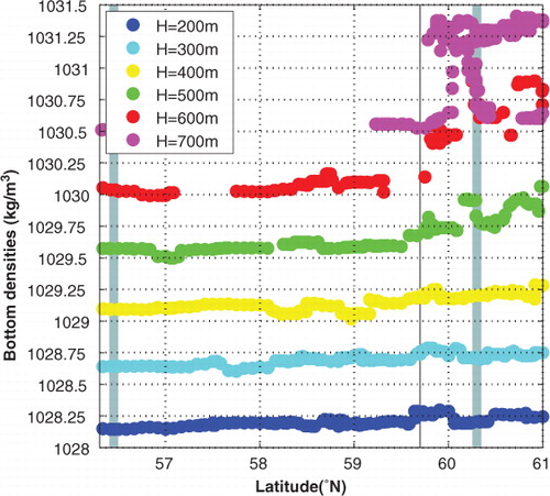
Despite the non-synopticity of the data, densities on all isobaths show a clear northward increasing trend. A closer look at Fig. 3 shows that bottom densities on the 200 and 300m isobaths increase slightly from south to north (~0.1kg/m³). Bottom densities along the 400 and 500m isobaths are near constant south of the WTR and increase rapidly when passing the ridge and northward, both with an increase >0.2kg/m³. Bottom densities on both the 600 and 700m contours are also near constant south of the WTR. While passing the ridge and northward, bottom densities on the 600m isobath jump from ~1030 to near 1031kg/m³. The reason for this is that north of the WTR, the 600m isobath is occupied by dense overflow water and not AW. The bottom densities on the 700m isobath look more complicated because this isobath detours around the WTR while we use latitude as the x-coordinate, and water masses on this isobath switch between AW and overflow water.

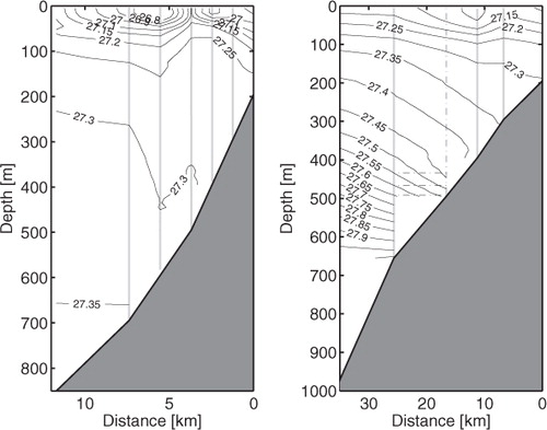
To quantitatively examine the interaction between baroclinic and barotropic flow, two hydrographic cross-slope sections have been selected and CTD casts from these two sections are obtained from the ICES and BODC databases. As shown in Fig. 1, one section is located right across the Scottish continental slope at the RC (56.45°N, RC-section hereafter). This section has been surveyed regularly during the years 1995–1996 (Souza et al., 2001). The other section is the Fair Isle-Munken in the FSC (around 60.3°N, FSC-section hereafter), which has been monitored routinely since 1903 (Hansen and Østerhus, 2000). Here, we only use observations taken at the Shetland side with the same period as the RC-section, from 1995 to 1996. Figure 4 shows the mean potential densities along the two sections.

Fig. 4 Mean potential densities (kg/m³) from the CTD casts along the RC-section (left) and the FSC-section (right). In the left panel, grey vertical solid lines indicate the positions of the 700, 600, 500, 400 and 300m isobaths. In the right panel, grey vertical solid lines indicate the positions of the 660, 400 and 300m isobaths, while the dashed grey line indicates the 500m isobath above which there are no direct observations. Horizontal black dashed lines indicate constant densities extending from the 660m isobath to the 500m isobath below 400m.

To estimate the different transport components [eq. (6), (8) and (9)], vertical density profiles are constructed above isobaths at the two sections as follows. Along the RC-section, down-to-bottom CTD profiles exist between 100 and >1000 m depth. Mean vertical density profiles above each isobath (200, 300, 400, 500, 600, 700 and 850m) are constructed by averaging T and S observations onto a regular vertical grid with 10 m spacing. During the averaging, only profiles with depths within 30m to the isobath depth are used. In each bin, the uncertainty of the mean salinity (temperature) e _S(T) is given by (Taylor, 1982):13

where σ _S(T) is the standard deviation for the mean salinity (temperature) and N is the number of observations within each bin.

Along the FSC-section, profiles only exist above fixed bottom depths (200, 325, 400, 660 and 1000m). The profiles above the 200, 300 and 400m are constructed similarly as for the RC-section, but for the 500m isobaths, we use two alternative methods. When finding the representative profile for the 500m isobath, we first linearly interpolate T and S profiles for the upper 400m from the profiles for the 400 and 660m isobaths. The uncertainties of the interpolated salinities (temperatures) e _500S(T) are given by:14

where e _400S(T) and e _660S(T) are the uncertainties of mean salinities (temperatures) for the 400 and 660m isobaths, respectively. Note that eq. (14) represents the upper limit of uncertainties for linear interpolation, according to Taylor (1982). This is applied throughout the paper when estimating uncertainties for linear interpolation. From 400m to bottom, the S and T values are obtained by two kinds of extrapolation, one extends the mean values for the 660m isobath to the 500m isobath assuming horizontal isopycnals (method E1), and the other linearly extrapolates from values of the 1000 and the 600m isobaths assuming constant isopycnal slopes (method E2). This time, the uncertainties of the extrapolated salinities (temperatures) are taken the same values as those for the 660m isobath within 400–500m depth. This is a rough way of estimating uncertainties for extrapolation, but it should not affect our results significantly since only values on one fifth of the profile depth are obtained by extrapolation.

Density profiles for each isobath are calculated from mean salinities and temperatures (UNESCO, 1983); while the equation of state is approximated as a linear function of temperature and salinity when estimating uncertainties, as follows.15

where β _S =7.6×10⁻⁴ ppt ⁻¹, β _T =2×10⁻⁴ K ⁻¹ and β _p =4.1×10⁻¹⁰ Pa ⁻¹. T ₀, S ₀, p ₀ are constants for temperature, salinity and pressure respectively. These constants and the pressure p are ignored when estimating uncertainties. Thus, the propagation of uncertainties for linear combinations is used for estimating uncertainties of densities:16

The deepest part of the along-slope baroclinic transport [second term of eq. (8)] cannot be estimated from vertical density profiles above the two isobaths, because this area is deeper than the shallower isobath. To find the horizontal density gradient, we first linearly interpolate the bottom density onto the seabed (linearly interpolated between H _d and H _s ) between the two isobaths. Densities from the vertical profile above the deeper isobath are then used together with bottom densities at the same depth between the two isobaths to estimate the horizontal density gradient as a function of z. This is then integrated to estimate the second term of eq. (8).

4. Conversion from baroclinic to barotropic flow

Before we estimate geostrophic transport changes, we check the validity of the geostrophic approximation by examining Rossby numbers along the isobaths according to eq. (12). Here, we use the values f=1.2×10⁻⁴ s ⁻¹, ρ₀=1.029×10³kg/m³ and g=9.8 m/s². The variation of the Coriolis parameter f from the RC-section to the FSC-section is within 3% of a constant value, so that f-plane is a reasonable assumption. As we mentioned in Section 3, bottom density variation δρ_b is at the order of 10⁻¹ or less along the 200–500m isobaths, over a length scale of hundreds of kilometres. In contrast, δρ_b is at the order of 1kg/m³ along the 600–700m isobaths over a short distance. We choose L=10km because this is a characteristic cross-slope length scale for the slope current. Rossby numbers are generally small along the 200–500m isobaths, with a magnitude of 10⁻¹ or less, indicating that the geostrophic balance is a reasonable approximation for the slope current above these depths in the cross-slope direction. However, Rossby numbers along the 600 and 700m isobaths are near or larger than unity around the area of the WTR, suggesting that geostrophic balance breaks down over the slope deeper than 500m. Therefore, we only estimate the transport changes between the 200 and 500m isobaths.

In general, our estimates of the Rossby numbers are in good agreement with studies of the flow regime in this region. In the FSC, depths <500m are mainly occupied by southward flowing overflow water (Hansen and Østerhus, 2000). The overflow exits the FSC and descends into the Atlantic either through Faroe Bank Channel or over the WTR (Mauritzen et al., 2005). The overflow in the Faroe Bank Channel is hydraulically controlled from analysis of observations (Girton et al., 2006 ; Hansen and Østerhus, 2007), and the overflow cascading over the WTR could also be subject to hydraulic control (Sherwin and Turrell, 2005). This indicates that our simple geostrophic approach cannot be applied to the isobaths (600 and 700m) between the two sections, due to the fact that the flow at these depths has been exposed to ageostrophic processes.

The baroclinic transports K, T _r and the barotropic transport T_ρb are estimated on each isobath from the density profiles at the two sections according to eqs. (6), (8) and (9). Before the integration in eq. (9), ρ_b is linearly interpolated with respect to H. Corresponding transport changes ΔK, ΔT _r and ΔT_ρb , within the volume separated by neighbouring isobaths and the two cross-slope sections, are listed in Table 1. The uncertainties listed in parenthesis are obtained from methods of propagation of uncertainties described earlier in Section 3. There are, of course, other sources of uncertainties, one being the interpolation of bottom densities onto the 500m isobath at the FSC section (E1 and E2, see Table 1), which clearly gives different values of the transport changes. However, the uncertainties in parenthesis give an estimate of how variability in the observations contributes to uncertainties.

Table 1. Estimated cross-slope transport change (ΔK) and along-slope transport change (ΔT_ρb , ΔT _r) from the RC-section to the FSC-section within two neighbouring isobaths. Values in parenthesis are uncertainties

500–400 m
Transport change	E1	E2	400–300m	300–200m
ΔK (Sv)	−1.0 (±0.1)	−0.61 (±0.04)	−0.20 (±0.06)	−0.07 (±0.03)
ΔTρb (Sv)	0.7 (±0.03)	0.51 (±0.04)	0.18 (±0.06)	0.07 (±0.03)
ΔT r (Sv)	0.25 (±0.01)	0.12 (±0.01)	0.01 (±0.01)	0.0005 (±0.005)

The sum of ΔK, ΔT _r and ΔT_ρb equals zero within the uncertainties, which agrees well with the prediction from eq. (10). The estimates of T _r account only for a small fraction of ΔT_ρb or ΔK, which highlights that the conversion is mainly from cross-slope baroclinic flow to along-slope barotropic flow [which also justifies the approximation used to derive eq. (12)]. Between the 500 and 400m isobaths, estimates from both methods (E1 and E2) indicate that most of the change in cross-slope baroclinic flow is converted into along-slope barotropic flow. We do not know which of the two methods is better. However, by using a mean of the two estimates we conclude that the cross-slope baroclinic transport decreases by ~0.8 Sv within the 500–400m depth while ~0.6 Sv of it has turned into along-slope barotropic transport and ~0.2 Sv into along-slope baroclinic transport. Similarly, the barotropic transport increase between the 400 and 300m isobaths (~0.18 Sv) is mainly caused by a cross-slope baroclinic transport decrease (~0.20 Sv). Further shoreward between the 300 and 200m isobaths, the same conclusion can be reached; cross-slope baroclinic transport is mainly converted into along-slope barotropic transport. In total, the cross-slope baroclinic transport decreases by ~1 Sv within the 200–500m depth, of which ~0.85 Sv is converted to the along-slope barotropic transport.

5. Summary and discussion

In this study, we examined the conversion from baroclinic to barotropic flow in the slope current over the continental slope off Scotland using hydrographic data within the framework of geostrophic theory. Our estimates show that ~85% of the cross-slope baroclinic flow is transformed into along-slope barotropic flow from 56.5°N in the RC to 60.3°N in the FSC between the 200 and 500m isobaths. This causes the northward barotropic flow to increase by ~0.85 Sv between these two sections.

How do our estimates compare to direct observations of volume transport of the slope current? Huthnance (1986) reports transports of the slope current to be 1.5 Sv inshore of the 2000 m isobath at 58°N and 1.0 Sv inshore of the 500m isobath at 59°N. Since the flow is reported to be essentially barotropic (Huthnance, 1986), this indicates that the barotropic transport at the RC section is in the order of 1 Sv. Sherwin et al. (2008) report that the time mean transport of AW (in the period from 1995 to 2005) above 500m in the FSC is 3.5 Sv, where the barotropic component of the transport is 2.1 Sv. The estimated barotropic flow is located over the upper slope, which makes it directly comparable to our estimates between the 500 and 200m isobaths. From this information, the barotropic transport increase from the RC to the FSC should then be 1.1 Sv. Of course, this number is subject to large uncertainties, and we believe it is fair to conclude that direct measurements indicate a barotropic transport increase between the RC and the FSC of ~1 Sv, which is in good agreement with our estimate of 0.85 Sv.

Our study provides an understanding of how the AW carried by the baroclinic NAC establishes itself as a barotropic flow over the slope while crossing the WTR. The geostrophic flow over the continental slope experiences buoyancy loss leading to a conversion from baroclinic to barotropic flow trapped over the slope. As shown in Fig. 3, the bottom densities increase significantly where the WTR meets the slope and further northward, indicating that most of the baroclinic flow of AW is converted to barotropic flow around this area. Therefore, our results qualitatively support the (Huthnance and Gould, 1989)'s inference that the large transport increase of the slope current is related to the AW coming from west over the WTR.

The northward transport of the slope current is also increasing further south, from the Bay of Biscay. According to Pingree and Le-Cann (1989), the volume transport of the slope current increases from ~0.6 Sv between 1000m depth and the shelf break at ~47.5°N to ~1 Sv at the RC. In this region, the amount of available hydrographic data is much less, making a study of geostrophic conversion from baroclinic to barotropic flow difficult. However, a look at the limited available data indicates a northward density increase also in this region (not shown), suggesting that AW from the west may be entrained into the slope current also here. According to this, the AW flowing into the Nordic Seas within the slope current is derived from water masses near the continental margin at the Bay of Biscay, in addition to the AW from the NAC entrained into the slope current on its way northward. This is in agreement with New et al. (2001), who argue that the AW flowing into the Nordic Seas is a mixture of westerly derived AW carried by the NAC and ENAW carried northward by the slope current from the Bay of Biscay.

Our study may be criticised for applying a simple geostrophic approach to describe the slope current at the shelf break region where ocean dynamics is complicated. Besides the topographically steered slope current, ageostrophic processes, namely wind stress, bottom friction eddies and tides, interact and play a key role in setting up the slope current and maintaining ocean-shelf exchange (Huthnance, 1995). Nevertheless, we emphasise that we do not study the dynamic balance setting up the slope current, instead we simply describe the slope current based on characteristics of geostrophic flow over a sloping boundary. When the slope current is mainly geostrophic, it will behave as described by the geostrophic equations independent of the dynamical balances setting up the flow. Note that these ageostrophic processes are not totally ignored in our study; they are crucial in setting up the along-slope density gradients and thus affect the along-slope transport of the slope current.

The geostrophic approach that we use in this work is a powerful tool for diagnosing geostrophic flow over topography. Geostrophy can be used to diagnose topographically steered barotropic flow, which makes it especially useful for high-latitude oceanography. In fact, geostrophy provides an understanding of why high latitude circulation is often topographically steered with a strong barotropic component: High latitude flow mainly loses buoyancy to its surroundings, leading to a conversion from baroclinic flow to topographically trapped barotropic flow.

6. Acknowledgments

This research was supported by the Norwegian Research Council through the project POCAHONTAS. The authors are grateful for discussions with colleagues, Signe Aaboe and Tore Hattermann. Reviewer comments helped to improve the presentation greatly.

References

- Aaboe S , Nøst O. A . A diagnostic model of the Nordic Seas and Arctic Ocean circulation: quantifying the effects of a variable bottom density along a sloping topography. J. Phys. Oceanogr. 2008; 38: 2685–2703.
- Aaboe S , Nøst O. A , Hansen E . Along-slope variability of barotropic transport in the Nordic Seas: simplified dynamics tested against observations. J. Geophys. Res. 2009; 114: C03009.
- Fahrbach E , Meincke J , Østerhus S , Rohardt G , Schauer U , co-authors . Direct measurements of volume transports through Fram Strait. Pol. Res. 2001; 20(2): 217–224.
- Fofonoff N. P , Hill M. N , Goldberg E. D , O'D Iselin C , Munk W. H . Dynamics of ocean current. The Sea. 1962; 323–395.
- Girton J. B , Pratt L. J , Sutherland D. A , Price J. F . Is the Faroe Bank Channel overflow hydraulically controlled?. J. Phys. Oceanogr. 2006; 36: 2340–2349.
- Hansen B , Østerhus S . North Atlantic – Nordic Seas exchanges. Progr. Oceanogr. 2000; 45: 109–208.
- Hansen B , Østerhus S . Faroe Bank Channel overflow 1995–2005. Prog. Oceanogr. 2007; 75: 817–856.
- Holt J , Wakelin S , Huthnance J . Down-welling circulation of the northwest European continental shelf: a driving mechanism for the continental shelf carbon pump. Geo-phys. Res. Lett. 2009; 36 L14, 602.
- Huthnance J . The Rockall slope current and shelf-edge processes. Proc. Roy. Soc. Edinb. 1986; 88B: 83–101.
- Huthnance J , Gould W , Neshyba S. J , Mooers C. N. K , Smith R. L , Barber R. T . On the northeast Atlantic slope current. Polarward Flows along Eastern Ocean Boundaries. 1989; 76–81. Springer-Verlag, New York.
- Huthnance J , Holt J , Wakelin S. L . Deep ocean exchange with west-European shelf seas. Ocean Sci. 2009; 5: 621–634.
- Huthnance J. M . Circulation, exchange and water masses at the ocean margin: the role of physical processes at the shelf edge. Progr. Oceanogr. 1995; 35: 353–431.
- Mauritzen C , Price J , Sanford T , Torres D . Circulation and mixing in the Faroese channels. Deep-Sea Res. I. 2005; 52: 883–913.
- McCartney M. S , Mauritzen C . On the origin of the warm inflow to the Nordic Seas. Progr. Oceanogr. 2001; 51: 125–214.
- New A , Barnard S , Herrmann P , Molines J . On the origin and pathway of the saline inflow to the Nordic Seas: insights from models. Progr. Oceanogr. 2001; 48: 255–287.
- Nilsson J , Walin G , Broström G . Thermohaline circulation induced by bottom friction in sloping-boundary basins. J. Mar. Res. 2005; 63: 705–728.
- Nøst O. A , Isachsen P. E . The large-scale time-mean ocean circulation in the Nordic Seas and the Arctic Ocean estimated from simplified dynamics. J. Mar. Res. 2003; 61: 175–210.
- Orvik K. A , Skagseth Ø , Mork M . Atlantic inflow to the Nordic Seas: current structure and volume fluxes from moored current meters. VM-ADCP and SeaSoar-CTD observations, 1995–1999. Deep Sea Res. 2001; 48: 937–957.
- Pingree R , Le-Cann B . Celtic and Armorican slope and shelf residual currents. Progr. Oceanogr. 1989; 23: 303–338.
- Schlichtholz P . On a modified arrested topographic wave in Fram Strait. J. Geophys. Res. 2002; 107(C11): 3189.
- Schlichtholz P . Density-dependent variations of the along isobath flow in the East Greenland Current from Fram Strait to Danmark Strait. J. Geophys. Res. 2007; 112: C12022.
- Sherwin T , Hughes S , Turrell W , Hansen B , Østerhus S . Wind-driven monthly variations in transport and the flow field in the Faroe–Shetland Channel. Pol. Res. 2008; 27: 7–22.
- Sherwin T. J , Turrell W. R . Mixing and advection of a cold water cascade over the Wyville Thomson Ridge. Deep-Sea Res. I. 2005; 52: 1392–1413.
- Souza A , Simpson J , Harikrishnan M , Malarkey J . Flow structure and seasonality in the Hebridean slope current. Oceanologica Acta-Supplement. 2001; 24: S63–S76.
- Taylor J. R . An Introduction to Error Analysis: The Study of Uncertainties in Physical Measurements. 1982. University Science Books, Mill Valley, California.
- Walin G , Broström G , Nilsson J , Dahl O . Baroclinic boundary currents with downstream decreasing buoyancy; a study of an idealised Nordic Sea system. J. Mar. Res. 2004; 62: 517–543.