Ensemble-based observation impact estimates using the NCEP GFS

Abstract

The impacts of the assimilated observations on the 24-hour forecasts are estimated with the ensemble-based method proposed by Kalnay et al. using an ensemble Kalman filter (EnKF). This method estimates the relative impact of observations in data assimilation similar to the adjoint-based method proposed by Langland and Baker but without using the adjoint model. It is implemented on the National Centers for Environmental Prediction Global Forecasting System EnKF that has been used as part of operational global data assimilation system at NCEP since May 2012. The result quantifies the overall positive impacts of the assimilated observations and the relative importance of the satellite radiance observations compared to other types of observations, especially for the moisture fields. A simple moving localisation based on the average wind, although not optimal, seems to work well. The method is also used to identify the cause of local forecast failure cases in the 24-hour forecasts. Data-denial experiments of the observations identified as producing a negative impact are performed, and forecast errors are reduced as estimated, thus validating the impact estimation.

• data assimilation
• observation impact
• ensemble Kalman filter
• skill dropout
• ensemble sensitivity

1. Introduction

The quality of the initial conditions is very important for the accuracy of the numerical weather prediction (NWP). The assimilation of observations should improve the initial conditions if they are assimilated properly. Therefore, estimating the observation impacts within the NWP system is an important step towards improving the performance of the operational NWP. The information on observation impacts is essential for the design of future observing systems producing information on the usefulness of specific components of the observing system that can be combined with the costs of the observing system to allow a more efficient allocation of resources. It also provides important guidelines for the development of the data assimilation systems, indicating which components of the observing system are being used most completely and can indicate which observation types need improvement in their use [e.g. quality control (QC), improved forward models, observation errors, etc.].

There have been substantial efforts to estimate the impact of the assimilated observations by carrying out data-denial experiments or the Observing System Experiments (OSEs, e.g. Bouttier and Kelly, 2001; Zapotocny et al., 2007, 2008). OSEs provide the nonlinear impacts on the accuracy of the forecasts with and without a certain set of observations. However, carrying out OSEs with various observation datasets is computationally very expensive. As an alternative, Langland and Baker (2004) proposed a pioneering method to estimate the observation impacts on the forecasts without performing OSEs by using an adjoint sensitivity analysis. Their forecast sensitivity to observations approach can be performed at a relatively low computational cost and provides the impact of each assimilated observation in a linear sense. It has been applied to several operational data assimilation systems and has been proven to be an effective method of estimating the observation impacts on the short-range forecasts and the performance of the data assimilation system (e.g. Zhu and Gelaro, 2008; Cardinali, 2009). However, it requires the adjoint operators of the forecast model and of the data assimilation system. Hakim and Torn (2008) and Ancell and Hakim (2007) proposed an ensemble sensitivity method assuming a linear relationship between ensemble forecast (or error of ensemble forecast) and analysis ensemble to generate forecast sensitivity to the analysis without an adjoint model. This method can also be extended to derive observation impacts with a relatively small number of observations. Liu and Kalnay (2008) and Li et al. (2010) proposed another method using the ensemble Kalman filter (EnKF) to estimate observation impacts directly without the adjoint model. The ensemble-based approach is convenient for estimating the observation impacts in the ensemble-based data assimilation system since it uses the ensemble perturbations instead of the adjoint model to derive sensitivity of forecast errors to the analysis. Kunii et al. (2012) successfully applied the Liu and Kalnay (2008) method to estimate the impact of real observations with the Weather Research and Forecasting model using the local ensemble transform Kalman filter (LETKF, Hunt et al., 2007) and estimated the impact of various observations on the Typhoon Sinlaku forecast. Kalnay et al. (2012) proposed an improved formulation of the Liu and Kalnay (2008) algorithm. It is simpler, makes fewer approximations and can be applied to other deterministic EnKFs, and not just to the LETKF.

In this study, observation impact estimates within the EnKF are investigated. The formulation of Kalnay et al. (2012) is applied to the National Centers for Environmental Prediction (NCEP) Global Forecasting System EnKF (GFS/EnKF, Whitaker et al., 2008) with the observations assimilated in the NCEP operational global data assimilation system. The results provide the relative impacts of each observing system in the operational NWP context. We show that the formulation can also be used as an effective tool to investigate the origin of local forecast error that sometimes substantially degrades the operational forecasts. Section 2 introduces the formulation of the ensemble-based approach used in this study. Following Section 3 with the experimental settings, Section 4 presents the overall impact estimation results, and Section 5 focuses on the estimation of the origin of local forecast failures. Finally, Section 6 provides a summary and discussion.

2. Ensemble-based formulation

We would like to estimate the forecast error reduction due to the assimilation of each observation. The forecasts from the analysis () and from the first guess () are verified against the analysis or any other values close to the truth () at forecast time t. We define the forecast errors as1

The overbars represent the ensemble mean and can be disregarded for the deterministic analysis and forecast. Following Langland and Baker (2004), forecast error reduction is defined as2

where C is the norm operator, defining the measure of the forecast error. The forecast error difference can be described as3

where and are the analysis and the first guess at time 0. M and K represent the tangent linear forecast model and Kalman gain matrix, respectively. Here, , is the vector of innovations, where y _o is the observation vector and H the nonlinear observation operator. The forecast time t is assumed to be short, so that the tangent linear model assumption is appropriate. From eqs. (2) and (3), the forecast error reduction from the assimilation of observations is expressed as4

This equation is used for the observation impact estimates based on the adjoint sensitivity. In the EnKF, the Kalman gain is given by5

where K, , A and R are the ensemble size, the matrix of analysis perturbations, the analysis error covariance and the observation error covariance, respectively. As a result, eq. (4) can also be written as6

This equation is used for this study to estimate observation impacts. It is simpler and computationally more efficient than the original formulation of Liu and Kalnay (2008) and Li et al. (2010) and can also be easily applied to deterministic EnKFs other than the LETKF (Kalnay et al., 2012).

As the EnKF requires covariance localisation when the number of degrees of freedom is much larger than the number of the ensemble members, the ensemble-based observation impact estimates also require localisation in practical applications. Following Kalnay et al. (2012), we achieve this by computing the impact of lth observation on forecast at jth grid point as7

where ρ _j is the localisation function at grid point j for the l ^th observation. Note that the localisation function in eq. (7) may be different from the one used in the EnKF analysis especially when the impact of the observations on the forecast propagates away from the initial location.

Using the same approximation applied in eq. (6), the impact of any subset of observations can also be estimated as8

where superscript ‘part’ means a partial set of observations. The impact can be computed with lower computational cost than in data-denial experiments provided that the ensemble forecast from the EnKF analysis is already available since no additional forecasts need to be produced.

Ancell and Hakim (2007) proposed to use an ensemble sensitivity method to estimate the impact of additional observations to the forecast [eq. (28) in their paper]. Under certain conditions, this method is closely related to eq. (8) (see Appendix).

3. Experimental settings

Equation (7) is applied to the NCEP GFS/EnKF analysis and forecast ensembles. The horizontal resolution of the GFS in this experiment is T254 (about 55 km) and it has 64 sigma-p hybrid vertical layers up to 0.3 hPa. The serial Ensemble Square Root version of EnKF (EnSRF, Whitaker and Hamill, 2002) is used to produce an ensemble of analyses. The EnKF employs 80 members and assimilates observations every 6 hours. The forecast errors with both dry and moist total energy norms (Ehrendorfer et al., 1999) in the global domain are used for the impact estimation and the verifications are made against its own analysis.9

Here u′, v′, T′, and q′ are the forecast errors of zonal wind, meridional wind, temperature, surface pressure and specific humidity, respectively. C _p, R _d and L are the specific heat at constant pressure, gas constant of dry air and latent heat of condensation per unit mass, respectively. T _r and P _r are a reference temperature and pressure, respectively (we used 280 K and 10⁵ Pa). w _q is 1 for moist total energy and 0 for dry total energy. Equation (9) is used as forecast error norm C in eq. (7). The use of ensembles allows us to estimate the impact in both dry and moist total energy at the same time without additional computational cost since eq. (7) can be explicitly decomposed into each forecast variable. The evaluation forecast time is chosen to be 24 hours.

Covariance localisation is applied in the EnKF analysis to reduce the sampling noise from the member-limited ensemble-based covariance estimate. The localisation reduces the correlation between observation priors and first guess ensembles from the raw ensemble correlation. The reducing factor is a function of the distance between observations and analysis grid points. The fifth-order polynomial of Gaspari and Cohn (1999) approximating a Gaussian function (eq. (4.10) in their paper) is used as the covariance localisation function with a cutoff length (where localisation function becomes 0) at 2.0 scale heights for the vertical and 2000 km for the horizontal (corresponding to an e-folding scale of 0.8 scale heights and 800 km, respectively).

The localisation scale for the observation impact estimate is chosen to be the same as for the EnKF analysis update. However, since observation impacts evolve through the forecast model evolution, the localisation function should also evolve. We tested both a fixed localisation function as in the EnKF analysis and a moving localisation function with the centre position moving proportionally to the average of analysis and forecast horizontal wind at each vertical level in order to partially account for the effect of the propagation of the observational impact by the mean flow. The coefficient that multiplies the average horizontal wind is tuned so that the global forecast error reduction estimate is approximately maximum (a value of 0.75 is used). Multiplicative inflation (Anderson, 2001) proportional to the spread reduction by analysis update is applied so that the amount of spread reduction becomes 15% of the original reduction. Additive inflation using 0.32 times randomly selected 24- and 48-hour forecast lagged differences is also applied. These are the same settings as the EnKF analysis in the NCEP operational global system.

The assimilation cycles are performed from 00 UTC, 1 January 2012, to 18 UTC, 8 February 2012. The first week is discarded since the assimilation system is still in spin-up mode and the last 1-month (from 8 January to 7 February, four cycles per day, 124 cases) is used for the observation impact estimates. Forecasts are verified against their own analyses. All observation types used in the NCEP operational global analysis (operational since May 2012, about 3.3 million observations in each analysis), except for satellite-based precipitation rate retrievals from TRMM/TMI, are assimilated. Table 1 shows the observation types assimilated in this experiment and their number in each vertical layer. The same satellite radiance bias correction coefficients as the hybrid EnKF/3DVAR experiment (the operational global data assimilation system since May 2012) are applied.

Table 1 Observation types assimilated in the experiment

Type of data	Description	800 hPa~	400–800 hPa	125–400 hPa	~125 hPa	Total (1000 s)
Aircraft	u, v, and T observations from the aircrafts	37.2	53.9	81.7	0.0	172.7
Radiosonde	Radiosonde observations (u, v, T, q and Ps)	9.5	13.2	13.8	18.4	54.8
Satellite_Wind	Atmospheric motion vectors (u and v) from geostationary satellites	31.2	1.8	62.8	0.1	95.8
GPSRO	GPS radio occultation	1.4	9.4	17.8	67.0	95.5
Land-surface	Ps observations from land-surface stations	53.4	1.0	0.0	0.0	54.4
Marine-surface	Surface u, v, T, q and Ps observations from the buoys and ships	23.1	0.0	0.0	0.0	23.1
MODIS_Wind	Atmospheric motion vectors (u and v) from MODIS	0.8	26.1	9.2	0.0	36.1
ASCAT_Wind	u and v observations from ASCAT scatterometer over ocean	16.7	0.0	0.0	0.0	16.7
PIBAL	u and v observations from pilot balloons	0.8	0.6	0.4	0.2	1.9
NEXRAD_Wind	u and v observations from the NEXRAD (radar)	6.5	6.6	0.4	0.0	13.5
Profiler_Wind	u and v observations from the wind profilers	1.2	5.1	4.9	0.6	11.8
Dropsonde	Flight-level reconnaissance and dropsonde (u, v, T and q)	0.1	0.1	0.1	0.0	0.2
WINDSAT_Wind	u and v observations from ASCAT scatterometer over ocean (super observation)	0.8	0.0	0.0	0.0	0.8
TCVital	Pseudo surface pressure observations at tropical cyclone storm centre	0.0006	0.0	0.0	0.0	0.0006
Ozone	Ozone retrievals from satellite radiances	0.9	1.8	1.8	9.9	14.4
AMSUA	Satellite microwave sounder radiances (from five satellites)	144.2	48.6	123.8	269.2	585.8
IASI	Satellite infrared hyperspectral sounder radiances	140.5	116.6	258.5	627.4	1143.0
Aqua_AIRS	Satellite infrared hyperspectral sounder radiances	59.8	90.0	195.1	285.4	630.2
ATMS	Satellite microwave sounder radiances (from Suomi-NPP)	41.4	26.1	29.3	52.8	149.6
HIRS	Satellite infrared radiances (from two satellites)	13.0	18.0	40.8	47.1	118.9
MHS	Satellite microwave sounder radiances (from three satellites)	31.7	29.3	5.8	0.0	66.8
GOES	GOES infrared sounder radiances (GOES13 and 15)	10.3	8.6	13.9	7.0	39.8
SEVIRI	SEVIRI clear sky radiances	0.2	2.7	3.2	0.0	6.1

The third to sixth columns show the average number of observations assimilated on each vertical layer in one analysis (in thousands). Peak pressure of weighting function is used as vertical position of satellite radiance observation. u, v, T, q and Ps represents u and v wind components, temperature, specific humidity and surface pressure, respectively.

4. Impact estimation results

4.1. The effect of a moving localisation

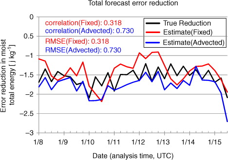
First, the effect of incorporating a moving localisation on the observation impact estimates is examined. Figure 1 shows the time series of the actual total forecast error reduction verified against its own analysis compared to estimates using a fixed localisation and a moving localisation. The error reduction is generally larger at 00 and 12 UTC than at 06 and 18 UTC because more conventional observations are available at 00 and 12 UTC. Observation impact estimates with the moving localisation capture better the diurnal cycles than that with the fixed localisation: the correlations and RMSEs (biases) of total impact estimates to the true forecast error reduction are 0.318 and 0.350 J kg⁻¹ (+0.144 J kg⁻¹) with the fixed localisation and 0.730 and 0.279 J kg⁻¹ (−0.212 J kg⁻¹) with the moving localisation. The average impact estimation is larger for the moving localisation than the fixed localisation and slightly larger than the actual impact. The results suggest that the estimation with moving localisation fits the actual observation impacts better than the fixed localisation.

Fig. 1 Time series of the total forecast error reduction of each estimate (unit: J kg⁻¹). Black, red and blue lines show the actual forecast error reduction verified against the own analysis, estimated error reduction from the EnKF-based method with fixed localisation (fixed) and with moving localisation (advected). Numbers on upper left corner show the correlation and RMSE of each estimate to the actual forecast error reduction.

As suggested by Kalnay et al. (2012), special attention is required on the localisation on the ensemble-based observation impact estimates. Although our approach is very simple and may not be optimal, the moving localisation applied in this experiment works well during our real data assimilation trial. More sophisticated localisation methods such as accounting for group velocity, dissipation or an adaptive localisation approach (Anderson, 2007; Bishop and Hodyss, 2009a, 2009b) may further improve the estimate. Application of the localisation is a trade-off between the signal and sampling noise. The optimisation of localisation function within the observation impact estimation should be a future research topic. In the following sections, only the results with the moving localisation are shown.

The estimation with moving localisation (−1.95 J kg⁻¹ on average) is generally larger than the actual forecast error reduction (−1.64 J kg⁻¹ on average). The estimation is also larger in terms of the standard deviation of the case-to-case variation (0.36 J kg⁻¹ for the estimate and 0.26 J kg⁻¹ for the actual value). This is partly because the coefficient of the movement of localisation is tuned to produce maximum forecast error reduction estimates. Also, the current NCEP operational EnKF system applies the covariance inflation just after the analysis update. This inflation magnifies the analysis covariance in eq. (5) and results in magnifying the Kalman gain in the impact estimation compared to that used in the EnKF analysis. This, in turn, would magnify the observation impact estimation compared to the actual impacts in the EnKF. In contrast, the adjoint-based study of Langland and Baker (2004) indicates consistently smaller estimates than the actual forecast error reductions derived from nonlinear model integration due to the lack of moist physics in the adjoint model.

4.2. Estimated impacts of each observation type

Figure 2a shows the average 24-hour forecast error reduction estimates with the moist total energy contributed from each observation type during the experiment. Negative values correspond to the reduction of the forecast error due to the assimilation of the observations. All observation types except ozone retrievals are estimated to reduce the forecast error on average in this period. In the EnKF, ozone observations are assimilated with a univariate covariance, that is, only the ozone analysis is changed, with no impact on other variables at the analysis time, thus limiting the impact of the ozone observations on the forecast. For the overall impacts, AMSUA (Advanced Microwave Sounding Unit – A) shows the largest contribution to the forecast error reduction. IASI (Infrared Atmospheric Sounding Interferometer) and Aircraft are the second and the third, followed by radiosondes and AIRS (Atmospheric Infra-Red Sounder). Compared with a past adjoint-based observation impact intercomparison study (Gelaro et al., 2010), the top four basic observing systems (excluding the observing systems not assimilated in their study such as IASI and AIRS) are consistent (AMSUA, Radiosondes, Aircraft and Satellite wind observations) despite using different data assimilation systems and observations.

Fig. 2 Estimated average 24-hour forecast error reduction contributed from each observation types (moist total energy, J kg⁻¹). (a) represents the total error reduction and (b) represents error reduction per observation.

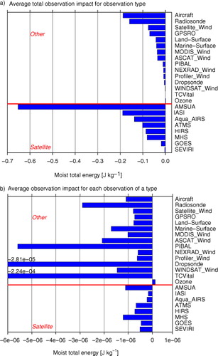
The observation impact per observation is obtained by dividing the total impact by the observation count (Fig. 2b). TCVital observations of tropical cyclones have extremely large impact per observation but the sample number is small (79 observations during the entire period and only in the Southern Hemisphere). Dropsonde observations also have very large impacts on average. Most of the dropsondes were deployed over the Northeastern Pacific during the Winter Storm Reconnaissance (WSR) program (Toth et al., 2002) led by National Oceanic and Atmospheric Administration (NOAA). This program aims to reduce the short-range forecast error of the strong extratropical cyclones using the observation targeting strategy (Bishop et al., 2001; Majumdar et al., 2002). The result suggests that this program provides valuable observations in sensitive regions and the assimilation of additional observations is effective in reducing the forecast error as expected. However, a recent OSE study (Hamill et al., 2013) reports almost neutral impact of the assimilation of WSR dropsondes to the ECMWF forecast accuracy. This discrepancy could be due to the limited sample from a single year in our study (2012). Conventional upper-air observations such as PIBAL and Radiosonde also have large impacts per observation. Satellite scatterometer winds (ASCAT_Wind and WINDSAT_Wind) and marine surface observations also have relatively large impacts. The total contributions of all of these observations to the total forecast error reduction are not large, but they are very effective per observation.

Figure 3 is a plot similar to Fig. 2 but measured using the dry total energy. Comparing with Fig. 2, the impacts of the most satellite radiance observations are substantially reduced, especially for the MHS (Microwave Humidity Sounder). PIBALs’ impact per observation is also reduced. For the MHS, this is consistent with the fact that MHS is sensitive to the atmospheric moisture. Most pilot balloons are used in India, Southeast Asia and Australia (during summer) where the atmospheric moisture is high and moist processes are relatively important. However, some observations such as GPSRO and MODIS winds have similar impacts with the moist and dry total energy indicating that they did not impact much on the moisture forecast. The GPSRO observations are selected in 1-km vertical bins up to 50 km and the largest number of assimilated observations is in the upper troposphere and the stratosphere (81% of assimilated observations are above 250 hPa). Therefore, their total impacts are relatively large in the upper layers where the atmosphere is dry (see Cucurull and Derber, 2008; Cucurull, 2010; Cucurull et al., 2013 for more details). Also, MODIS winds only cover the Arctic and Antarctic regions where the atmospheric moisture is scarce especially during the winter. MODIS winds are derived from both infrared and water vapour channels. MODIS winds derived from water vapour channels below 600 hPa are rejected by the QC so that 87% of assimilated MODIS wind observations are above 600 hPa. This limits the impact of MODIS wind observations in the lower troposphere where the moisture term becomes large in the total forecast error.

Fig. 3 Same as Fig. 2 but with the dry total energy norm (J kg⁻¹)

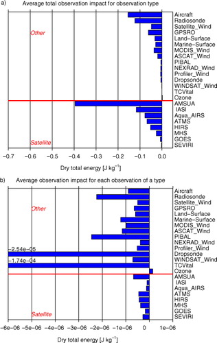
Forty-seven percent of satellite radiances and 16% of other assimilated observations are observed above 125 hPa. Although the satellite radiances have large number of observations on stratosphere compared to the other type of observations, the fractional impact of the satellite radiances is larger with the moist total energy (65%) than with the dry total energy (59%). This suggests that the impact of satellite radiance observations is especially large in the forecast of moisture.

4.3. Estimated impacts of each observation element

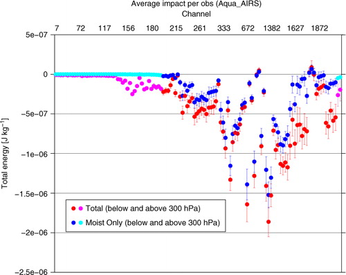
Figure 4 presents the AIRS satellite radiance impact estimates classified channel. Most of the channels have positive impact on the forecast. Some channels are estimated to have relatively large impacts, while others show small positive impacts and a few channels show small negative impacts. This information may help guide the better use of the satellite radiances through the revision of channel selection and QC method. Figure 4 also shows the estimates from only the moist term of the total energy norm. For channels 215–1627, the moist term contributes a large percentage of the total forecast impacts. These channels are mainly sensitive to the layer below 300 hPa. This suggests that these tropospheric channels are sensitive to the forecast in troposphere where the moist term of the forecast error is relatively large.

Fig. 4 Estimated AIRS satellite radiance observation impacts classified by channel with the moist total energy (red for channels sensitive below 300 hPa and magenta above 300 hPa, J kg⁻¹), and only the moist term of the total energy (blue for channels sensitive below 300 hPa and aqua above 300 hPa, J kg⁻¹). Average estimated forecast error reduction from a single observation is shown. Vertical bars represent the 95% confidence interval of the average values.

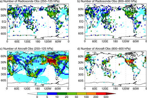
Figure 5 shows the impact of (a) RAOB and (b) aircraft per observation classified by the observation level. For the radiosonde observations, observations in the lower and middle troposphere have the largest impact on the forecast. However, aircraft observations in the lower troposphere have smaller impacts compared to the radiosonde observations. Figure 6 compares the average number of the assimilated radiosonde and aircraft observations per analysis time. Horizontal distributions of the radiosonde observations are almost the same as at 600–800 hPa and at 125–250 hPa. For the aircraft observations, the distributions are completely different. Observations at 125–250 hPa are mainly distributed over the CONUS. But they also spread widely along the major intercontinental flight tracks including over data-sparse regions such as Atlantic Ocean, Africa and Pacific Ocean. However, aircraft observations in the lower troposphere are only distributed around the airports and are much denser than the radiosonde observations. This geographical distribution of the aircraft observations in the lower troposphere and near airports that often have other conventional observations seems to limit their impacts on NWP. This suggests that the observation information in the lower troposphere around the major airports is almost saturated.

Fig. 5 Estimated average observation impacts of a) radiosonde and b) aircraft classified by observed level (moist total energy, J kg⁻¹). Average estimated forecast error reduction by a single observation is shown.

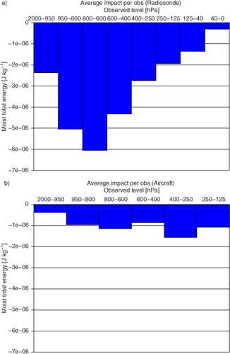
Fig. 6 Average number of assimilated radiosonde observations (a) from 250 to 125 hPa, (b) from 800 to 600 hPa and aircraft observations (c) from 250 to 125 hPa and (d) from 800 to 600 hPa in each 5°×5° area for one analysis.

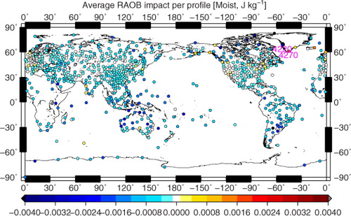
Observation impact estimates also provide the geographical distribution of the impact and relative importance of the observations. Figure 7 shows the average impacts of radiosonde per profile from fixed land stations in this experimental period. Overall, observations from most of the stations have positive impacts. Relatively large impacts are seen in the Tropics and also in Canada, Australia and South America. Large impacts in the Tropics and summer hemisphere may be a reflection of the abundance of the moisture, since the impact is evaluated with the moist total energy. By contrast, in densely observed areas such as Europe, United States and Asia, the impacts per observation are smaller. This indicates the larger importance of observations over data-sparse regions. Global observing systems may be planned to fill these gaps and meteorologically sensitive regions.

Fig. 7 Average impact (moist total energy, J kg⁻¹) of a single radiosonde profile from the fixed land stations. Only the stations that have more than 20 profiles in the period are shown. Numbers 4220 (Egedesminde) and 4270 (Narssassuaq) indicate the location of the stations shown in Fig. 8.

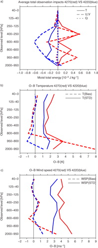
Figure 8 shows the comparison of the radiosonde observations from two neighbouring stations marked on Fig. 7 (Narssassuaq and Egedesminde, Greenland). Compared to the observations from Egedesminde, observations from Narssassuaq have large negative impact especially for temperature and wind observations on troposphere. Figure 8b and c shows the statistics of observation minus the first guess of temperature and wind speed. Both statistics show the larger standard deviation for Narssassuaq. Topography of the model surface is smoothed depending on the horizontal resolution. Surface height of the nearest GFS model grid point for this lower than operational resolution experiment is over 800 m. However, the real surface height at this point and the station height record of Narssassuaq are less than 200 m and 4 m, respectively. The area has been known as the origin of the tip jet phenomenon (Doyle and Shapiro, 1999) induced by the steep topography. This suggests that either the observations from Egedesminde are better than those from Narssassuaq or the forecast model at this resolution may not resolve a complex meteorological condition at this station. Therefore, the observations from this station may not have poor quality, but it is possible that these observations have a detrimental impact on the short-range GFS forecast by assimilating information about unresolved phenomena, giving a large error of representativeness.

Fig. 8 Comparison of the radiosonde observations from Narssassuaq (red line, 4270) and Egedesminde (blue line, 4220) showing (a) average impacts (J kg⁻¹) of each observation element (solid: temperature, dashed: winds, dotted: humidity) on each pressure level by one profile and observation departure statistics (dashed: bias, solid: standard deviation) of (b) temperature (K) and (c) wind speed (m s⁻¹).

5. Estimation and attribution of short-range regional forecast failures

The operational NWP forecasts sometimes make large forecast errors despite their relatively high average performance during short-range forecasts. For the operational NWP centres, it is critical to minimise the occurrence of such bad forecasts, and if possible take corrective measures. Observation impact estimates may help find a possible cause of large short-range forecast errors in some of the cases.

To explore this potential use, local 24- and 30-hour forecast errors with the moist total energy norm were computed over rectangular latitude and longitude areas. Their latitude width is 30° and their longitude width varies with latitude so that they are almost equal area for all latitudes (Table 2). The area slides with 10° increments for latitude and 5° increments for longitude covering the whole globe. Local forecasts within a lat/lon box were identified as failures if the following two conditions were satisfied: (1) The 24-hour forecast error was larger than 1.7 times its time average and (2) the 24-hour forecast error was larger than 1.2 times of the error of 30-hour forecast from the previous analysis. These criteria are created to find those cases with larger forecast error that may be impacted by the inclusion of additional observations. Table 3 shows the list of the identified cases. If the neighbouring areas on the same initial time also meet the criteria, they are considered to be the same case and only the area with the highest error times error increase is shown in the table (the number of identified areas is also shown). With these criteria, we identified seven cases of local short-range forecast failures in this period.

Table 2 Width of longitude used for the local area on each latitude band

Latitude	Width for longitude (°)
60N–90N	60
50N–80N	40
40N–70N	30
30N–60N	20
20N–50N	20
10N–40N	15
0N–30N	15
10S–20N	15

Only the values for Northern hemisphere are shown since it is symmetric in the Southern Hemisphere.

Table 3 List of local 24-hour forecast failure cases (initial time from 00 UTC, 8 January 2012, to 18 UTC 7 February 2012)

Initial	Area	Size	Rate	N	Denied observation (denied number/total number)	Change (estimate)
06 UTC JAN 12	50N–80N 145E–175W	1.99	1.36	5	AMSUA ch4, 5, 6 (2735/125 063)	−8.7% (−19.5%)
00 UTC JAN 16	30N–60N 20W–0	2.71	1.35	6	GPSRO 600–950 hPa (50/4918)	−0.6% (−4.3%)
18 UTC JAN 27	30S–0 105E–120E	2.40	1.21	1	AIRS (19 908/670 041)	−0.2% (−6.0%)
00 UTC JAN 30	70S–40S 165E–165W	2.00	1.25	6	AMSUA ch1, 3, 4, 5, 15 (3822/164 934)	−4.7% (−12.8%)
06 UTC FEB 2	50N–80N 150W–110W	3.01	1.22	5	GPSRO 250–400 hPa, 600–850 hPa (407/13 092)	−11.7% (−8.7%)
06 UTC FEB 4	30N–60N 150W–130W	1.81	1.26	3	IASI (57 950/1 177 256), HIRS ch3, 4, 9, 11, 12, 14, 15 (785/73 419), Aircraft 950 hPa~, 125–600 hPa (5794/100 896)	−25.5% (−81.6%)
18 UTC FEB 6	60N–90N 40E–100E	1.71	1.38	2	MODIS_Wind (10 970/43 452)	−28.4% (−47.7%)

The third, fourth and fifth columns show the forecast error size normalized with the time-averaged error, the rate of the error size compared with the error of 30-hour forecast from the previous analysis, and the number of areas that meet the criteria. Sixth column shows the denied observation type based on the observation impact estimates, number of denied observations and total number of observations with this observation type assimilated in the original analysis. Finally, seventh column shows the change of the 24-hour local forecast error for observation denial experiment and corresponding estimated forecast error change in the parenthesis. The case shown in bold font is the example shown in Fig. 9.

For each of these local forecast failures, we identify the observations that may have caused the failure. The candidate observations are selected as follows: First, the observation type estimated to have the largest negative impact is selected. In addition, any observation types estimated to have produced more than half of the total forecast degradation are also selected. Next, vertical levels (channels for satellite radiance and eight vertical levels for other observation types) are selected from the vertical level of the largest negative impact to that of the smallest until the summed impact reaches 100% of the total impact of the selected observation types. Also, the vertical levels in which observations have more than half of the total negative impact are selected. Finally, observations in local 10°×10° areas are selected for each selected observation type and vertical level whose average absolute impact is larger than 10% of maximum average absolute impact on that vertical level and observation type. The analysis and the 24-hour forecast are then reprocessed without the selected observation sets. Table 3 also shows the denied observations, their number compared to the number of all assimilated observations of the specific observation type, and the change of the 24-hour forecast error in the data-denial experiment and its estimate. The local forecast errors are in fact reduced in all seven cases by the observation denial. The forecast error estimations are larger than the actual forecast error reduction amounts in all but one case. The removal of certain set of observation can change the basic fields that are used for the linear estimation. This implies that these nonlinear effects could reduce the observation impact compared to the linear estimation.

The left panel of Fig. 9 shows the 24-hour forecast error of 500 hPa geopotential height around the Arctic region from the original analysis on 18 UTC 6 February 2012. There is a large forecast error associated with the trough over the Russian Arctic coast. Figure 9 (middle panel) also shows the forecast change due to the removal of the MODIS polar wind observations in the data-denial experiment. The forecast error of this trough is made larger by the assimilation of the MODIS polar winds observations, validating the observation impact estimates. There are several possible factors that could have made the forecast worse with the inclusion of the MODIS wind observations. For example, MODIS winds are derived from the tracking of clouds whose height is sometimes uncertain. Height assignment of the atmospheric motion vector in polar region is especially difficult (Key et al., 2004) and this may affect the assimilation of the MODIS winds.

Fig. 9 Twenty-four hour forecast error of 500 hPa geopotential height (unit: m, 18 UTC 6 February 2012 initial) from original analysis (left) and forecast change due to the removal of the MODIS polar wind observations in the data-denial experiment (middle: actual change and right: projection on the ensemble perturbations). Black contours show the analysis. Magenta cones show the target area of the observation impact estimate.

The right panel of Fig. 9 shows the estimated forecast change with and without MODIS wind observations. Substituting the observational increment of the denied observations to , eq. (8) is used to estimate the forecast change. This example indicates that eq. (8) indeed captures quite well the actual forecast change, validating the approximation in eqs. (6) and (8). Projection on the ensemble perturbations like eq. (8) should be very useful especially when the size of the partial observation set is small.

6. Summary and discussion

Observation impact estimates within the GFS/EnKF have been investigated using the formulation of Kalnay et al. (2012). A simple moving localisation based on the average wind has been applied to the impact estimates. Although it is not optimal, this method seems to work well. Assimilating all observations used in the operational global analysis (except for TRMM/TMI precipitation retrievals), the observation impacts are estimated for each observation type. Satellite radiance observations are estimated to be most important in reducing the short-range forecast error especially for moisture. However, other observations such as aircraft observations, radiosonde, marine surface observations and scatterometer winds also have high value, and the last two observation types have especially large impacts when the impacts per observation are measured.

Classified with the observation types and conditions, some examples of the advantages and disadvantages of each observing system are shown. Aircraft observations in the lower troposphere have smaller impacts per observation than the radiosondes probably because of their abundance near major airports, so that they are less evenly distributed than radiosondes stations. Estimated impacts of AIRS channels show large positive impacts on the moisture and dynamical variables for many channels, and small negative impacts for a few moisture channels, indicating that the radiances may not be optimally assimilated. Such information may guide the improvement of the use of observations in the data assimilation and possibly the design of the observation network. Continuous monitoring like Naval Research Laboratory (NRL) and National Aeronautics and Space Administration/Global Modeling and Assimilation Office (NASA/GMAO) do with the adjoint-based impact estimates may be beneficial in the operational NWP system to detect the assimilated observations that are not optimally assimilated.

We developed simple criteria to detect cases of ‘short-range regional forecast failures’, indicating that the 24-hour forecast is significantly worse than average, and worse than the 30-hour forecast started 6 hours earlier, that is without using the observations assimilated at the initial time. An analysis of cases of local short-range forecast failure indicates that these observation impact estimates can be used as a tool to identify those observations that may have caused the large forecast errors. The projection of the observational innovation on the forecast change agrees well with the corresponding data-denial experiment, validating the approximation made on the formulation of the observation impact estimates. We note that identifying short-range (12 or 24 hours) forecast failures would make possible a more ‘proactive’ QC approach where poor observations are withdrawn and the analysis recomputed in time to improve more long-range forecasts. Although the current operational global data assimilation system in NCEP cannot use this approach due to time constraints, such early identification of flawed observations may also guide studies to improve the algorithms with which they are generated or quality controlled.

Acknowledgements

The authors thank Daryl Kleist (NCEP/EMC) for valuable discussion and his continuous encouragement of this work, and Dr. Mitch Goldberg for his support of this research. Jeff Whitaker (NOAA/ESRL) first developed the EnKF data assimilation system used in this study. Discussions with Ricardo Todling (NASA/GMAO) helped us to understand better this method. The authors are grateful to two anonymous reviewers for their thoughtful comments and suggestions that helped us improve the manuscript. This work was partially supported by a NESDIS/JPSS JPSS Proving Ground (PG) and a Risk Reduction (RR) CICS Grant.

8. Appendix

Ancell and Hakim (2007) proposed to use ensemble sensitivity method to estimate the impact of additional observations using ensembles. Equation (28) in their paper can be expressed as following using the notation applied in this article,A1

where B is the background error covariance and D consists of its diagonal elements. J is any scalar forecast error metric and is its ensemble sensitivity to the first guess defined by eq. (13) in their paper. Note that the original eq. (28) is missing the transpose on the first bracket and A (initial error covariance) in eq. (28) should be interpreted as B in our discussion since we try to estimate the impact of the observations already assimilated. Equation (A1) can be modified using eqs. (11) and (14) in their paper:A2

where J is the ensemble perturbation of forecast error metric J (1 by number of ensemble member matrix). If the Kalman gain matrix is expressed with background error covariance instead of analysis error covariance, eq. (8) can be reformulated as,A3

where the approximation is used instead of . Comparing eqs. (A2) and (A3), eq. (8) can be equivalent to ensemble sensitivity method in Ancell and Hakim (2007) provided that estimation is done for additional observations and a scalar error metric is used instead of the actual forecast field.

References

- Ancell A , Hakim G. J . Comparing adjoint- and ensemble-sensitivity analysis with applications to observation targeting. Mon. Wea. Rev. 2007; 135: 4117–4134.
- Anderson J. L . An ensemble adjustment Kalman filter for data assimilation. Mon. Wea. Rev. 2001; 129: 2884–2903.
- Anderson J. L . Exploring the need for localization in ensemble data assimilation using a hierarchical ensemble filter. Physica. D. 2007; 230: 99–111.
- Bishop C. H , Etherton B. J , Majumdar S. J . Adaptive sampling with the ensemble transform Kalman filter. Part I: theoretical aspects. Mon. Wea. Rev. 2001; 129: 420–436.
- Bishop C. H , Hodyss D . Ensemble covariances adaptively localized with ECO-RAP. Part 1: tests on simple error models. Tellus A. 2009a; 61: 84–96.
- Bishop C. H , Hodyss D . Ensemble covariances adaptively localized with ECO-RAP. Part 2: a strategy for the atmosphere. Tellus A. 2009b; 61: 97–111.
- Bouttier F , Kelly G . Observing-system experiments in the ECMWF 4D-Var data assimilation system. Q. J. Roy. Meteorol. Soc. 2001; 127: 1469–1488.
- Cardinali C . Monitoring the observation impact on the short-range forecast. Q. J. Roy. Meteorol. Soc. 2009; 135: 239–250.
- Cucurull L . Improvement in the use of an operational constellation of GPS radio occultation receivers in weather forecasting. Wea. Forecast. 2010; 25: 749–767.
- Cucurull L , Derber J. C . Operational implementation of COSMIC observations into NCEP's global data assimilation system. Wea. Forecast. 2008; 23: 702–711.
- Cucurull L , Derber J. C , Purser R. J . A bending angle forward operator for GPS radio occultation measurements. J. Geophys. Res. 2013; 118: 14–28.
- Doyle J. D , Shapiro M. A . Flow response to large-scale topography: the Greenland tip jet. Tellus A. 1999; 51: 728–748.
- Ehrendorfer M , Errico R. M , Raeder K. D . Singular-vector perturbation growth in a primitive equation model with moist physics. J. Atmos. Sci. 1999; 56: 1627–1648.
- Gaspari G , Cohn S. E . Construction of correlation functions in two and three dimensions. Q. J. Roy. Meteorol. Soc. 1999; 125: 723–757.
- Gelaro R , Langland R. H , Pellerin S , Todling R . The THORPEX observation impact intercomparison experiment. Mon. Wea. Rev. 2010; 138: 4009–4025.
- Hakim G. J , Torn R. D . Ensemble-based sensitivity analysis. Mon. Wea. Rev. 2008; 136: 663–677.
- Hamill T , Yang F , Cardinali C , Majumdar S . Impact of targeted winter storm Reconnaissance dropwindsonde data on mid-latitude numerical weather predictions. Mon. Wea. Rev. 2013; 141: 2058–2065.
- Hunt B. R , Kostelich E. J , Szunyogh I . Efficient data assimilation for spatiotemporal chaos: a local ensemble transform Kalman filter. Physica. D. 2007; 230: 112–126.
- Kalnay E , Ota Y , Miyoshi T , Liu J . A simpler formulation of forecast sensitivity to observations: application to ensemble Kalman filters. Tellus A. 2012; 64: 18462.
- Key J. R , Santek D , Velden C. S . Atmospheric motion vector height assignment in the polar regions: issues and recommendations. Proceedings of 7th International Winds Workshop. 2004; EUMETSAT, Helsinki, Finland
- Kunii M , Miyoshi T , Kalnay E . Estimating impact of real observations in regional numerical weather prediction using an ensemble Kalman filter. Mon. Wea. Rev. 2012; 140: 1975–1987.
- Langland R. H , Baker N. L . Estimation of observation impact using the NRL atmospheric variational data assimilation adjoint system. Tellus A. 2004; 56: 189–201.
- Li H , Liu J , Kalnay E . Correction of ‘estimating observation impact without adjoint model in an ensemble Kalman filter’. Q. J. Roy. Meteorol. Soc. 2010; 136: 1652–1654.
- Liu J , Kalnay E . Estimating observation impact without adjoint model in an ensemble Kalman filter. Q. J. Roy. Meteorol. Soc. 2008; 134: 1327–1335.
- Majumdar S. J , Bishop C. H , Etherton B. J , Toth Z . Adaptive sampling with the ensemble transform Kalman filter. Part II: field program implementation. Mon. Wea. Rev. 2002; 130: 1356–1369.
- Toth Z , Szunyogh I , Bishop C , Majumdar S , Morss R , co-authors . Adaptive observations at NCEP: past, present, and future. Proceedings of the Symposium on Observations, Data Assimilation, and Probabilistic Prediction. 2002; January. 13–17 Boston, USA: American Meteorological Society.
- Whitaker J. S , Hamill T. M . Ensemble data assimilation without perturbed observations. Mon. Wea. Rev. 2002; 130: 1913–1924.
- Whitaker J. S , Hamill T. M , Wei X , Song Y , Toth Z . Ensemble data assimilation with the NCEP global forecast system. Mon. Wea. Rev. 2008; 136: 463–482.
- Zapotocny T. H , Jung J. A , Marshall J. F. L , Treadon R. E . A two-season impact study of satellite and in situ data in the NCEP Global Data Assimilation System. Wea. Forecast. 2007; 22: 887–909.
- Zapotocny T. H , Jung J. A , Marshall J. F. L , Treadon R. E . A two-season impact study of four satellite data types and rawinsonde data in the NCEP Global Data Assimilation System. Wea. Forecast. 2008; 23: 80–100.
- Zhu Y , Gelaro R . Observation sensitivity calculations using the adjoint of the Gridpoint Statistical Interpolation (GSI) analysis system. Mon. Wea. Rev. 2008; 136: 335–351.
8. Appendix
Ancell and Hakim (Citation2007) proposed to use ensemble sensitivity method to estimate the impact of additional observations using ensembles. Equation (28) in their paper can be expressed as following using the notation applied in this article,A1