Relationships between convective asymmetry, imbalance and intensity in numerically simulated tropical cyclones

Abstract

This article examines the relationships between convective asymmetry (CA), imbalance and intensity in tropical cyclones (TCs) that emerge from random winds on the periodic f-plane in a cloud-system-resolving numerical model. The model is configured with warm-rain microphysics and includes a basic parameterisation of long-wave radiation. Within the simulation set, the sea-surface temperature ranges from 26 to 32°C, and the Coriolis parameter f ranges from 10⁻⁵ to 10⁻⁴ s⁻¹. The number of TCs that develop in a simulation increases rapidly with f and ranges from 1 to 18. Taken together, the simulations provide a diverse spectrum of vortices that can be used for a meaningful statistical study.

Consistent with earlier studies, mature TCs with minimal asymmetry are found to have maximum wind speeds greater than the classic theoretical value derived by Emanuel under the assumptions of gradient-wind and hydrostatic balance. In a statistical sense, it is found that the degree of superintensity with respect to balance theory reliably decays with an increasing level of inner-core CA. It is verified that a more recent version of axisymmetric steady-state theory, revised to incorporate imbalance, provides a good approximation for the maximum (azimuthally averaged) azimuthal wind speed V _max when CA is relatively weak. More notably, this theory for axisymmetric vortices maintains less than 10% error as CA becomes comparable in magnitude to the symmetric component of inner-core convection. Above a large but finite threshold of CA, axisymmetric steady-state theory generally over-predicts V _max. The underachievement of TCs in this parameter regime is shown to coincide with substantial violation of the theoretical assumption of slantwise convective neutrality in the main updraft of the basic state. Of further interest, a reliable curve-fit is obtained for the anticorrelation between a simple measure of CA and V _max normalised to an estimate of its balanced potential intensity that is based solely on environmental conditions and air–sea interaction parameters. Sensitivity of results to the surface-flux parameterisation of the numerical model is briefly discussed.

• hurricane structure
• atmospheric convection
• tropical meteorology
• planetary vortices
• modelling

1. Introduction

1.1. Background

Current understanding of tropical cyclone (TC) intensity is largely based on the influential steady-state theory of Emanuel (1986) and subsequent refinements (E86; Emanuel, 1988; Emanuel, 1995; Bister and Emanuel, 1998; Emanuel and Rotunno, 2011). Consistent with earlier studies, Emanuel's theory stresses the critical role of latent and sensible heat transfer at the air–sea interface in maintaining the circulation (cf. Malkus and Riehl, 1960; Riehl, 1963; Ooyama, 1969, 1982). The importance of this transfer is reflected in a succinct analytical expression for the maximum azimuthal wind speed V _max that increases with the magnitude of air–sea disequilibrium (see Section 3). Despite the well-recognised merits of E86, its analytical framework involves several approximations whose deficiencies are gradually coming to light [Persing and Montgomery, 2003; Montgomery et al., 2006; Smith et al., 2008; Bryan and Rotunno, 2009a, b (BR09a,b); Montgomery et al., 2010; Bryan, 2012a,b]. One such approximation is gradient-wind and hydrostatic balance. Another more basic approximation is symmetry about the central axis of rotation.

The possibility for significant violation of the balance assumption has been clearly shown in numerical simulations of axisymmetric TCs (e.g. BR09b). In these simulations, supergradient flow develops near the radius of maximum wind (RMW) and creates a condition of ‘superintensity’, in which V _max exceeds the value given by balanced steady-state theory. Bryan and Rotunno (BR09b) recently revised the classic theoretical formula for V _max to permit gradient-wind and hydrostatic imbalance, and showed that their revision accurately accounts for superintensity in many simulated hurricanes. Nevertheless, the revised theory of BR09b does not directly address the potential impact of asymmetry.

The assumption of an axisymmetric vortex is violated to some degree in all natural and realistically simulated TCs. Whether the asymmetric perturbations are associated with intrinsic fluctuations or external forcing, modelling studies typically show that non-axisymmetric TCs have weaker intensity than their axisymmetric counterparts (Frank and Ritchie, 2001; Yang et al., 2007; Riemer et al., 2010; Bryan, 2012a; Persing et al., 2013). In some cases, the weakening may be connected to the enhanced flux of low-entropy air into the convective core of the vortex (cf. Tang, 2010; Tang and Emanuel, 2010, 2012). One might also speculate that convective asymmetry (CA) weakens a TC partly by inhibiting the imbalance associated with superintensity, in loose analogy to the suppression of imbalance that is typically found upon increasing parameterised eddy-diffusivity in a numerical model (cf. Fig. 12 of BR09b).

1.2. Overview of this study

This study aims to improve current quantitative knowledge of the relationships between inner-core CA, imbalance and V _max in numerically simulated TCs. To begin with, a statistical connection is sought between the degree of CA and the deviation of V _max from its theoretical value derived under the assumptions of gradient-wind and hydrostatic balance. It will be shown that the degree of superintensity with respect to balance theory decreases in a fairly regular manner with increasing CA. It will be verified that the more general axisymmetric steady-state theory of Bryan and Rotunno (BR09b) largely accounts for superintensity and provides a good approximation for V _max when CA is relatively weak. More surprisingly, good agreement with axisymmetric steady-state theory will be found to persist as CA becomes comparable in magnitude to the symmetric component of inner-core convection. Nevertheless, there exists a threshold of CA, above which axisymmetric steady-state theory generally over-predicts V _max. The underachievement of TCs in this parameter regime will be shown to coincide with substantial violation of the theoretical assumption of slantwise convective neutrality (SCN) in the main updraft of the basic state.1 The preceding results will be discussed further in Section 6.

On another front, a reliable curve-fit is sought for the anticorrelation between a simple measure of TC asymmetry and V _max normalised to a classic estimate of its balanced potential intensity (found in E86) that is based solely on environmental conditions and air–sea interaction parameters. It is worth remarking that the existence of a reliable curve-fit using a simple asymmetry variable is not a foregone conclusion, given that standard satellite-based intensity estimates involve relatively complex, multivariable algorithms (e.g. Velden et al., 2006). Here, a number of alternatives will be considered, and it will be shown that a dimensionless measure of the precipitation asymmetry works best.

The TCs considered for this study are generated by a conventional cloud-system-resolving (CSR) numerical model on the periodic f-plane. A diverse set of TCs is ensured by initialising the simulations with a pseudo-random wind field and by using a broad range of values for both the sea-surface temperature T _s and the Coriolis parameter f. In general, each simulation produces multiple TCs. The inner-core CA of an arbitrary TC may readily develop through intrinsic fluctuations. Other factors affecting CA in a multi-vortex system may include shear in the local background flow and asymmetries in the surrounding moisture fields.

It is relevant to note that similar periodic f-plane simulations have been carried out before with GCM-like models, CSR models and simple three-layer models [Held and Zhao, 2008 (HZ08); Schecter and Dunkerton, 2009; Schecter, 2010, 2011; Khairoutdinov and Emanuel, 2012 (KE12)]. The aforementioned computational studies focused on relating TC intensity, size and frequency to environmental parameters after radiative convective equilibrium (RCE) is achieved. The present simulations generally terminate before reaching RCE, but the relatively short simulation time (9–19 d) is sufficient for the TCs to reach peak intensity and settle into mature states. In a number of cases, the mature TCs slowly evolve with time. The slow evolution beneficially broadens the spectrum of states that one may include in a statistical survey.

1.3. Outline of the remaining sections

The remainder of this article is organised as follows. Section 2 provides an overview of the numerical simulations. Section 3 reviews several theoretical expressions for the maximum wind speed of an axisymmetric, steady-state TC. Section 4 discusses the primary variable that is used to measure inner-core CA in this study. Section 5 presents the statistical relationships between CA, imbalance and intensity found in the present simulation set. Section 6 summarises and discusses the results. Appendix A provides details on the numerical algorithm used to identify TCs and measure their properties in multi-vortex simulations.

2. Overview of the numerical simulations

2.1. Basic configuration of the Regional Atmospheric Modelling System

The numerical simulations are conducted with the Regional Atmospheric Modelling System (RAMS 6.0), which was originally developed at Colorado State University and is currently distributed to the public by ATMET LLC (Cotton et al., 2003). RAMS is a state-of-the-art weather research model with a variety of options for parameterising cloud microphysics, radiation, turbulent diffusivity and surface fluxes. For this study, RAMS is configured with single-moment warm-rain microphysics (Walko et al., 1995) and a long-wave radiation scheme based on the Mahrer and Pielke (1977) model. The warm-rain microphysics configuration activates only two species of hydrometeors (cloud droplets and rain), and the Mahrer–Pielke radiation scheme neglects the effects of condensate. The turbulent diffusivity is anisotropic and is obtained from a local Smagorinsky (1963) closure with Lilly (1962) and Hill (1974) modifications.

The surface-flux parameterisation in this study is simplified from the standard formulation in RAMS (Louis, 1979; Walko et al., 2000) to one closely resembling that used in the classic TC modelling study of Rotunno and Emanuel (1987; cf. Schecter, 2011). Equations of the following form are used for the surface fluxes of horizontal momentum (τ _ux , τ _uy ), sensible heat (τ _θ ) and moisture (τ _q )1

in which u≡(u _x , u _y ) is the horizontal velocity, θ is the potential temperature, and q is the water vapour mixing ratio. The variables θ _s and q _{s *} denote θ and the saturation value for q at the sea surface. The subscript ‘ +’ indicates that the variable is evaluated at the first vertical grid point above sea level. The dimensionless surface-exchange coefficients are generally obtained from Deacon's formula2

with given in m s⁻¹. It is known today that the right-hand side (rhs) of eq. (2) is inaccurate at hurricane strength wind speeds, and that C _D ≠C _E (Black et al., 2007; Bell et al., 2012). It is reasonable to expect some difference in hurricane structure when using a more realistic surface-flux parameterisation or boundary layer scheme (cf. Braun and Tao, 2000; Smith et al., 2009; Smith and Thomsen, 2010; Bryan, 2012a). A brief discussion of this issue is deferred to Section 5.4.

The simulations are conducted on a 4000×4000 km² periodic f-plane. To accommodate the large horizontal domain on a single grid, which is required (in practice) for multi-vortex simulations, the grid resolution is roughly half that which is commonly used for isolated TC simulations. The vertical grid consists of 33 elements that are continuously stretched from 200 to 900 m to 1.8 km at altitudes of 0, 10 and 23 km above sea level. The horizontal grid spacing is 3.9 km. Rayleigh damping is applied to velocity and θ perturbations at high altitudes to suppress upward propagating waves that would otherwise remain artificially trapped in the system. The damping rate increases linearly with height z, from 0 at z=z _d to v _d at z=23 km (the model top). The values of v _d range from 3.3–6.7×10⁻³ s⁻¹, and the values of z _d are specified below.

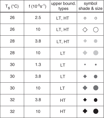
The data points appearing in this study are derived from seven low-top (LT) and five high-top (HT) simulations. The qualifier LT/HT refers to the relatively low/high altitude of the base of the damping layer (z _d=16 km or 20 km). A simulation is further characterised by its settings for the constant sea-surface temperature T _s and Coriolis parameter f. The values of T _s range from 26 to 32°C, and the values of f range from 1.3×10⁻⁵ to 10⁻⁴s⁻¹. Because a low damping layer could substantially reduce the height of the TC outflow layer over a very warm ocean, only HT simulations are considered for T _s=32°C.

Figure 1 summarises the simulation set and provides a legend of symbols that will be used in scatter plots of the data. The shade and size of a symbol indicate the values of T _s and f. Darker symbols represent simulations with higher values of T _s, and larger symbols represent simulations with higher values of f. The significance of the symbol shape (which is not necessarily a circle or diamond) depends on the particular scatter plot.

Fig. 1 Summary of the simulation set, and key to the scatter plots in this article (Figs. 4a, 4b, 8b, 9, 10, 12–14). The right-most column shows the shade and relative size of symbols used for simulations with parameters given to the left.

2.2. Initial conditions

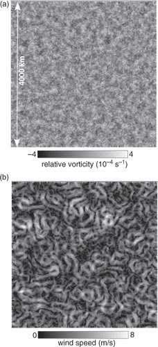
In all simulations, the ambient temperature and water vapour distributions are initialised with the Jordan (1958) mean sounding for hurricane season in the West Indies. The ambient pressure field has a surface value of 1015 hPa and satisfies the hydrostatic balance equation aloft. The lower troposphere is initialised with a non-divergent, pseudo-randomly generated horizontal velocity field u _r (Fig. 2). The velocity vector u _r is constant with increasing height until it abruptly drops to zero at z=6 km. The maximum and root mean square (rms) values of are 8.0 and 2.5 m s⁻¹, respectively. The power spectrum of u _r is proportional to k ⁻³ for horizontal wavelengths (2π/k) between 25 and 500 km, and is zero for all other wavelengths. The domain-averaged relative vorticity associated with u _r is zero. The perturbation Exner function (the prognostic pressure variable) is initialised to satisfy a partial differential equation (PDE) that ensures at t=0 for the specific case in which f=10⁻⁴s⁻¹ (cf. Appendix B of Schecter, 2011). Here, ∇ _h denotes the horizontal gradient operator. The virtual potential temperature field is slightly adjusted to ensure an initial state of hydrostatic balance. To be clear, the random velocity field is created just once, and the initial conditions for each field are the same in every simulation.2

Fig. 2 The initial wind field. (a) Relative vorticity and (b) wind speed in the horizontal plane at an arbitrary altitude below z=6 km.

2.3. Synopsis of the simulated TCs

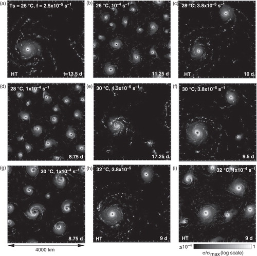
Figure 3 shows selected snapshots of the z-integrated rain mass density σ in 9 out of the 12 simulations. The values of T _s, f and the time t of the snapshot are printed on each plot. In general, these snapshots depict a state of the atmosphere past the point at which the strongest TC reaches peak intensity. In some cases, the TCs have experienced partial decay and desymmetrisation (e.g. Fig. 3g). Overall, the simulation set generates a diverse spectrum of TCs with various degrees of asymmetry.

Fig. 3 (a)–(i) Snapshots of the vertically integrated rain mass density (σ) in 9 out of the 12 primary simulations used for this study. The value of σ is normalised to the maximum value in the snapshot. The sea-surface temperature T _s and Coriolis parameter f are printed on the upper edge of each panel, whereas the time of the snapshot (in days) is printed on the bottom edge. High-top simulations are labelled with an HT on the bottom-left corner.

Figure 4a shows the f-dependence of the number of TCs N _v that develops in each simulation. The error bars are due to the decay of N _v with time (after reaching its peak value) in a few simulations. The rapid growth of N _v with increasing f is agreeable with empirical evidence suggesting that regions of elevated absolute vorticity are more favourable to TC development (e.g. Emanuel and Nolan, 2004; Camargo et al., 2007). It is also consistent with the RCE states of HZ08 and KE12. Note that the growth of N _v with the Coriolis parameter for f≥2.5×10⁻⁵ s⁻¹ seems closer to quadratic than to linear or cubic. Perhaps by coincidence, quadratic scaling would be consistent with a vortex separation length l _s proportional to the Rossby deformation radius, given that the dry static stability does not vary appreciably among the simulations. Approximate quadratic scaling (with scatter about the basic trend) might also be expected if l _s were proportional to the hypothetical RCE scale V _th/f (cf. HZ08; KE12; Chavas and Emanuel, 2012), in which V _th is the theoretical maximum wind speed of a TC derived using balance approximations in E86 [cf. eq. (7) of this article].

Fig. 4 (a) Number of significant vortices (N _v) versus the Coriolis parameter f. Downward and upward pointing triangles represent data from LT and HT simulations, respectively. The dotted curves show linear and cubic growth of N _v with increasing f, whereas the solid curve shows quadratic growth. (b) Scatter plot of the maximum azimuthal wind speed V _max against the radius of maximum wind r _max in the TCs considered for statistical analysis. The diamonds and circles respectively represent data points for the strongest and median vortices defined in Section 2.4. A ‘+’ or ‘×’ behind a symbol means that the data point is taken from an HT simulation. The shading and relative size distribution of symbols in (a) and (b) are explained in Fig. 1. Each datum in (b) is a five-snapshot average, as explained in Section 4. (c) Colour contour plot of the azimuthally averaged wind speed () in a typical TC, with markers at V _max and r _max. 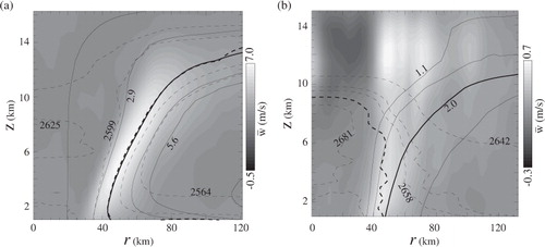Specifically, this TC is from the HT simulation with T _s=26°C and f=2.5×10⁻⁵ s⁻¹.

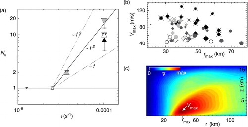
Figure 4b shows a scatter plot of the maximum azimuthal wind speed V _max against the radius of maximum wind r _max for mature TCs in all of the simulations. Data for both the strongest and median-strength TCs in a given simulation are shown, as these vortices will be the focus of the forthcoming statistical analysis. Different data points for the same (statistically defined) TC are taken at different times after peak intensity is achieved. The values for V _max range from minimal hurricane strength to unnaturally high magnitudes that exceed 120 m s⁻¹. The values of r _max range from 20 to 80 km and are not strongly correlated to V _max. For illustrative purposes, Fig. 4c shows the location of V _max in a vertical cross-section of a typical TC. Section 5.3 will address the extent to which environmental parameters control the value of V _max in the present simulation set. It is worth noting that environmental control over r _max seems minimal. At best, r _max may have a weak positive correlation with f and a weak negative correlation with T _s at the specific time of peak vortex intensity.

Figure 5 shows the evolution of the maximum azimuthal wind speed V _max of TCs selected from two illustrative simulations. Figure 5a corresponds to the HT simulation with T _s=32°C and f=10⁻⁴ s⁻¹. In this case, V _max exhibits considerable decay after quickly reaching its peak value.3 The decay of V _max coincides with the decay of air–sea disequilibrium as the system relaxes towards RCE. Moreover, the decay of V _max follows the dotted decay curve for the theoretical wind speed of a steady-state TC obtained from the instantaneous values of local parameters [eq. (5) of Section 3]. In other words, the evolution of the mature TC appears to be consistent with quasi-equilibrium development. Figure 5b corresponds to the HT simulation with T _s=26°C and f=10⁻⁴ s⁻¹. In this case, the TC evolves more slowly, but again follows the basic expectations of steady-state theory after achieving peak intensity.

Fig. 5 Time series of the maximum wind speed (V _max) of TCs selected from HT simulations with (a) T _s=32°C and (b) T _s=26°C. In both simulations, f=10⁻⁴ s⁻¹. The dotted curves show the maximum wind speed given by modern axisymmetric steady-state theory [i.e., V _th–l given by eq. (5)]. The time dependence of V _th–l is due to changes in local conditions that determine its value. The dotted curves begin when the nominal TC outflow altitude (z ₀ defined in Section 3) settles to within one vertical grid point of its final value. The asterisk in each plot marks the time at which sampling begins for obtaining scatter plot data from the depicted simulation.

Note that with few exceptions, the slow evolution of V _max after peak intensity coincides with slow growth of the RMW. Pertinent details on the growth rates will be discussed in Section 5.1.

2.4. Conventions for identifying and describing TCs

The vortex statistics presented in this article are obtained from snapshots taken every 6 hours (the archiving interval) in each simulation. A vortex is considered for statistical analysis only if the minimum value of its surface pressure p _s falls below a time-dependent threshold. Appendix A.1 provides details of the numerical algorithm that identifies significant vortices.

Unless stated otherwise, the central axis of the cylindrical coordinate system used to describe a TC passes through the centre of rotation x ₀ in the boundary layer. The radial, azimuthal and vertical coordinates are denoted r, ϕ and z, respectively. The corresponding unit vectors are given by , and . The radial, azimuthal and vertical velocities are denoted u, v and w. The boundary layer is here defined as the lowest part of the troposphere, extending from the sea surface to z=1 km. The vertically averaged horizontal velocity field in the boundary layer is denoted u ₀. Appendix A.2 explains how x ₀ is obtained from u ₀.

All fields within a TC are decomposed into azimuthal means and perturbations, henceforth denoted by overbars and primes. For example, the azimuthal velocity field is given by , in which . The value of V _max is equated to the maximum of . The radius and height at which are denoted r _max and z _max, respectively. The point (r _max, z _max) is generally within the lowest part of the eyewall updraft. In general, V _max is slightly greater than the maximum value of , henceforth denoted V ₀. The radius at which is denoted R ₀ and may slightly differ from r _max.

The statistical software developed for this study identifies the strongest vortex in a snapshot as that among the N _v vortices possessing the maximum of V ₀. If N _v is odd, the median vortex is that with the central value of V ₀. If N _v is even, the median vortex refers to an imaginary vortex whose measurement under consideration (such as an asymmetry variable) is the average between the two vortices with the two central values of V ₀. Note that the strongest and median vortices can change their identities with time. The strongest or median vortex is said to be in a mature state after the maximum or median value of V ₀ reaches its temporal peak, and the nominal TC outflow altitude (z _o defined in Section 3) settles to within one vertical grid point of its final value. The remaining scatter plots in this article (and Fig. 4b) show data only from mature vortices. Data points from the strongest and median vortices are deemed sufficient to convey the variability of mature TC structure in a given system. The weakest TCs are not represented in the scatter plots (when N _v≥3) because it is sometimes difficult to establish their maturity or status with respect to quasi-equilibrium.

3. Theoretical wind speed formulas

Perhaps the simplest theoretical (th) expression for the square of V _max pertinent to the simulations of this study is given by3

in which the suffix ‘lb’ in the subscript of V indicates a partial dependence on local parameters (in contrast to ambient conditions) and limited applicability to balanced vortices (E95; BR09b). The first factor on the rhs of eq. (3) reflects the intensification expected from increasing the ratio of C _E to C _D . One should bear in mind, however, that the other factors may have implicit dependencies on the surface-exchange coefficients.

The middle factor on the rhs of eq. (3) accounts for the intensification of a TC by increasing the difference between the nominal cloud-base temperature and outflow temperature T _o. Here, and in all other equations of this article, the temperatures are absolute. The value of is taken to be the ϕ-averaged temperature at (r _max, z _max). The value of T _o is obtained from the domain-averaged sounding (DAS) at the altitude z _o where the mixing ratio of small cloud droplets (q _c) is maximised. This practical estimate for T _o is reasonable only after the effect of deep convection on the z-maximum of q _c dominates that of shallow convection, and it may not have a straightforward generalisation to simulations with more complex microphysics. Figure 6 shows where z _o lies within the actual outflow of the strongest hurricanes in several of the simulations at hand.

Fig. 6 Correspondence between the TC outflow region and the altitude z _o where the horizontally averaged cloud water mixing ratio q _c(z) is peaked. (a) Shaded contour plot of the radial velocity in the r–z plane for the strongest TC in the LT simulation with T _s=28°C and f=3.8×10⁻⁵ s⁻¹ at t=10 d. The dotted curves are zero-contours of ; dark/bright shades indicate inflow/outflow. A graph of q _c (dashed curve) is superposed on the contour plot of . The values of q _c are given on the top axis. (b) Same as (a) but for the LT simulation with T _s=30°C and f=10⁻⁴ s⁻¹at t=5.25 d. (c) Same as (a) but for the HT simulation with T _s=32°C and f=10⁻⁴ s⁻¹ at t=10.5 d.

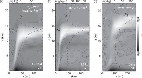
The last factor on the rhs of eq. (3) accounts for the intensification of a TC by increasing a local measure of the air–sea disequilibrium. The variables and respectively represent azimuthal averages of the saturated pseudoadiabatic entropy at the sea surface and the actual pseudoadiabatic entropy at the top of the surface layer, evaluated at r _max. The approximate formula for pseudoadiabatic entropy used here is given by4

in which c _pd is the isobaric specific heat of dry air, T is the absolute temperature, p _d is the pressure of dry air, q is the water vapour mixing ratio, is the relative humidity, R _d and R _v are respectively the gas constants of dry air and water vapour, and L ₀≡2.555×10⁶ J kg⁻¹ (Bryan, 2008).

The classic derivation of eq. (3) assumes that the TC is axisymmetric and time independent. More technical assumptions include the following:

A.1. the vortex satisfies gradient-wind and hydrostatic balance;

A.2. boundary layer air is conditionally neutral to slantwise displacements along angular momentum surfaces in the eyewall;

A.3. surface fluxes balance radial advection (of entropy and angular momentum) in the inflow layer at the base of the eyewall.

By now, it is well-known that V _th–lb can severely under-predict V _max largely due to violation of balance (A.1) near the RMW (Smith et al., 2008; BR09b). Permitting imbalance leads to the following more general theoretical wind speed formula [cf. eq. (23) of BR09b]5

in which6

The correction due to imbalance (Γ) is simply times the azimuthal vorticity of the secondary circulation, evaluated at the location of maximum wind speed. Typically, the value of Γ increases with the local degree of supergradient flow (BR09b).4

Comparing V _max to V _th–lb or V _th–l allows one to partially assess the consistency between a simulated TC and axisymmetric steady-state theory, with or without balance approximations. However, evaluating V _th–lb or V _th–l requires knowledge of secondary vortex parameters and moist-thermodynamic conditions at the base of the eyewall. In contrast, eq. (43) of E86 provides a theoretical estimate for V _max that depends only on environmental conditions and air–sea interaction parameters. The E86 formula is approximately given by7

in which L=2.5×10⁶ J kg⁻¹ is the latent heat of vaporisation (neglecting temperature variation) and R=287 J kg⁻¹ K⁻¹ is the approximate gas constant of air. The variables and are the surface values of the saturation water-vapour mixing ratio and relative humidity obtained from the DAS. The parameters and ξ are defined by8

The cloud-base temperature T _B is here approximated by the value of T at the lifting condensation level of an air parcel with relative humidity and temperature T ₊ obtained from the DAS at the first grid point above sea level. Note that T ₊ is slightly less than the sea-surface temperature T _s. The outflow temperature T _o is obtained from the DAS as described previously in connection to Fig. 6. It should be noted that eq. (7) neglects a term that appears in E86 of order , in which r _o is essentially the outer radius at which the near-surface azimuthal velocity of the TC vanishes. Such neglect causes a typical error of 1% (and a maximum error of 3%) for V _th in the simulations under consideration, assuming hexagonal closely packed vortices to estimate r _o from N _v. It should also be emphasised that DAS quantities are substituted for ambient quantities in the practical evaluation of V _th. This approach seems reasonable, assuming that the inner cores of the TCs contribute little to the domain average of an arbitrary sounding variable.

4. Convective asymmetry

Several measurements of vortex asymmetry will be considered in this article. For the time being, it suffices to focus on the following measure of inner-core CA:9

The z-integrated rain-mass density appearing in the definition of δσ was introduced earlier, and it is now precisely defined by , in which z _t is the value of z at the model top, q _r is the rain-water mixing ratio, and ρ is the mass density of the gaseous component of moist air (which adequately approximates the mass density of dry air). The maximisation operators in eq. (9) act over the radial intervals 0.5≤r/R ₀≤1.5 or 0.5≤r/R ₀≤4 when appearing in the numerator or denominator, respectively.5

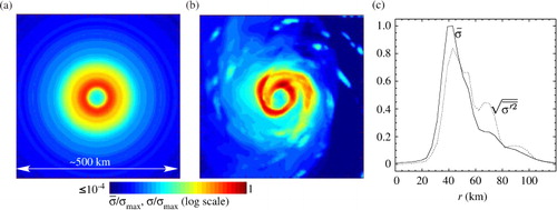
For illustrative purposes, Figure 7 shows the instantaneous rain-mass field of a TC with moderate to strong asymmetry at t=18 d in the HT RAMS simulation with T _s=26°C and f=10⁻⁴s⁻¹. Figures 7a and 7b show colour contour plots of and σ, whereas Fig. 7c shows the radial distributions of and the rms of taken along an azimuthal circuit. The maxima of the radial distributions in Fig. 7c are used in the denominator and numerator of the ratio defining δσ.

Fig. 7 Illustration of the fields used in computing the convective asymmetry variable δσ for an arbitrary TC. Plots (a) and (b) are colour contour plots of the ϕ-averaged and total z-integrated rain-mass densities and σ, respectively, normalised to the maximum of σ. Plot (c) shows the radial profiles of and normalised to max(). The RMW (in the boundary layer) is at r=35.2 km.

Figure 8a shows the time dependence of δσ in a mature TC that was tracked during one of the simulations. Here, it is seen that δσ can have order unity fluctuations over a 1-d time period. If one attempts to match the instantaneous value of δσ to that of another statistic, such as the imbalance parameter used in Section 5.1 (V _th–l/V _th–lb, dashed curve), one can obtain very different results depending on the time t. Taking V _th–l/V _th–lb=1.038±0.002, δσ can be as large as 1.08 or as small as 0.45.

Fig. 8 (a) Time series of δσ (solid curve) for a TC found in the HT simulation with T _s=26°C and f=10⁻⁴ s⁻¹. The dashed curve shows the time series of V _th–l/V _th–lb, whose difference from unity is a dimensionless measure of imbalance. The statistical relationship between δσ and V _th–l/V _th–lb is examined in Section 5.1. (b) Scatter plot of δσ against the core vertical kinetic energy asymmetry δKE_w. The solid line striking through the data points is a power-law curve-fit. The symbols are the same as in Fig. 4b.

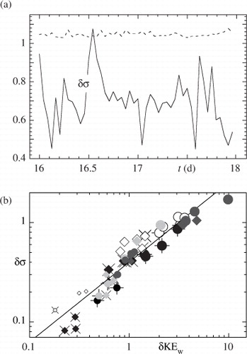
To reduce excessive scatter associated with instantaneous measurements, the statistics plotted in this article (Figs. 4b, 8b, 9, 10, 12–14) are generally averages taken from five snapshots covering a 30-hour time window. It should be remarked that a five-snapshot-average statistic for the strongest or median vortex is not necessarily obtained from a single TC, since that vortex can change its identity over time. An illustrative comparison between averaged and unaveraged data is deferred to Section 5.3 (Fig. 13a).

It is worth noting that a positive correlation is expected between δσ and other asymmetries of the secondary circulation. Figure 8b demonstrates that there is an especially strong correlation between δσ and the asymmetry of core vertical kinetic energy, defined by10

It is also worth noting that higher grid resolution may increase the value of δσ for cases in which the rain-mass asymmetry is dominated by small-scale features. Of course, all comparisons of δσ made in this article are at the same resolution.

5. Statistical connections between CA, imbalance and TC Intensity

5.1. The relationship between convective asymmetry and superintensity

Having introduced a quantitative measure of CA (δσ), it is now possible to discuss the statistical relationship between the degree of CA and the deviation of V _max from its theoretical value derived under the assumptions of gradient-wind and hydrostatic balance. Figure 9a shows that V _max generally exceeds V _th–lb for mature TCs with δσ<1. Furthermore, the degree of superintensity (V _max/V _th–lb−1) is seen to decay in a fairly regular manner with increasing δσ. A few simulations have data points that fall significantly below the main (top) decay curve. Nevertheless, when the lower simulations are considered separately, they too show that superintensity decays with increasing δσ.6

Fig. 9 Maximum wind speed V _max divided by one of two theoretical values vs. the inner-core convective asymmetry variable δσ. The theoretical wind speed V _th–lb in (a) assumes gradient-wind and hydrostatic balance. The theoretical wind speed V _th–l in (b) accounts for imbalance. Data are shown for the median and strongest vortices (after achieving peak intensity) in all simulations. The symbols are the same as in Fig. 4b (cf. Fig. 1). The top dotted line in (a) shows the decay trend for δσ<1 in most simulations. The lower dotted lines in (a) show the decay trends for two simulations that fall below the main curve. The solid horizontal line in both (a) and (b) corresponds to perfect agreement with theory. The dotted lines in (b) correspond to 10% positive and negative deviations from theory. The lightly shaded region in the lower right corner of (b) shows where δσ≥0.8 and only underachieving vortices with V _max<V _th–l exist.

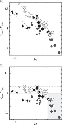
Figure 9b provides evidence that superintensity is largely due to imbalance in the simulated TCs. Specifically, Fig. 9b shows that in the domain of superintense vortices, V _max is generally within 10% of the value given by axisymmetric steady-state theory generalised to include imbalance (V _th–l). Interestingly, this high degree of accuracy persists for values of δσ up to unity.

Taken together, Figs. 9a and 9b suggest that the decay of superintensity with increasing δσ coincides with the decay of imbalance. Figure 10 verifies the implied anticorrelation between δσ and imbalance, measured by the ratio . While a causal connection cannot be inferred from an anticorrelation, the statistical decay of V _th–l/V _th–lb with increasing CA might lead one to speculate that elevated CA acts to inhibit imbalance (i.e. supergradient flow). The merit of this speculation will be assessed in Section 6, after further examination of the data.

Fig. 10 The ratio of theoretical wind speeds for unbalanced and balanced TCs (V _th–l/V _th–lb) vs. δσ. The symbols are generally the same as in Fig. 4b. However, the white plus-marks are from additional simulations with capped surface-exchange coefficients, T _s=26°C, and either f=2.5×10⁻⁵s⁻¹ (small symbol) or f=10⁻⁴s⁻¹ (large symbols).

Note that a few of the TCs with δσ<1 in Fig. 9b are anomalous in that V _max/V _th–l<0.9. Unsurprisingly, the aberrant TCs belong to the same simulations whose data points fall below the main decay curve in Fig. 9a. These simulations have additional abnormalities worth mentioning. One of the simulations at issue is the LT experiment with T _s=30°C and f=1.3×10⁻⁵ s⁻¹. In this case, the RMW of the sole TC is exceptionally small (Fig. 4b, far left), and inadequate grid resolution is a conceivable source of error. In the other two simulations, the RMWs of the mature TCs have abnormally fast growth rates. In other words, these simulations seem to violate the steady-state assumption more so than others. For the abnormal HT simulation with T _s=32°C and f=3.8×10⁻⁵ s⁻¹, the RMW growth rate (averaged over all TCs) during the last 2 days of simulation time is 6.8 km d⁻¹. For the abnormalLT simulation with T _s=30°C and f=3.8×10⁻⁵ s⁻¹, the growth rate is 13.7 km d⁻¹. For all other simulations, the RMW growth rate has an average value of 2.2 km d⁻¹ and a maximum value of 3.9 km d⁻¹.

5.2. An apparent asymmetry threshold for the integrity of axisymmetric steady-state theory

The continued decay of V _max/V _th–lb with increasing δσ beyond unity (Fig. 9a) is not attributable to a further decline of imbalance, but appears to be connected in part to the breakdown of SCN in the main updraft of the basic state.¹ Figure 11 compares the ϕ-averaged structure of a TC with δσ=0.13 and V _max/V _th–l=1.09 to that of an underachieving TC with δσ=1.4 and V _max/V _th–l=0.66. Each panel shows superposed contour plots of absolute angular momentum , saturated pseudoadiabatic entropy and vertical velocity . The congruence of M and contours in the eyewall updraft of the TC with δσ=0.13 is tantamount to SCN, and it is typical of mature TCs that have low to moderate CA. The incongruence of M and contours in the underachieving TC with δσ=1.4 indicates the violation of SCN. One reasonable measure for the violation of SCN is given by , in which is evaluated at (r _max, z _max) and is evaluated at z=6 km on the M contour passing through (r _max, z _max). The value of ɛ _SCN for the underachieving TC in Fig. 11b is 30 times greater than its value for the nearly symmetric TC in Fig. 11a.

Fig. 11 Mean structure above the inflow layer for simulated TCs with (a) δσ=0.13 and (b) δσ=1.4. The solid and dashed curves are contours of constant angular momentum (M) and saturation entropy (), sparsely labelled in units of 10⁶ m²s⁻¹ and J kg⁻¹K⁻¹, respectively. The relatively thick contours pass through the location of V _max. The shading shows the azimuthally averaged vertical velocity . The TC in (a) is the sole vortex at the end of the HT simulation with T _s=26°C and f=2.5×10⁻⁵s⁻¹. The TC in (b) is one of the median vortices near the end of the LT simulation with T _s=30°C and f=10⁻⁴s⁻¹. In both cases, the profiles are averages over five snapshots taken 6 hours apart.

While seen here only for a few TCs, it seems plausible that δσ>1 should more generally correspond to the breakdown of SCN, which is based on the supposition of purely axisymmetric, time-independent moist-convection.

5.3. Predicting wind speed from environmental conditions and the degree of asymmetry

As noted earlier, E86 provides an estimate for TC intensity [V _th given by eq. (7)] that depends only on environmental conditions and the ratio C _E /C _D (which here equals 1). It is of interest to investigate whether or not the deviation of V _max from V _th is reliably predicted by the degree of vortex asymmetry in the present simulation set. The analysis shown here includes all TCs in Fig. 9, but similar results are found using only those with .

Figure 12a demonstrates that the deviation of V _max/V _th from unity is predicted fairly well by the value of δσ. The goodness of this predictor may be compared to that of other asymmetry variables. Figures 12b–d show scatter plots of V _max/V _th against the following measures of inner-core asymmetry:11

Fig. 12 Comparison of the reliability of different asymmetry variables for predicting V _max/V _th. (a–d) Scatter plots of V _max/V _th against (a) δσ, (b) δw, (c) δu and (d) Tilt. The rain-mass asymmetry δσ is the most reliable predictor of those considered here. The symbols are the same as in Fig. 4b.

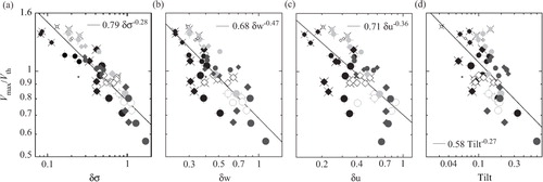
The low-level updraft asymmetry δw involves the vertical velocity w ₀(r, ϕ) at z=1 km. The radial inflow asymmetry δu involves the radial velocity u ₀(r, ϕ) defined as the vertical average of u between the sea surface and z=1 km. The Tilt is generally the horizontal distance δx ₁₂ between rotational centres x ₁ at p ₁=850 hPa and x ₂ at p ₂=200 hPa, divided by the mean RMW at these pressure levels (the mean of R _n , n∈{1,2}). The maximisation operators in eq. (11) have the same meaning as in the definition of δσ [eq. (9)]. The operands are generally maximised in the vicinity of the eyewall, but they are not necessarily maximised at the same radius. Appendix A provides some technical details on the computations of u ₀, x _n and R _n .

Visual inspection of Fig. 12 suggests that δσ is a better predictor of V _max/V _th than the alternatives given above. To state this quantitatively, the decay of V _max/V _th with each asymmetry variable is fit to a power-law using the method of least-squares. Each curve-fit is printed on the corresponding graph. The accuracy of one fit relative to another is here assessed by comparing the computed values of12

in which y _i and y _fi are the logarithms of the actual and fit values of V _max/V _th at the i-th data point, is the mean of y _i , and the sums are over all data points. The denominator in eq. (12) does not vary in this analysis. The value of Q is generally between 0 and 1, with 0 indicating a perfect fit and 1 indicating an rms deviation of y _i from the curve-fit equal to the standard deviation of y _i from its mean. It is found that Q _δσ =0.43, Q _δw =0.61, Q _δu =0.72 and Q _Tilt=0.78, in which the subscript indicates the asymmetry used as the predictor of V _max/V _th. The inferior predicting value of Tilt seems reasonable given that the pressure levels of x ₁ and x ₂ are somewhat arbitrary, and δx ₁₂ does not usually exceed a few grid increments in the simulation set at hand. It is not as obvious to the author why δw and δu are inferior to δσ, but this result may deserve further study if found to be common in future computational experiments and observational analyses.7

Of course, one cannot claim that δσ is the best of all possible predictors for V _max/V _th. Not only does δσ contain incomplete information on the structural asymmetry of the vortex, but environmental factors could affect the impact of asymmetric perturbations on vortex intensity. One conceivable hybrid predictor is δσ multiplied by the following dimensionless measure of the lower-middle tropospheric moist-entropy deficit8 13

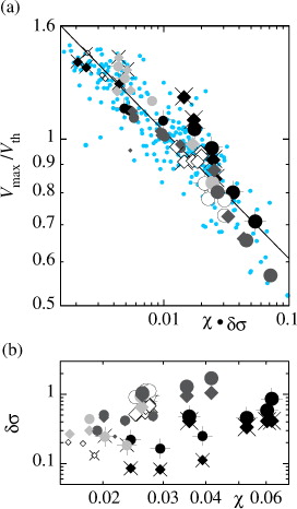
Here, s _m and s _m* are actual and saturation values of the pseudoadiabatic entropy of the DAS at p=600 hPa. Figure 13a shows a scatter plot of V _max/V _th against χ δσ. The power-law curve-fit for the anticorrelation has a normalised error of , which is a small but notable improvement over Q _δσ =0.43. It has been found that , and Tilt are also better power-law predictors of V _max/V _th than their bare counterparts (compare , and to the Q values given in the preceding paragraph). Typical improvement in the predictive value of an asymmetry variable by factoring in could be accidental, but it seems agreeable with the general notion that the flux of low-entropy air into the convective core of the storm factors into the detrimental impact of asymmetric perturbations on TC intensity.

Fig. 13 (a) Non-dimensional wind speed V _max/V _th vs. the product of the lower-middle tropospheric moist-entropy deficit and the convective asymmetry variable δσ. The curve-fit (solid line) is given by . (b) Scatter plot of δσ against . The symbols are generally the same as in Fig. 4b, but the small blue dots in (a) show instantaneous measurements as opposed to averages taken over five snapshots (white, black and grey symbols).

Figure 14 shows that in addition to its anticorrelation with V _max/V _th, the rain-mass asymmetry δσ has a fairly strong anticorrelation with the dimensional wind speed V _max in the simulation set at hand. One might liberally combine the curve-fit equation for V _max/V _th against δσ (or ) with the curve-fit equation for V _max against δσ to obtain an ad hoc equation for V _max that depends only on environmental conditions and air–sea interaction parameters. However, it is the author's opinion that the effort to accurately eliminate asymmetry from the V _max equation under general circumstances is best deferred until future theoretical work provides more guidance.

Fig. 14 Dimensional wind speed V _max versus δσ. The curve-fit (solid line) is given by in units of m s⁻¹. The symbols are the same as in Fig. 4b.

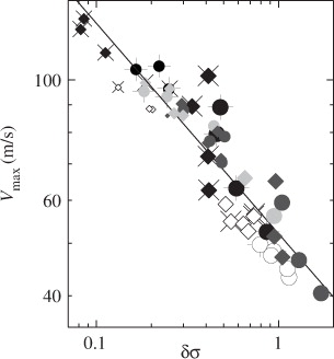
A few brief remarks are in order before proceeding to the next section. First note that the power-law curve-fits in Figs. (12–14) are not supposed to apply outside the finite bounds of asymmetry (and ) in the present data set. This is seen clearly from the unphysical divergence of V _max predicted by the curve-fits as asymmetry tends to zero. Note also that while data averaged over five snapshots is used here to quantify the decay of V _max/V _th with increasing asymmetry, the instantaneous data points (e.g. the small blue dots in Fig. 13a) typically do not stray too far from the averaged data points. A few exceptions are seen in Fig. 13a, as one might have anticipated from the discussion of Section 4 in connection to Fig. 8a. Note finally that while elevated levels of may be one cause for elevated levels of δσ, the two quantities are not strongly correlated in the present computational data set (Fig. 13b).

5.4. Comment on the surface-flux parameterisation

The anticorrelation between V _max and δσ in Fig. 14 suggests that greater imbalance at low values of δσ coincides with greater values of C _D and C _E [see eq. (2)]. One might reasonably suspect that such intensification of the surface-exchange coefficients influences the degree of supergradient flow. A comprehensive surface-flux sensitivity test is not presented in this article. However, the author has briefly examined the consequence of capping the values of C _D and C _E in the two HT simulations with T _s=26°C, by letting in eq. (2). In neither case does V _max change by more than 9%. For the simulation in which f=10⁻⁴ s⁻¹, the imbalance measured by V _th–l/V _th–lb changes by an average magnitude of 10⁻². For the simulation in which f=2.5×10⁻⁵ s⁻¹, V _th–l/V _th–lb decreases by 0.11. The greater reduction of imbalance in the latter case coincides with greater fractional growth of δσ. Returning to Fig. 10 of Section 5.1, it is seen that the anticorrelation between imbalance and δσ in the capped simulations (white plus-marks) quantitatively agrees with that found in the uncapped simulations. This result lends credence to the hypothesis that the basic anticorrelation between imbalance at the location of V _max and inner-core CA is not a peculiar artefact of the Deacon-type surface-flux parameterisation used for this study.

6. Summary and concluding remarks

In summary, this article examined the statistical relationships between inner-core CA, imbalance and TC intensity in a CSR model on the periodic f-plane. The CSR model was configured with warm-rain microphysics, a traditional parameterisation of surface fluxes [eqs. (1) and (2)], Smagorinsky-type eddy-diffusivity, and a simplified long-wave radiation scheme. The number of TCs generated in a simulation was found to increase rapidly with f, and ranged from 1 to 18. The statistics were obtained after the TCs achieved peak intensity.

The degree of CA was quantified by the parameter δσ [eq. (9)], which is a direct measure of the rain-mass asymmetry in the vicinity of the eyewall, and an indirect measure of asymmetry in the core vertical kinetic energy distribution (Fig. 8b). The statistical analysis showed that the degree of superintensity with respect to balance theory tends to decay with increasing δσ (Fig. 9a). Moreover, it was shown that the degree of imbalance at the location of maximum wind speed reliably decays with increasing δσ (Fig. 10).

A definitive interpretation of the structural anticorrelation between inner-core CA and imbalance cannot be established without further theoretical and experimental investigation. On the one hand, it seems plausible that inner-core CA would act to weaken and smooth the ϕ-averaged secondary circulation at (r _max, z _max) in such a way that reduces the pertinent measure of imbalance [Γ in eq. (6) divided by ]. On the other hand, inner-core CA is statistically related to other variables that could independently influence the degree of imbalance. For example, one must consider the anticorrelation between inner-core CA and the dimensional maximum wind speed V _max (Fig. 14). Notably, the weakening of TC wind speed decreases the surface drag coefficient C _D (not to mention ) in the CSR model used for this study. It seems reasonable to speculate that the reduction of surface drag attending the growth of inner-core CA contributes significantly to the decay of imbalance shown by Fig. 10 (cf. Montgomery et al., 2010; Bryan, 2012a).

This article also verified that the generalised axisymmetric steady-state theory of Bryan and Rotunno (BR09b) largely accounts for superintensity in simulated TCs, and provides a good approximation for V _max in the parameter regime where δσ<<1. More surprisingly, it was found that the wind speed given by this theory for axisymmetric vortices stays within 10% of V _max for values of δσ up to 1, provided that quasi-equilibrium is not strongly violated. (See Fig. 9b and the connected discussion.) It is worth noting that δσ of order unity corresponds to an asymmetry of core vertical kinetic energy (δKE_w) of the same general magnitude. Furthermore, values of δσ between 0.5 and 1 often coincide with radial inflow and/or low-level updraft asymmetries (δu and/or δw) in the same range.

Only a few data points were considered with δσ>1. Here, it was found that axisymmetric steady-state theory substantially over-predicts V _max. The underachievement of TCs in this parameter regime was shown to coincide with substantial violation of the theoretical assumption of SCN in the main updraft of the basic state (see Fig. 11b). It was speculated that δσ>1 should more generally correspond to the breakdown of SCN, which is based on the supposition of purely axisymmetric, time-independent moist-convection.¹

Furthermore, it was shown that the value of δσ is a relatively good statistical predictor of the deviation of V _max from the theoretical estimate of E86 (V _th) that depends only on environmental conditions and air–sea interaction parameters. The superior predictive value of δσ was determined upon comparison to several other measures of vortex asymmetry (Fig. 12). Interestingly, the asymmetry variables became better statistical predictors of V _max/V _th (in this data set) when multiplied by a dimensionless measure of the lower-middle tropospheric moist-entropy deficit. This result could be accidental, but it seems agreeable with the general notion that the flux of low-entropy air into the convective core of the storm factors into the detrimental impact of asymmetric perturbations on TC intensity.

It is reasonable to assume that changing the grid resolution, surface-flux parameterisation, microphysics parameterisation, turbulent diffusion scheme or radiation scheme would change details of the simulations considered in this article. For example, changing the computational configuration may well change the precise magnitudes of inner-core CA and imbalance in any given TC. However, one might hypothesise that the statistical relationship between these two quantities in a large set of reconfigured simulations would be similar to that found here. One might further hypothesise that the reconfigured simulations would exhibit the same threshold (δσ≈1) of applicability for axisymmetric steady-state theory, and a similar statistical dependence of V _max/V _th on δσ or one of its surrogates. Of course, with more realistic microphysics it might be necessary to generalise the definitions of δσ and V _th to account for ice. Regardless, the results presented in this article provide a reference point for future investigations.

Acknowledgements

The author thanks two anonymous reviewers for their constructive criticism of the original manuscript which led to numerous improvements in the final submission. This work was supported by two NSF grants: AGS-0750660 and AGS-1101713. The HT simulations were partly carried out on the Bluefire and Yellowstone supercomputers at the National Centre for Atmospheric Research (Boulder, CO, USA) and on the Gordon supercomputer at the San Diego Supercomputing Centre (San Diego, CA, USA).

Notes

1. Here and throughout this article, SCN refers to the condition in which the azimuthally averaged angular momentum and saturated pseudoadiabatic entropy contours are congruent.

2. A few tests suggested that adjusting the PDE for to ensure at t=0 in simulations with f<10⁻⁴ s⁻¹ causes no critical changes to the mature states of the system, which are the focus of this study.

3. Qualitatively similar behaviour for the time-dependence of V _max was found with the same control parameters (T _s=32°C and f=10⁻⁴ s⁻¹) using an independent cloud model (CM1) maintained by Dr. George Bryan at the Mesoscale & Microscale Meteorology Division of the National Centre for Atmospheric Research (Boulder, CO, USA). The model was configured to use the NASA-Goddard LFO microphysics parameterisation with graupel for the large ice category (cf. Lin et al., 1983). The complimentary NASA-Goddard long-wave and short-wave radiation module was also activated. The surface fluxes were parameterised using Deacon's formula, Rayleigh damping was applied above 17.5 km, and (unlike the RAMS simulation) a dissipative heating term was included in the thermodynamic energy equation. The grid resolution was comparable to that used here.

4. Note that the prefactor T _s/T _o appearing in BR09b has been removed from the right-hand sides of eqs. (3) and (5) for consistency with the version of RAMS used for this study, which does not include dissipative heating (cf. Bister and Emanuel, 1998). Furthermore, estimating T _o from properties of the DAS slightly differs from the BR09b practice of using the exact outflow temperature of air parcels passing through (r _max, z _max).

5. Despite the extended range of the maximisation operator in the denominator, the operands in both parts of the fraction defining δσ generally have maxima at radii less than 1.5R ₀. Recall that R ₀ is the radius at which the boundary layer wind speed is maximised.

6. The last paragraph of section 5.1 describes other distinguishing features of the lower simulations in Fig. 9a that may justify their separate consideration.

7. As one might infer from the tight correlation between δσ and δKE_w seen in Fig. 8b, the latter measure of bulk updraft asymmetry is comparable to δσ in its superior status as a statistical predictor of V _max/V _th. A measure of the lower tropospheric updraft asymmetry δw is considered here instead of δKE_w to help show that not all measures of asymmetry are equally useful.

8. An alternative measure of the lower-middle tropospheric moist-entropy deficit is given by , in which s _s and are the actual and saturation entropies just above the sea surface. Previous studies have shown that the parameter χ˜ (or some close analogue) can be useful for quantifying the variability of TC genesis rates, intensification rates and steady-state intensities, especially if the ambient wind shear is non-negligible (Rappin et al., 2010; Tang, 2010; Emanuel, 2010; DeMaria et al., 2012; Tang and Emanuel, 2012). Replacing with χ˜ in this study does not appear to have any great benefit.

Appendix A

A.1. Vortex identification

To obtain vortex statistics requires a method for identifying distinct TCs and locating their centres. The present method first searches for the maximum value of the surface pressure deficit, , in which is the horizontal domain average of the bracketed quantity. A recursive algorithm then finds an undetermined number (N _v) of distinct areas A _0,α in the horizontal plane where , in which 0<κ<1 and α=1,2,…,N _v is the vortex identification number. With a judicious choice of κ (usually between 0.3 and 0.7), the area A _0,α is generally associated with a distinct TC. With higher grid resolution, the preceding algorithm may need to be refined so as not to mistake enhanced mesovortices as additional TCs. For this simulation set, it seems to work well.

Note that the subscript ‘α’ used throughout this appendix is dropped for simplicity from all pertinent variables in the main text, where the context generally makes the use of α unnecessary.

A.2. Centre finding algorithm

The centre of rotation in the boundary layer of the vortex represented by α is obtained by a straightforward procedure. First, the horizontal velocity field is vertically averaged over the interval 0<z<1 km. The result is denoted by u ₀. Second, A _0,α is redefined to exclude the subspace where is less than one-half its local maximum. A polar coordinate system (r,ϕ) is then established at each grid point x in A _0,α , and the ϕ-averaged azimuthal velocity field [] is obtained for that system from u ₀. The centre of rotation x _0,α is defined to be the coordinate centre x in A _0,α that maximises the radial maximum of . For x=x _0,α , let . The radius r at which is maximised (i.e. the RMW in the boundary layer of the TC) is denoted by R _0,α .

To measure Tilt, the rotational centre is required at some low altitude (level 1) and some high altitude (level 2). Under ordinary circumstances, these levels correspond to pressure isosurfaces with p ₁=850 hPa and p ₂=200 hPa. If a TC is sufficiently intense, the p ₁-isosurface can penetrate the boundary layer and even ‘dip below’ the sea surface. In regions where p ₊<p ₁, the fields of level 1 are evaluated at the first grid point above sea level. Such unnatural regions appear only for a brief time (near peak vortex intensity) in the HT simulations with T _s=32°C.

The searches for rotational centres on levels 1 and 2 are confined to the areas A _1,α and A _2,α . The area A _n,α (n ∈ {1,2}) is initially defined as a square box of length 2βR _0,α centered about x _0,α , in which β is usually 3. The area A _n,α is then redefined as the subspace within A _n,α that covers A _{n−1 ,α} and any additional region where the geopotential deficit exceeds one-half its maximum in A _n,α . By definition , in which is the geopotential on level n. The centre of rotation x _n,α in A _n,α is found as for level 0 (the boundary layer) using the horizontal velocity field u _n on level n instead of u ₀. Note that A _{1 ,α} is redefined before A _{2 ,α} . Note also that if the maximum of in A _n,α is negative, different rules are used to reduce A _n,α prior to searching for x _n,α . Such cases are uncommon and not worth a detailed discussion. Occasionally, the reduction of A _{2 ,α} leaves a few small fragments outside the central region of interest.

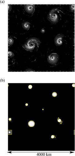
Figure A.1 shows the areas A _{0 ,α} , A _{1 ,α} and A _{2 ,α} that are used to search for the height-dependent rotational centres of 10 TCs at t=8.75 d in the LT RAMS simulation with T _s=30°C and f=10⁻⁴ s⁻¹. In this example, κ=0.5 and β=3.

Fig. A.1.  (a) Reference plot of σ showing N _v=10 significant vortices at t=8.75 d in the LT RAMS simulation with T _s=30°C and f=10⁻⁴ s⁻¹. The greyscale is the same as in Fig. 3. (b) Illustration of the areas used to search for the height-dependent vortex centres. A _0,α covers the white region in the vicinity of a particular vortex; A _1,α covers the white and light grey regions; A _2,α covers the white, light grey and dark grey regions. The boundaries of A _2,α are traced with yellow contours to aid the eye. In general, .

A.3. Note on the horizontal velocity fields used to evaluate asymmetry

Before calculating the radial inflow asymmetry of a TC (δu), the regional mean is subtracted from the horizontal velocity field u ₀ of the boundary layer. The regional mean is here defined as the areal average over a 1000×1000 km² box centred on x _0,α . The magnitude of the regional mean of u ₀ rarely exceeds a few metres per second.

As a final remark, the radius of maximum wind R _n,α (n ∈ {1,2}) appearing in the definition of Tilt (with α dropped) is defined to be the radius that maximises the ϕ-averaged azimuthal component of u _n in a polar coordinate system whose origin is at the TC's rotational centre x _n,α on level n.

References

- Bell M , Montgomery M. T , Emanuel K. E . Air–sea enthalpy and momentum exchange at major hurricane wind speeds observed during CBLAST. J. Atmos. Sci. 2012; 69: 3197–3222.
- Bister M , Emanuel K. A . Dissipative heating and hurricane intensity. Meteorol. Atmos. Phys. 1998; 65: 233–240.
- Black P. G , D'Asaro E. A , French J. R , Drennan W. M , French J. R , co-authors . Air–sea exchange in hurricanes: synthesis of observations from the coupled boundary layer air–sea transfer experiment. Bull. Am. Meteorol. Soc. 2007; 88: 357–374.
- Braun S. A , Tao W.-K . Sensitivity of high-resolution simulations of hurricane Bob (1991) to planetary boundary layer parameterizations. Mon. Weather Rev. 2000; 128: 3941–3961.
- Bryan G . On the computation of pseudoadiabatic entropy and equivalent potential temperature. Mon. Weather Rev. 2008; 136: 5239–5245.
- Bryan G . Effects of surface exchange coefficients and turbulence length scales on the intensity and structure of numerically simulated hurricanes. Mon. Weather Rev. 2012a; 140: 1125–1143.
- Bryan G . Comments on “Sensitivity of tropical-cyclone models to the surface drag coefficient.”. Q. J. Roy. Meteorol. Soc. 2012b
- Bryan G , Rotunno R . The maximum intensity of tropical cyclones in axisymmetric numerical model simulations. Mon. Weather Rev. 2009a; 137: 1770–1789.
- Bryan G , Rotunno R . Evaluation of an analytical model for the maximum intensity of tropical cyclones. J. Atmos. Sci. 2009b; 66: 3042–3060.
- Camargo S. J , Sobel A. H , Barnston A. G , Emanuel K. A . Tropical cyclone genesis potential index in climate models. Tellus A. 2007; 59: 4428–4443.
- Chavas D. R , Emanuel K . Equilibrium tropical cyclone size in an idealized state of a radiative convective equilibrium. 30th Conference on Hurricanes and Tropical. Meteorology, American Meteorology Society. 2012. 10C.4. Online at: https://ams.confex.com/ams/30Hurricane/webprogram/Paper204770.html .
- Cotton W. R , Pielke Sr R. A , Walko R. L , Liston G. E , Tremback C. J , co-authors . RAMS 2001. Current status and future directions. Meterol. Atmos. Phys. 2003; 82: 5–29.
- DeMaria M , Knaff J. A , Schumacher A. B , Kaplan J . Improving tropical cyclone rapid intensity change forecasts. 30th Conference on Hurricanes and Tropical Meteorology. 2012. American Meteorology Society, 8B7. Online at: https://ams.confex.com/ams/30Hurricane/webprogram/Paper204582.html .
- Emanuel K. A . An air sea interaction theory for tropical cyclones. Part I: steady state maintenance. J. Atmos. Sci. 1986; 43: 585–604.
- Emanuel K. A . The maximum intensity of hurricanes. J. Atmos. Sci. 1988; 45: 1143–1155.
- Emanuel K. A . Sensitivity of tropical cyclones to surface exchange coefficients and a revised steady state model incorporating eye dynamics. J. Atmos. Sci. 1995; 52: 3969–3976.
- Emanuel K. A . Tropical cyclone activity downscaled from NOAA-CIRES reanalysis, 1908–1958. J. Adv. Model. Earth Sys. 2010; 2: 1–12.
- Emanuel K. A , Nolan D. S . Tropical cyclone activity and the global climate system. 26th Conference on Hurricanes and Tropical Meteorology. 2004; Miami, FL: American Meteorology Society. 240–241.
- Emanuel K. A , Rotunno R . Self-stratification of tropical cyclone outflow. Part I: implications for storm structure. J. Atmos. Sci. 2011; 68: 2236–2249.
- Frank W. M , Ritchie E. A . Effects of vertical shear on the intensity and structure of numerically simulated hurricanes. Mon. Weather Rev. 2001; 129: 2249–2269.
- Held I. M , Zhao M . Horizontally homogeneous radiative-convective equilibria at GCM resolution. J. Atmos. Sci. 2008; 65: 2003–2013.
- Hill G. E . Factors controlling the size and spacing of cumulus clouds as revealed by numerical experiments. J. Atmos. Sci. 1974; 31: 646–673.
- Jordan C. L . Mean soundings for the West Indies area. J. Meteorol. 1958; 15: 91–97.
- Khairoutdinov M. F , Emanuel K . The effects of aggregated convection in cloud-resolved radiative-convective equilibrium. 30th Conference on Hurricanes and Tropical Meteorology. 2012. American Meteorology Society, 12C.6. Online at: https://ams.confex.com/ams/30Hurricane/webprogram/Paper206201.html .
- Lilly D. K . On the numerical simulation of buoyant convection. Tellus. 1962; XIV: 148–172.
- Lin Y.-L , Farley R. D , Orville H. D . Bulk parameterization of the snow field in a cloud model. J. Clim. Appl. Meteorol. 1983; 22: 1065–1092.
- Louis J. F . A parametric model of vertical eddy fluxes in the atmosphere. Boundary Layer Meteorol. 1979; 17: 187–202.
- Mahrer Y , Pielke R. A . A numerical study of the airflow over irregular terrain. Beitrage zur Physik der Atmosphare. 1977; 50: 98–113.
- Malkus J. S , Riehl H . On the dynamics and energy transformations in a steady-state hurricane. Tellus. 1960; 12: 1–20.
- Montgomery M. T , Bell M. M , Aberson S. D , Black M . Hurricane Isabel (2003). New insights into the physics of intense storms. Part I: mean vortex structure and maximum intensity estimates. Bull. Am. Meteorol. Soc. 2006; 87: 1335–1347.
- Montgomery M. T , Smith R. K , Nguyen S. V . Sensitivity of tropical cyclone models to surface exchange coefficients. Q. J. Roy. Meteorol. Soc. 2010; 136: 1945–1953.
- Ooyama K . Numerical simulation of the life cycle of tropical cyclones. J. Atmos. Sci. 1969; 26: 3–40.
- Ooyama K . Conceptual evolution of theory and modeling of the tropical cyclone. J. Meteorol. Soc. Japan. 1982; 60: 369–379.
- Persing J , Montgomery M. T . Hurricane superintensity. J. Atmos. Sci. 2003; 60: 2349–2371.
- Persing J , Montgomery M. T , McWilliams J. C , Smith R. K . Asymmetric and axisymmetric dynamics of tropical cyclones. Atmos. Chem. Phys. Discuss. 2013; 13: 13323–13438.
- Rappin E. D , Nolan D. S , Emanuel K. A . Thermodynamic control of tropical cyclogenesis in environments of radiative–convective equilibrium with shear. Q. J. Roy. Meteorol. Soc. 2010; 136: 1954–1971.
- Riemer M , Montgomery M. T , Nicholls M. E . A new paradigm for intensity modification of tropical cyclones: thermodynamic impact of vertical wind shear on the inflow layer. Atmos. Chem. Phys. 2010; 10: 3163–3188.
- Riehl H . Some relations between wind and thermal structure of steady state hurricanes. J. Atmos. Sci. 1963; 20: 276–287.
- Rotunno R , Emanuel K. A . An air-sea interaction theory for tropical cyclones: Part II. Evolutionary study using a nonhydrostatic axisymmetric numerical model. J. Atmos. Sci. 1987; 44: 542–561.
- Schecter D. A . Hurricane intensity in the Ooyama (1969) paradigm. Q. J. Roy. Meteorol. Soc. 2010; 136: 1920–1926.
- Schecter D. A . Evaluation of a reduced model for investigating hurricane formation from turbulence. Q. J. Roy. Meteorol. Soc. 2011; 137: 155–178.
- Schecter D. A , Dunkerton T. J . Hurricane formation in diabatic Ekman turbulence. Q. J. Roy. Meteorol. Soc. 2009; 135: 823–838.
- Smagorinsky J . General circulation experiments with the primitive equations. Mon. Weather Rev. 1963; 91: 99–164.
- Smith R. K , Montgomery M. T , Nguyen S. V . Tropical cyclone spin-up revisited. Q. J. Roy. Meteorol. Soc. 2009; 135: 1321–1335.
- Smith R. K , Montgomery M. T , Vogl S . A critique of Emanuel's hurricane model and potential intensity theory. Q. J. Roy. Meteorol. Soc. 2008; 134: 551–561.
- Smith R. K , Thomsen G. L . Dependence of tropical-cyclone intensification on the boundary-layer representation in a numerical model. Q. J. Roy. Meteorol. Soc. 2010; 136: 1671–1685.
- Tang B . Mid-level ventilation's constraint on tropical cyclone intensity. 2010; Massachusetts Institute of Technology, Cambridge, MA, USA,. 195. PhD Dissertation.
- Tang B , Emanuel K . Mid-level ventilation's constraint on tropical cyclone intensity. J. Atmos. Sci. 2010; 67: 1817–1830.
- Tang B , Emanuel K . A ventilation index for tropical cyclones. Bull. Am. Meteorol. Soc. 2012; 93: 1901–1912.
- Velden C , Harper B , Wells F , Beven II J. L , Zehr R , co-authors . The Dvorak tropical cyclone intensity estimation technique. A satellite-based method that has endured for over 30 years. Bull. Am. Meteorol. Soc. 2006; 87: 1195–1210.
- Walko R. L , Band L. E , Baron J , Kittel T. G. F , Lammers R , co-authors . Coupled atmosphere-biophysics-hydrology models for environmental modeling. J. Appl. Meteorol. 2000; 39: 931–944.
- Walko R. L , Cotton W. R , Meyers M. P , Harrington J. Y . New RAMS cloud microphysics parameterization. Part 1: the single-moment scheme. Atmos. Res. 1995; 38: 29–62.
- Yang B , Wang Y , Wang B . The effect of internally generated inner-core asymmetries on tropical cyclone potential intensity. J. Atmos. Sci. 2007; 64: 1165–1188.