A non-hydrostatic global spectral dynamical core using a height-based vertical coordinate

Abstract

Most of the dynamical cores of operational global models can be broadly classified according to the spatial discretisation into two categories: spectral models with mass-based vertical coordinate and grid point models with height-based vertical coordinate. This article describes a new non-hydrostatic dynamical core for a global model that uses the spectral transform method for the horizontal directions and a height-based vertical coordinate. Velocity is expressed in the contravariant basis (instead of the geographical orthonormal basis pointing to the East, North and Zenith directions) so that the expressions of the boundary conditions and the divergence of the velocity are simpler. Prognostic variables in our model are the contravariant components of the velocity, the logarithm of pressure and the logarithm of temperature. Covariant tensor analysis is used to derive the differential operators of the prognostic equations, such as the curl, gradient, divergence and covariant derivative of the contravariant velocity. A Lorenz type grid is used in the vertical direction, with the vertical contravariant velocity staggered with respect to the other prognostic variables. High-order vertical operators are constructed following the finite difference technique. Time stepping is semi-implicit because it allows for long time steps that compensates the cost of the spectral transformations. A set of experiments reported in the literature is implemented so as to confirm the accuracy and efficiency of the new dynamical core.

• dynamical kernel
• Euler equations
• non-hydrostatic
• spectral method
• vertical coordinate

1. Introduction

Spectral transform methods have been widely used in global numerical weather prediction during the last four decades. The first one-level global spectral model was developed by Bourke (1972), including the semi-implicit technique developed by Robert et al. (1972). Soon after, multilevel global models with a spectral horizontal discretisation and a semi-implicit time stepping were developed (e.g. Bourke, 1974; Hoskins and Simmons, 1975; Daley et al., 1976). Global spectral models are characterised by the use of the spherical harmonic functions for the semi-implicit solver and also by the application of the spectral transform method to find the horizontal spatial derivatives of the prognostic variables at the grid points.

Currently, most global spectral models use the set of hydrostatic primitive equations with a hybrid vertical coordinate based on the hydrostatic pressure (Simmons and Burridge, 1981). The Integrated Forecast System (IFS) of the European Centre for Medium-Range Weather Forecasts (ECMWF) (Ritchie et al., 1995) is a reference example with well-known forecasting skills for the medium range (Haiden et al., 2012). A non-hydrostatic extension of the IFS has been recently developed and tested (Wedi and Smolarkiewicz, 2009). The dynamics of this non-hydrostatic version of the IFS follows closely the core of the ALADIN limited-area model formulation (Benard et al., 2010). However, the non-hydrostatic IFS is an exception among the non-hydrostatic global models, since most of them do not use spectral transform methods and have a height-based vertical coordinate [e.g. the UM (Davies et al., 2005) and the NICAM (Satoh et al., 2008)].

The dynamical core presented here is, to the authors’ knowledge, the first non-hydrostatic global spectral model with a height-based vertical coordinate. The height-based coordinate has some pros and cons when compared to the mass-based coordinate. The main disadvantage of height-based coordinate is that it is less stable, as deduced from a linear stability analysis of the one-dimensional vertical acoustic system in an isothermal atmosphere (Bénard, 2003). When considering the three-dimensional set of Euler equations for an unbounded flow, mass-based coordinate is demonstrated to be also more stable than height-based coordinate (Bénard et al., 2004). Height-based coordinate has important advantages in other aspects. One advantage is that it is time independent and, therefore, the metric terms are constant in time: the covariant formulation, also called coordinate-independent formulation, is applied straightforwardly to the Euler equations for time-independent coordinates, but it is much more complicated in the case of time-dependent coordinates (Luo and Bewley, 2004). There are two consequences of using the covariant formulation: the simplification in the formulation of the boundary conditions and the simpler form of the divergence of the velocity. Boundary conditions are as simple as to set the vertical contravariant velocity equal to zero at the upper and lower boundaries, and these conditions can be included in the semi-implicit solver through the definition of the vertical operators, as shown in Section 3. The second advantage of using covariant formulation regards to the divergence: when expressing the divergence as a function of the components of the velocity in the geographical orthonormal basis (pointing East, North and Zenith directions) and using the vertical derivative with respect to a hybrid vertical coordinate, there appears a term that depends on the vertical variation of the horizontal velocity which can lead to numerical problems (Bénard et al., 2005). However, when the contravariant components of the velocity are used, the divergence has a simpler form and this problematic term does not show up. In our model, this simpler expression of the divergence is split in two terms: one is treated implicitly and the other is a pure advection of a metric term related to the difference between the volume densities of the linear and non-linear model geometries, as detailed in Section 2. Another advantage of the height-based coordinate is that it does not require the use of integral operators, unlike the mass-based coordinate. The discrete versions of the differential and integral operators in the ALADIN model must fulfil a set of constraints for solving the semi-implicit linear system (Bubnová et al., 1995), and the finite-difference scheme used in the formulation of the vertical operators is chosen accordingly. With height-based coordinates, there is no need to fulfil constraints for solving the semi-implicit linear system and, therefore, there is more freedom to choose the form and accuracy of the vertical operators.

In summary, from the linear stability point of view, height-based vertical coordinate is worse than mass-based vertical coordinate, and thus a stronger time filter mechanism must be used. On the other hand, height-based vertical coordinate allows an easier implementation of the covariant formulation, which in turn permits a simpler formulation of the boundary conditions and a compact form of the three-dimensional divergence suitable for the semi-implicit technique. Moreover, there are no constraints for the vertical operators to be satisfied in the semi-implicit solver.

This article is divided into the following sections. Section 2 discusses the covariant formulation of the equations, including the linear and non-linear model geometries. The spatial discretisation is described in Section 3. The semi-implicit scheme and the stability analysis are detailed in Section 4. Section 5 describes the results of the tests, and conclusions are summarised in Section 6.

2. Model formulation

In our model, the three-dimensional velocity v, the logarithm of temperature and the logarithm of pressure are the proposed prognostic variables. For this particular set of variables, the system of compressible Euler equations in a reference frame affixed to the Earth is (Zdunkowski and Boot, 2003).1 2 3

where is the angular velocity of the Earth, the geopotential ( being the distance to the centre of the Earth), F the diabatic momentum forcing, Q the diabatic heating rate per unit mass and unit time, the gradient operator, the divergence operator, R the gas constant for dry air, C _p the specific heat capacity of dry air at constant pressure and C _v the specific heat capacity of dry air at constant volume. By using the logarithms of pressure and temperature as prognostic variables, their prognostic equations become linear with respect to the three-dimensional divergence. This is a desirable property as we use the semi-implicit scheme for the time integration where stability is usually enforced when linear and non-linear model equations are similar. The difference between the linear and non-linear prognostic equations is shown in detail in Section 3.

2.1. Covariant formulation

In this work, we explore the use of a fully coordinate-independent formulation of the Euler equations in the context of numerical simulation on the sphere. By ‘coordinate-independent formulation’ we mean that the model equations are written in a curvilinear terrain-following coordinate system, and the velocity, as well as any other tensor, is expressed in the corresponding covariant or contravariant basis of this coordinate system, in contrast to the generalised use of a local orthonormal basis.

The use of a coordinate-independent formulation is not new in numerical weather prediction, e.g. Pielke and Martin (1981), Sharman et al. (1988) and Yang (1993). However, the use of a coordinate-independent formulation for a horizontally spectral fully compressible global model is new.

2.2. Coordinate system

We consider three different coordinate systems in the development of the model equations. First, we consider a Cartesian system referenced to the Earth with coordinates , where the origin is placed at the centre of the Earth, the z axis is in the direction of the north pole, and the x and y axes are in the equatorial plane, with the x axis pointing to the zero longitude meridian. Second, the geographical coordinate system, given by the longitude, latitude and the distance to the centre of the Earth and denoted by . Finally, the model coordinates , which are defined as the geographical longitude and latitude and a hybrid vertical coordinate. The relationship between these coordinates is as follows:4 5 6

and7 8 9

where is a function that depends on the orography. We use the Gal-Chen vertical coordinate Z defined by Gal-Chen and Sommerville (1975):10

where a is the Earth radius, H _T is the height of the rigid top of the spatial domain and represents the orography. Note that the geopotential is simply . An alternative choice for an orography-following vertical coordinate is to use a height-based hybrid coordinate with an exponential vertical decay of the terrain influence (Schär et al., 2002). The entire model formulation is left open to an arbitrary choice of the b function; however, it must satisfy two restrictions: the bottom and top surfaces must be defined by the values Z=0 and Z=1, respectively, and it must ensure that the coordinate transformation is bijective.

2.3. Metric tensor

Following the Riemannian geometry theory (Bär, 2010), a first required step is to derive the metric tensor G in the new coordinates. It can be found from the expression of the metric tensor in Cartesian coordinates, which is the identity, and the Jacobian matrix from Cartesian to model coordinates , by means of the expression . In turn, , where is the Jacobian matrix from Cartesian to geographical coordinates and is the Jacobian matrix from geographical to model coordinates. Thus, is directly derived from eqs. (4)–(6) and can be written as11

Similarly, is found from eqs. (7)–(9) and results12

where b _X , b _Y and b _Z are the partial derivatives of with respect X, Y and Z, respectively. With these results, the metric tensor in the model coordinates is expressed as13

The contravariant metric tensor H is the inverse of the covariant metric tensor. Appendix A.1 shows its components in detail.

Finally, the derivation of the divergence of the velocity, discussed below, requires the expression of the square root of the determinant of the covariant metric tensor, which is

The shallow atmosphere approximation is widely used in global models. It consists in replacing b(X,Y,Z) with the radius of the Earth a in eq. (13). Some of the tests in Section 5 are performed using the shallow atmosphere approximation. The shallow atmosphere metric tensor in model coordinates is14

Observe that horizontal derivatives of are not considered zero in this approximation. From the definition of the vertical coordinate given in eq. (10), it follows that and may not be small, even when the shallow atmosphere approximation is valid.

Still another metric tensor is required for the implementation of the model. The semi-implicit scheme we use for the temporal discretisation involves a linear version of the non-linear eqs. (1)–(3). The linear model must be horizontally homogeneous with constant coefficients in order to efficiently solve the semi-implicit linear system using the spectral transform method. These conditions are fulfilled when the linear model is based on a reference state which is an isothermal and hydrostatically balanced shallow atmosphere at rest with a flat lower boundary. The absence of orography in the linear model is necessary in order to find an exact solution of the linear system at each semi-implicit time step. The linear model geometry is defined by using instead of defined in eq. (9). Note that, despite the linear and non-linear geometries share the same upper boundary and have different lower boundaries, the domain in model coordinates is the same in both geometries (that is, Z ranging from 0 to 1 and X and Y being the longitude and latitude, respectively). The metric tensor for the linear model is found from the shallow atmosphere metric tensor [eq. (14)] substituting with 15

We call the ‘linear metric tensor’ in the sense that it is the metric used for the linear model.

2.4. Free slip boundary conditions

The advantages of using the contravariant velocity as prognostic variable, and specially its vertical component, become clear when applying the free slip conditions at the lower and upper boundaries of the domain, as they are simply at both Z=0 and Z=1. These boundary settings are the same for the linear and non-linear geometries. We cannot emphasize enough the importance of the simplicity of this condition, as no explicit corrections are needed for the vertical velocity obtained at each semi-implicit time step. In the geographical orthonormal basis, the free slip condition at the bottom reads (being w the component of the velocity in the Zenith direction, v the horizontal velocity and the horizontal gradient of the orography). Therefore, w is generally not zero at the lower boundary, and we would not be able to solve the semi-implicit linear system using w, as there is no way to impose the free slip condition for the velocity at the next time step. Nevertheless, w could be used as prognostic variable, although the semi-implicit linear system should be necessarily constructed using W. If w was used as a prognostic variable, its value would be calculated from W and the components of the horizontal velocity. Also, before solving the semi-implicit linear system, the forcing terms for W should have to be calculated from the forcing terms of w and the horizontal velocity. These drawbacks are avoided with the use of the contravariant vertical velocity as prognostic variable.

2.5. Divergence operator

If simple boundary conditions are a strong reason for selecting the contravariant velocity components as prognostic variables, an expression for the divergence of the velocity suitable for the semi-implicit scheme is a second but not less important justification. The divergence is written as16

where are the contravariant components of the velocity and are the model coordinates. Einstein summation over repeated indexes is used (same notation is used throughout the paper when necessary). This form of the divergence is more convenient than the expression found when considering the components of velocity in a locally orthonormal vector basis in the sense that it is more compact. However, the calculation of eq. (16) is computationally expensive, because the horizontal spatial derivatives of must be computed at every time step using the spectral transform method. As the fields computed at each time step are the spectral components of the divergence and vorticity of the horizontal velocity derived with the linear metric tensor (details in Section 4), it is more efficient to express the divergence as17

where is the ‘linear divergence’ in the sense that it is calculated with the ‘linear metric tensor’ . Using eq. (16), it is18

where D is expressed in terms of the horizontal components of the contravariant velocity as follows:19

The second term on the right hand side of eq. (17) involves steady spatial derivatives, which makes its calculation computationally inexpensive, as they can be calculated at the model set up. In fact, it is merely the advection of a constant in time field, and can thus be calculated using both Eulerian or semi-Lagrangian frameworks:

2.6. Gradient operator

The gradient operator applied to any function is

where H is the inverse matrix of G. When working with the linear model, the linear metric tensor is used, and the gradient takes the form

Note that the gradient of the geopotential is very simple. The horizontal components and cancel, whereas the vertical component is20

2.7. Christoffel symbols

Finally, when using the Eulerian advection scheme, the Christoffel symbols are required in order to find the covariant derivative of the contravariant velocity, because

The Christoffel symbols of the Second Kind are given in Appendix A.1.

2.8. Basis change matrices

In this section, we find the basis change matrices between the model contravariant basis and other basis (as the orthonormal basis pointing to the East, North and Zenith directions). The development is presented here for the velocity contravariant vector, but it is equally applicable to any other contravariant tensor. The following notation is used: are the velocity components in the Cartesian coordinates, are the contravariant velocity components in the geographical coordinates, denote the contravariant velocity components in the model coordinates, and are the velocity components in the geographical set of orthonormal vectors pointing to the East, North and Zenith directions. Given the components of the velocity in one basis, they can be changed to any other basis: and ; where and are the Jacobian matrices given in eqs. (11) and (12), respectively. The velocity components in the geographical orthonormal basis, which is the most popular basis when displaying numerical model results, can be calculated from the velocity components in the model basis using , where

2.9. Coriolis term

The full Coriolis inertial term is , and it is applicable in the deep atmosphere case. In the shallow atmosphere approximation, a reduced form of the Coriolis term is used due to energetic consistency concerns (Staniforth and Wood, 2003). Full and reduced versions of the Coriolis inertial term are clearly distinguished when they are written in the geographical orthonormal basis. For a deep atmosphere, the Coriolis term is equal to , where

The Coriolis parameters are and being the angular velocity of the Earth. The matrices and hold the contributions due to f _c and g _c¯ respectively. For the case of the shallow atmosphere approximation, the term is not taken into account (Staniforth and Wood, 2003).

Using the previously described basis change matrices, the Coriolis term can be written in the model coordinate basis as , where ( is the inverse of ). Thus, the Coriolis tensor expressed in the model coordinates is , where21

and22

3. Spatial discretisation

3.1. Horizontal discretisation

In the horizontal dimensions, the prognostic variables are placed onto a Gaussian grid. However, the formulation is open to the use a reduced Gaussian grid (Hortal and Simmons, 1991) with minor changes. This second option is preferable as the number of grid points is smaller, thus reducing the computational cost without significantly reducing the accuracy of the model when the triangular truncation is used. The horizontal fields are transformed between the grid point space to the spherical harmonics space by means of Fourier and Legendre direct and inverse transforms (Bourke, 1972). Derivatives with respect to the horizontal coordinates, denoted with and , are computed in the spectral space. In fact, due to the nature of the spherical harmonic functions, the product is obtained in the spectral space being this magnitude transformed into the grid point space. Finally, the horizontal derivative with respect to latitude is obtained from the grid point value divided by , that is, .

As later described, in order to minimize the number of spectral transformations we follow the method proposed in Temperton (1991) for dealing with the horizontal velocity, its divergence and vorticity.

3.2. Vertical discretisation

The spatial domain is divided in the vertical direction into N layers. These layers are defined by the interfaces between them, the ‘half levels’, plus the lower and upper boundaries (we remark that by definition boundaries are not considered half levels). Half levels and boundaries form a set of N+1 values of the vertical coordinate, from to . The bottom and top boundaries of the domain are defined by and , respectively. Each atmospheric layer is associated with a ‘full level’. Full levels are defined by the set of values of the vertical coordinate, from Z ₁ to Z _N , placed in between half levels (or one of the boundaries and a half level) with values

The distance to the centre of the Earth of the half and full levels depends on the orography and are calculated using the Gal-Chen vertical coordinate given in eq. (10). Therefore, the position of each layer and the interfaces between them is different for each horizontal grid point, but are kept constant in time.

We use the Lorenz vertical grid with all prognostic variables placed at full levels, except the contravariant vertical velocity, which is located over half levels. Note that no unknowns are left at the boundaries since contravariant vertical velocity is zero in both of them.

The model formulation requires two types of vertical operators: the derivative with respect to the vertical coordinate and a vertical interpolation operator. For each of them, two versions are needed: one for functions given at half levels with the result calculated at full levels, and one for the opposite.

As shown in Section 4, the semi-implicit scheme with height-based coordinates do not impose any constraints between operators; therefore, one can freely define the vertical operators and their numerical accuracy.

We derive vertical operators by means of truncated Taylor series around grid points that can, in principle, be chosen to be of any order of accuracy limited ultimately only by the number of levels. Specifically, given P points where a function is known [that is, given to ], a set of equations that allows to estimate the value of the function and its derivatives at the problem point is built:23

From this set of equations, interpolation and derivative are found at the problem point. We observe that higher order derivatives up to P – 1 could also be determined from eq. (23), although, they are not used here.

Altogether, five vertical operators are defined. and are interpolation and derivative operators, which provide results at half levels given the corresponding functions at full levels. They are represented by (N−1)×N matrices. Conversely, and are interpolation and derivative operators, which are applied to functions given at half levels being the results provided at full levels. They are represented by N×(N−1) matrices. The construction of and already assumed that they are applied to functions with zero value at the boundaries (as for the contravariant vertical velocity). Finally, the horizontal momentum prognostic equation requires an interpolator operator from half to full levels over functions that are not zero-valued at the boundaries. This operator is denoted by , and it is represented by a N×(N−1) matrix.

3.3. Non-linear model

In this section, we provide details on the spacial discretisation of the Euler equations in model coordinates. Throughout this and next sections, U, V, r, q represent the set of N values (one for each full level) corresponding to the horizontal components of the contravariant velocity and the logarithm of temperature and pressure, respectively, and W represents the set of N – 1 values (one for each half level) corresponding to the contravariant vertical velocity. These values correspond to a horizontal grid point or to a spectral component, depending on which space they are written. Moreover, and (where g is the gravitational acceleration) denote the values of the geopotential at full and half levels, respectively, obtained from the definition of the vertical coordinate given in eq. (10). On the other hand, metric covariant and contravariant tensors and Christoffel symbols are calculated at full or half levels as needed.

The Euler equations (1)–(3) expressed in model coordinates take the form24 25 26

These equations are not written in conservative form and are not suitable for finite volume methods. The general coordinate formulation is not incompatible with strong conservative methods. A set of equations in strong conservative form for an incompressible flow in general coordinates is discussed in Jørgensen (2003). However, the model described here is based on a spectral solver, and it is not conservative.

Admittedly, a disadvantage of the proposed model is the presence of the Christoffel symbols in the non-linear terms of the momentum equation [eq. (24)], which are not zero in the presence of orography. These terms can lead to instability when the orography is very steep. However, as shown later in Section 5, the model is stable in the presence of steep orography. Moreover, when the semi-Lagrangian scheme is used to solve the advection terms, they can be replaced by upwind interpolations of the momentum components, following the procedure described in Simarro and Hortal (2011).

First, we describe the spatial discretisation of the pressure gradient and gravitational forces in the momentum equation. Taking into account that H ^XY =0, the component is27

This expression is part of the prognostic equation of the contravariant velocity U, and thus is defined at full levels. The first term in eq. (27) is calculated using the horizontal spectral derivative and therefore it is28

where the symbol ‘’ reads ‘discretised as’ and the dot ‘’ means ‘product element by element’. The derivative , as any other derivative of the function b(X,Y,Z), is calculated at each grid point at the model set up stage and read therein during the simulation. The derivative is calculated in the spectral space at the beginning of each time step, and its value at each grid point is found using the inverse spectral transformation.

The second term of eq. (27) is29

The term is treated equally as , and so the resulting discretisation equations are the same [eqs. (28) and (29)] with X substituted by Y. Finally, the component carries on three terms, as none of the H components is zero. The first term is discretised as

and the second is

where is used to interpolate the terms in parentheses to half levels, where the contravariant vertical velocity is defined. Finally, the discretisation of the third term of the pressure and gravitational forces of the contravariant vertical momentum equation writes

As it could be noticed, this discretisation does not use the simple expression for the gradient of the geopotential, which has horizontal components equal zero and vertical component given by eq. (20). Instead, the geopotential gradient is carried along together with the gradient pressure force in all components of the term , the imbalance between pressure gradient and gravitational forces. We have tested several options for the discretisation of this term, and the most stable option was chosen.

Regarding the advection terms in the momentum equation [eq. (1)], these are discretised as follows. The advection terms of the U component of the momentum equation are

plus the following curvature terms:

Similarly, the advection terms of the V component of the momentum equation are discretised as follows:

plus the following curvature terms:

Lastly, the advection terms of the vertical component of the momentum equation are

plus the following curvature terms:

The Coriolis terms are discretised straightforwardly using the matrices [eq. (21) and (22)], and vertical interpolation operators for the velocity components are used where necessary.

In the case of the prognostic equations for the logarithm of temperature [eq. (25)] and the pressure logarithm [eq. (26)], their discretisation is exactly the same, being the only difference a constant. The advection terms are those corresponding to the advection of r itself30

plus the advection31

We remark that the boundary conditions implicitly included in the operator in eqs. (30) and (31) are applied consistently because it operates over a product that includes the vertical contravariant velocity, which is zero at the boundaries.

Finally, taking into account eq. (18), the ‘linear divergence’ term is discretised as follows:32

where D is given in eq. (19). As already mentioned in Section 2, the divergence in eq. (32) is identical to the divergence used in the linear model, called here ‘linear divergence’ because of the use of the ‘linear metric’ .

3.4. Linear model

The linearisation of the Euler equations (24)–(26) is performed assuming a reference state, which consists of an isothermal atmosphere at rest in hydrostatic balance and without orography. This assumption is widely used in spectral models with mass-based vertical coordinates, where the absence of orography is implicit in the assumption of constant hydrostatic pressure at surface (Bénard et al., 2010). The linear model described here is similar to the linear model described in Simarro and Hortal (2011), although with notable differences in the vertical discretisation.

Being the reference temperature, the hydrostatic balance for the reference atmosphere is written as

where is constant and therefore the logarithm of pressure diminishes linearly with the vertical coordinate. Taking into account the linear dependence of the reference logarithm of pressure , the linearisation of the Euler equations (24)–(26) renders

These linear equations are discretised as33 34 35 36 37

This set of linear equations is used in the semi-implicit scheme described in the next section.

4. Semi-implicit scheme and stability

The classical three time level (3TL) semi-implicit scheme is used (Robert, 1981). The numerical instability that comes from the computational mode is damped by using an Asselin time filter (Asselin, 1972). We describe here the Eulerian version, although the extension to a semi-Lagrangian advection is feasible following the procedure in Simarro and Hortal (2011).

The atmospheric state at each time step is represented by a vector function , which contains the values of contravariant velocity, and logarithms of pressure and temperature. The time derivative of at time t _n is approximated by the difference . The forcing terms are replaced by the sum of an explicit non-linear term plus the value of the linear model applied to an average of the values of the atmospheric state at the previous and next time steps, and , respectively. A decentring factor is used to increase the damping of the highest frequency waves. Thus, the 3TL level scheme is represented by the following equation:38

where has been time filtered with the following equation (Asselin, 1972):39

Applying eqs. (33)–(37), the semi-implicit scheme [eqs. (38) and (39)] yields40 41 42 43 44

where and the right hand side terms are explicit values, calculated from known values of the last two time steps. In particular, they include calculated from the spatial discretisation of the Euler equations described in Section 3. A Helmholtz equation can be constructed from this linear system. The procedure is similar to the vertical finite elements (VFEs) version described in Simarro and Hortal (2011). However, some differences appear due to the spherical geometry, mainly in the horizontal components of the momentum equation. In practice, we modify eqs. (40) and (41) to fit the method described in Temperton (1991). To this end, we introduce the definitions , and the following divergence and rotational operators:45 46

Note that is the divergence D given in eq. (19). Taking into account that from eq. (15), the metric terms are and , by applying the operators and to the equations [eq. (40)] and [eq. (41)], we decouple the irrotational and non-divergent components of the horizontal flow:

where the vorticity of the horizontal flow C _n+1 is immediately solved. The other unknowns are related by vertical operators; the Laplacian, being the only horizontal operator, appears applied to the logarithm of pressure.

Therefore, by using eigenfunctions of the horizontal Laplacian, we find a Helmholtz equation for the vertical contravariant velocity, in a similar way proposed by Benard et al. (2010) in the ALADIN model. Once W _n+1 is solved, the other unknowns can be calculated. In order to minimise the number of spectral transformations, the procedure described in Temperton (1991) is followed for the horizontal momentum equation, in particular, for the relations between the divergence and vorticity of the horizontal flow, the horizontal components of the velocity and its horizontal derivatives.

The stability of the 3TL scheme for isothermal and non-isothermal bounded linear atmospheric flows can be studied using a numerical analysis method (Côté, 1983; Bénard et al., 2004). The non-linear model term in eq. (38) is replaced with a linear model , which is exactly the same linear model used in the semi-implicit formulation but with a different reference temperature . Using eqs. (38) and (39) with instead of , the vector states and can be expressed as a function of and , with

being the amplification matrix

where . Eigenvalues of the amplification matrix must have module less or equal to one, otherwise the mode is unstable.

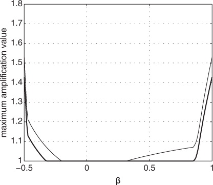
Both the decentring factor ε and the Asselin time filter coefficient α have an impact on the range of stability. Figure 1 (thick line) shows the stability region with and α equal to 0.07 for various wave numbers and residual parameter . The range of stability is wide enough for realistic configurations. In the same figure (thin line), we plotted the same stability test with to show the sensitivity of the range of stability with respect to this parameter.

Fig. 1 Maximum module of the eigenvalues of the amplification matrix for different values of the parameter and wave numbers from 10⁻² m⁻¹ to 10⁻⁶ m⁻¹, using a time step of 1200 s and 40 regularly spaced vertical levels with the top of the atmosphere at 20 km. Asselin time filter coefficient α=0.07. Decentring factor is ε=0 (thin line) and ε=0.07 (thick line).

5. Tests

We describe in this section a set of standard tests in the literature. Both hydrostatic and non-hydrostatic flows are tested, and the results demonstrate the accuracy of the dynamical core.

5.1. Two-dimensional non-hydrostatic flow

A preliminary safety check was performed to the model by coding a two-dimensional slice model with the formulation (and specifically the vertical discretisation) described above. The same tests used by Simarro and Hortal (2011) were also applied to this two-dimensional model, and results were similar (not shown), confirming that the vertical discretisation of the model can simulate non-hydrostatic dynamics accurately. Moreover, the vertical finite difference (VFD) discretisation used here is more robust in presence of steep orography than the VFE scheme reported in Simarro and Hortal (2011).

In our two-dimensional tests, the decentring factor is , the Asselin time filter coefficient and the reference temperature is . We use fourth-order accurate vertical derivative operators and second-order accurate vertical interpolation operators. For non-regular grids, the vertical derivative operator becomes third order, whereas vertical interpolation maintains second-order accuracy. The additional computational cost with respect to second-order vertical derivative operator is smaller than 1%.

The first test we show is the quasi-linear non-hydrostatic test described in Bubnová et al. (1995). It is an idealised test of a two-dimensional flow over a bell-shaped mountain. The flow consists initially of a dry atmosphere with constant stability and horizontal velocity, which is perturbed by the presence of a bell-shaped mountain with maximum height H ₀ and half width a

The setting for this quasi-linear non-hydrostatic wave test is an isothermal atmosphere with Brunt-Väisälä frequency N=0.02 s⁻² and an upstream horizontal velocity of U=15 ms⁻¹. The bell-shaped mountain has H ₀=100 m and a=500 m. The horizontal and vertical resolutions are Δx=100 m and Δz=100 m with the top of the atmosphere placed at H _T =20 km. The absorbing layer begins at 14 km. The integration is done up to with . The results for the vertical velocity are shown in Fig. 2 (left panel) and are very similar to the results in Simarro and Hortal (2011), which is a VFE version of the proposed two-dimensional model. On the other hand, the results given in Fig. 2 are similar to those in Fig. 2 of Bubnová et al. (1995) with respect to the values and positions of the relative maximum and minimum, although there are differences in the details.

Fig. 2 Vertical velocity (contour interval 0.1 ms⁻¹) given by the non-linear model (left) and the linear Boussinesq solution (right) corresponding to the quasi-linear non-hydrostatic flow test. The stability is N=0.02 s⁻¹ and the horizontal initial velocity u =15 ms⁻¹. The mountain parameters are 100 m height and 500 m half width. The results are presented on a domain of 14 km height and 14 km width with the mountain positioned at 3.1 km from the left border of the picture. Horizontal and vertical resolutions are 200 m. Time step is 4 s and the plot corresponds to t=3000 s.

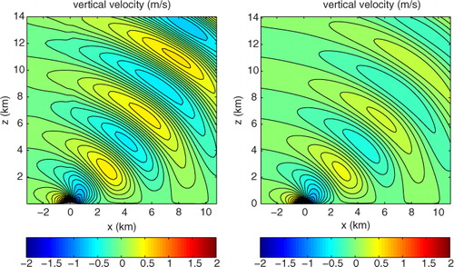
We have included the corresponding steady Boussinesq linear solution (right panel of Fig. 2). It is clear that the non-linear solution given by the model follows closely the Boussinesq solution near the surface. Visible differences appear in the amplitude of the wave above 2 km. It must be taken into account that the Boussinesq approximation makes the assumption of constant density. However, the position and extension of the wave maximums and minimums are similar in both solutions.

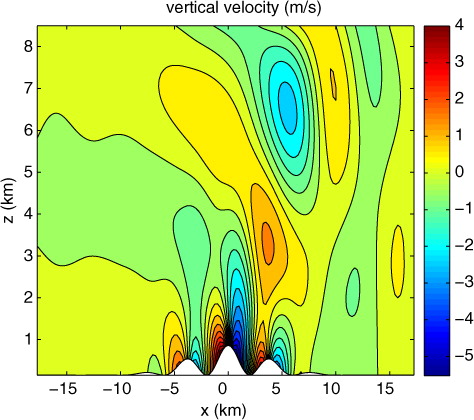
An interesting experiment to test the response of the model with more complex orography is described in (Schär et al., 2002). The upstream profile is defined by a constant value of the Brunt-Väisälä frequency N=0.01 s⁻¹ and the horizontal velocity u=10 ms⁻¹ together with the upstream surface temperature T=288K and pressure p=1000 hPa. The mountain ridge is a bell-shaped structure with superposed small-scale features

where H₀=750 m, a=5000 m and b=4000 m. The gravity waves forced by this mountain have two dominating spectral components: the larger scale is a hydrostatic wave characterised by deep vertical propagation, and the smaller scale is generated by the cosine-shaped terrain variations and is characterised by a rapid decay due to non-hydrostatic effects. The vertical resolution is 150 m, and the horizontal resolution is 250 m. The number of vertical levels is 130. A Rayleigh damping layer is used over a height of 10.7 km to minimise the reflection of vertically propagating waves at the upper boundary. The time step is Δt=4 s. The vertical velocity at time t=40000 s is shown in Fig. 3. The maximum slope for this test is 55%, and the maximum absolute vertical velocity is 5.5 ms⁻¹. Configurations with higher mountains and equal resolution require the use of numerical diffusion in order to prevent numerical instability.

Fig. 3 Vertical velocity at t=1800 s for the Schär test. The time step is Δt=4 s, horizontal resolution Δx=250 m and vertical resolution Δz=150 m. The maximum height of the mountains is 750 m.

Although these two tests are interesting to show how the model performs in the non-hydrostatic regime, they cannot be used to test the convergence of the model to a known analytical solution. In a recently published work, Balfauf and Brdar (2013) found an analytic solution of the compressible Euler equations for linear gravity waves in a channel. We use this known linear analytical solution and compare it with the solution provided by the non-linear model at different configurations.

Balfauf and Brdar considered the evolution of a small initial deviation from a stratified atmosphere which is contained in a two-dimensional channel of a given height and length with periodic boundary conditions. The stratified atmosphere is isothermal, which leads to a constant Brünt-Väisälä frequency and a constant sound speed. Under this assumption, they derive an analytical solution for linear gravity waves by means of a Bretherton transformation (Bretherton, 1966).

We reproduce here the small-scale and non-hydrostatic test reported in Baldauf and Brdar (2013). The initialisation by a warm bubble is a small modification of the gravity wave expansion through a channel proposed by Skamarock and Klemp (1994). The initial warm bubble is

where the temperature perturbation amplitude of the bubble is ΔT=0.01 K, the radius d=5000 m and the position x _c =160 km. The model top is at H=10 km and the channel has a length of L=320 km. The background atmosphere temperature is T ₀=250 K and surface pressure is p _s =1000 hPa. The test is prescribed with an initially constant background flow of u₀=20 m/s. In Fig. 4, we show the linear analytical and the non-linear numerical solutions for the vertical velocity and confirms the good agreement between them in the whole domain. The same test has been repeated with coarser resolutions, maintaining constant the ratio between time step and grid spacing. From results in Table 1, we observe that the numerical solution converges to the analytical solution.

Fig. 4 Vertical velocity at t=1800 s for the Baldauf and Brdar test. The time step is Δt=3.125 s, horizontal resolution Δx=156.25 m and vertical resolution Δz=Δx/2.

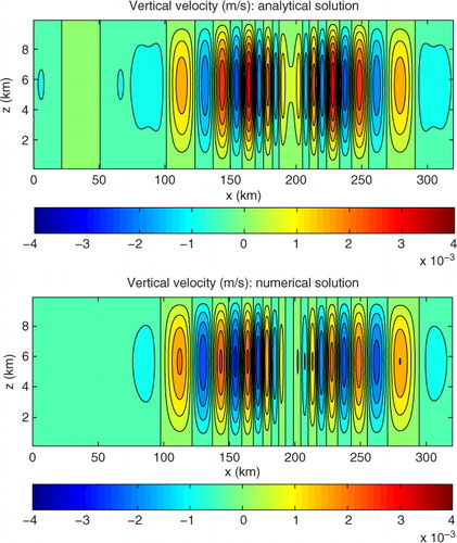
Table 1 Vertical velocity errors for a test configuration with , U=20 ms⁻¹ and . The tests have different horizontal and vertical resolutions and time steps. Vertical resolutions are

Δx (m)	Δt (s)	L 2(×10^5)	L 2(×10^5) L ∞(×10^5)
2500.00	50.000	80.7	370.5
1250.00	25.000	55.8	316.8
625.00	12.500	39.2	222.5
312.50	6.250	31.2	161.2
156.25	3.125	28.0	120.6

There are different sources of error that we want to evaluate. We take account for three of them: the difference between the temperature T ₀ and the reference temperature , whether advection is present or not, and the decentring factor . In particular, we run experiments with all the sources of error present (, u ₀=20 ms⁻¹ and ), without these errors (, and ), and also simulations with each source of error activated independently and sequentially. Results reveal that the decentring factor is the biggest source of error in this case (Table 2).

Table 2 Vertical velocity errors. Tests are configured with different values of the reference temperature, background horizontal velocity and decentring factor. Horizontal resolution is Δx=156.25 m and time step Δt=3.125 s in all cases

	u (ms^−1)		L 2(×10^5)	L ∞(×10^5)
300	20	0.07	28.0	120.6
250	0	0	25.0	78.7
300	0	0	25.6	75.7
250	20	0	25.3	91.4
250	0	0.07	27.4	100.7

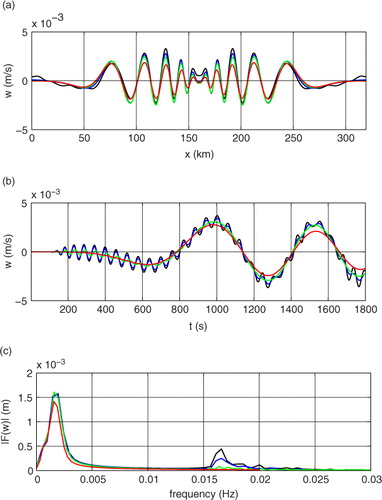
Finally, we compare the linear analytical solution with three numerical solutions (, and ) with different time steps ( equal 12.5 s, 2.5 s and 0.5 s) at the same spatial resolution (Δx=625.0 m and ). Figure 5a shows the vertical velocity of the linear and numerical solutions at z=5000 s and t=1800 s for the whole horizontal domain, whereas Fig. 5b shows the vertical velocity time evolution from the initial state up to t=1800 s at z=5000 m and x=200 km. The convergence towards the linear analytical solution is clear. The frequency spectrum of the vertical velocity at x=200 km and z=5000 m shown in Fig. 5c has two dominating frequencies with periods approximately equal to 500 s and 60 s. The high frequency component of the solution is only reproduced by the test with the smallest time step, whereas the low frequency component is reproduced by all of them being the errors for the larger time step clearly bigger (Fig. 5).

Fig. 5 Vertical velocity of the analytical linear solution (black line) and three numerical tests at the same horizontal resolution (Δx=625.0 m and Δz=Δx/2) and time steps Δt equal 12.5 s, 2.5 s and 0.5 s (red, green and blue lines, respectively). The tests are performed without background horizontal velocity, ε=0.07 and T¯=300K. (a) vertical velocity at t=1800 s and z=5000 m. (b) vertical velocity at x=200 km and z=5000 m. (c) is the frequency spectrum of (b).

In conclusion, these tests reveal that the model can reproduce small-scale non-hydrostatic flows with accuracy, although the semi-implicit scheme for time integration, which is only first order, is a non-negligible source of errors.

5.2. Basic configuration of the three-dimensional tests

The basic model configuration for the tests described in this section is as follows: T42 horizontal resolution, with 64 and 128 grid points in the latitudinal and longitudinal directions, respectively, time step Δt=1200 s, decentring factor , Asselin time filter coefficient , reference temperature , fourth-order accurate vertical derivative operators, second-order accurate vertical interpolation operators and fourth-order linear horizontal diffusion with coefficient 10¹⁶ m⁴ s⁻¹. For the test at T85 horizontal resolution the configuration is the same, except that the number of grid points are 128 and 256, time step is Δt=600 sand the horizontal diffusion coefficient is 10¹⁵ m⁴ s⁻¹. This configuration is similar to the configuration of the Eulerian version of the NCAR CAM3 model in the tests reported in Jablonowski and Williamson (2006) and Lauritzen et al. (2010).

5.3. Three-dimensional Rossby–Haurwitz wave

This test is a three-dimensional extension of the two-dimensional shallow water Rossby–Haurwitz wave (Williamson et al., 1992). The two-dimensional Rossby–Haurwitz wave is an analytical solution of the barotropic vorticity equation, which consists in an unsteady wave that moves westward at a known velocity preserving its shape. The three-dimensional extension is not an analytical solution of the Euler equations, and the shape of the wave is distorted over time. However, during some time, the wave behaves similarly as the two-dimensional case, with a westward translation approximately preserving its shape.

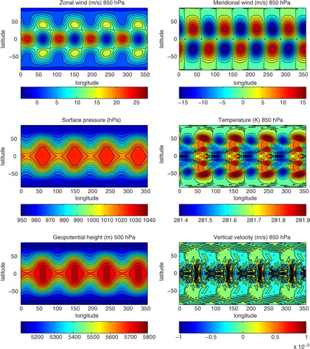
The test has been done at T42 and T85 resolutions with very similar results. Horizontal wind, temperature, geopotential and vertical velocity have been interpolated to the isobaric surfaces of 850 and 500 hPa by cubic spline interpolation. Surface pressure is not directly available and has also been calculated from the logarithm of pressure at full levels by cubic spline interpolation. Results at day 15 for the horizontal wind at 850 hPa, geopotential at 500 hPa and surface pressure (Fig. 6) are very similar to those published in Jablonowski et al. (2008) and Ullrich and Jablonowski (2012). As the flow is almost barotropic, the temperature is almost constant on isobaric surfaces. The 850 hPa temperature forecast for day 15 shown in Fig. 6 (which has a small range of 0.55 K approximately) is very similar to those reported in Jablonowski et al., (2008) and Ullrich and Jablonowski (2012). This is not the case for the vertical velocity, where the hydrostatic result given in Jablonowski et al. (2008) is smoother than those in Ullrich and Jablonowski (2012) and in our model.

Fig. 6 Rossby–Haurwitz wave test at day 15 simulated at T85 with 26 vertical levels. Fields plotted are zonal wind, meridional wind, vertical velocity and temperature at 850 hPa, and surface pressure and geopotential at 500 hPa.

5.4. Steady Jablonowski baroclinic instability rotated test

In the baroclinic instability test developed by Jablonowski and Williamson (2006), the background field is chosen to resemble a realistic state of the real atmosphere. In consequence, this test may indicate whether or not the model is able to reproduce realistic atmospheric motions. The test case is originally formulated in mass-based vertical coordinate. However, it can be translated to height-based vertical coordinates following the procedure described in the appendix of Jablonowski and Williamson (2006). The initial condition is a steady state, adiabatic and frictionless motion in a rotating atmosphere with the shallow approximation. It includes a zonally symmetric basic state with a jet in the mid-latitudes of each hemisphere. The test can be run with or without rotation of the horizontal computational grid.

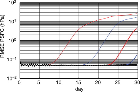
The test has been repeated with three different rotation angles (0°, 45° and 90°) as in Lauritzen et al. (2010) and at two different resolutions (T42 and T85). After some days of integration, due to small truncation errors and the fact that the state is baroclinically unstable, some perturbations begin to grow and the steady state is broken, specially in the rotated cases, where the flow pass over the rotated poles and therefore truncation errors are bigger (Fig. 7). This shows that, although spectral discretisation with triangular truncation has an isotropic accuracy over the sphere, zonal flow direction is privileged over parallel crossing flow directions. The mean square error of the surface pressure (with respect the initial value) is plotted in Fig. 7 for all the experiments. When compared with other models, errors are maintained under 0.5 hPa for longer periods than those of the models reported in Lauritzen et al. (2010), except for the Eulerian version of the spectral hydrostatic CAM model, which shows similar results than the model presented here. As Fig. 7 shows, the error is maintained under 0.5 hPa for more than 30 days for the unrotated case. For 90° rotation angle, the error is maintained under 0.5hPa until days 21 and 30 for T42 and T85 runs, respectively (better results than Eulerian CAM, with errors under 0.5 hPa during the first 20 and 27 d for T42 and T85, respectively). For 45° rotation angle, the error is maintained under 0.5 hPa until day 12 for T42 (while Eulerian CAM cuts the error line of 0.5 hPa at day 19) and day 27 for T85 (equal to Eulerian CAM).

Fig. 7 Jablonowski steady state test. RMSE of surface pressure for rotated angles of 0° (black), 45° (red) and 90° (blue). Bold lines and thin correspond to T85 and T42, respectively.

5.5. Mountain induced Rossby wave train

This test is an adaptation of a similar shallow water test case from Williamson et al. (1992), fully described in Jablonowski et al. (2008). The test is run with mountain heights of 2000 m and 6000 m at resolution T85 and T42, respectively.

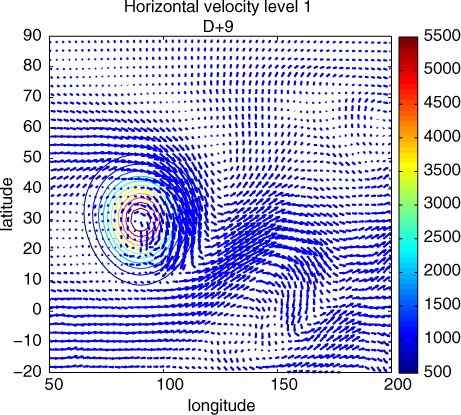
For the 2000 m, height mountain case, geopotential, temperature, zonal and meridional wind at 700 hPa at days 5 and 15 are plotted in Fig. 8. Results at day 5 are very similar to those plotted in Jablonowski et al. (2008), which corresponds to the finite volume version of the CAM model (Lin, 2004). At day 15 results are similar although small differences between both models are visible. For the 6000 m mountain case, topography and horizontal velocity at the first level at day 9 is plotted in Fig. 9.

Fig. 8 Rossby wave train induced by a 2000-m-high mountain at day 5 and 15: geopotential height, zonal and meridional wind at 700 hPa.

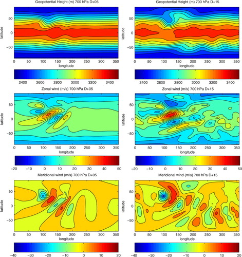
Fig. 9 Rossby wave train induced by a 6000-m-high mountain at day 9. Velocity at level 1 and topography.

5.6. Mass and entropy conservation

Mass and entropy conservation under adiabatic conditions are evaluated. The total mass each time step is calculated as

where is the density at and is the volume around each grid point, estimated with , where for consistency, , and . The following magnitude, related to entropy, must be also conserved

Mass and entropy conservation have been evaluated for all the three-dimensional tests. The results are in Table 3. As expected, identical experiments at different horizontal resolutions tend to produce smaller errors with higher resolution. In the Jablonowski steady test case, error is smaller for the 0° rotation angle, as the steady state is maintained during the 30 d of simulation. However, the error is larger for the 45° and 90° cases (specially for the lower resolution T42) due to the strong baroclinic instability developed during the integration (as shown in Fig. 7). For the 2000 m height mountain case, where metric factors become larger and therefore mass and entropy conservation become more difficult, the model has a relative error of −8.2 10⁻⁶ at day 15 (for both mass and entropy). In the 6000 m height case, the error at day 15 is larger as expected, due both to the lower resolution and the strong instabilities produced in the flow by the mountain. In general, the behaviour is acceptable with respect to mass and entropy conservation.

Table 3 Relative error of total mass and entropy (factor 10⁻⁶) for the different experiments after different integration days

Experiment	Resolution	Day	Mass	Entropy
Rossby–Haurwitz	T42	15	−2.6	−2.7
Rossby–Haurwitz	T85	15	−1.4	−1.4
Mountain 2000	T85	15	−8.2	−8.2
Mountain 6000	T42	15	33.5	33.2
Jablonowski steady state, 0°	T42	30	−2.4	−2.5
Jablonowski steady state, 0°	T85	30	−0.7	−0.7
Jablonowski steady state, 45°	T42	30	−59.8	−60.0
Jablonowski steady state, 45°	T85	30	−2.7	−2.7
Jablonowski steady state, 90°	T42	30	−33.0	−33.3
Jablonowski steady state, 90°	T85	30	−0.7	−0.7

6. Conclusions

A non-hydrostatic dynamical core for a global model has been developed and tested. We use a spectral horizontal discretisation, and the vertical coordinate is based on height and discretised on a Lorenz grid. Vertical operators are derived using the finite difference technique with arbitrary order of accuracy. Standard stability tests revealed a wide range of stable solutions when using a 3TL semi-implicit scheme, although decentring and Asselin time filter coefficients are needed, thus hampering the accuracy of the time stepping. Analytical and non-analytical tests for the model have been implemented, and the model shows notable skill in preserving mass and entropy for long simulation periods. The results of the tests are satisfactory in the sense that the model we have developed possesses high spatial order of accuracy, uses an efficient time integration scheme and shows a wide range of stable solutions.

7. Acknowledgements

G. Simarro would like to express gratitude for the support from the Spanish government through the Ramon y Cajal program.

Appendix

A.1. Contravariant metric and Christoffel symbols

The contravariant metric tensor H is the inverse of the covariant metric tensor given in eq. (13). It is used in the gradient operator, and their components are as follows:

The Christoffel symbols of the Second Kind are used in the advection terms of the momentum equation. They are as follows (Bär, 2010):47

Using metric tensor given in eq. (13), we obtain the following:

In the shallow atmosphere case, is used in eq. (47) instead of G to obtain the Christoffel symbols of the Second Kind . They are written as follows:

References

- Asselin R . Frequency filter for time integrations. Mon. Wea. Rev. 1972; 100: 487–490.
- Baldauf M , Brdar S . An analytic solution for linear gravity waves in a channel as a test for numerical models using the non-hydrostatic. Q.J.R. Meteorol. Soc. 2013
- Bär C . Elementary Differential Geometry. 2010; Cambridge University Press, Cambridge, UK.
- Bénard P . Stability of semi-implicit and iterative centered-implicit time discretizations for various equation systems used in NWP. Mon. Wea. Rev. 2003; 131: 2479–2491.
- Bénard P , Laprise R , Vivoda J , Smolíková P . Stability of leapfrog constant-coefficients semi-implicit schemes for the fully elastic system of Euler equations: flat-terrain case. Mon. Wea. Rev. 2004; 132: 1306–1318.
- Bénard P , Mašek J , Smolíková P . Stability of leapfrog constant-coefficient semi-implicit schemes for the fully elastic system of Euler equations: case with orography. Mon. Wea. Rev. 2005; 133: 1065–1075.
- Bénard P , Vivoda J , Mašek J , Smolíková P , Yessad K , co-authors . Dynamical kernel of the Aladin-NH spectral limited-area model: revised formulation and sensitivity experiments. Q.J.R. Meteorol. Soc. 2010; 136: 155–169.
- Bourke W . An efficient, one-level, primitive-equation spectral model. Mon. Wea. Rev. 1972; 100: 683–689.
- Bourke W . A multi-level spectral model. I. Formulation and hemispheric integrations. Mon. Wea. Rev. 1974; 102: 687–701.
- Bretherton F . The propagation of groups of internal gravity waves in a shear flow. Q.J.R. Meteorol. Soc. 1966; 92: 466–480.
- Bubnová R , Hello G , Bénard P , Geleyn J. F . Integration of the fully elastic equations cast in the hydrostatic pressure terrain-following coordinate in the framework of the ARPEGE/Aladin NWP system. Mon. Wea. Rev. 1995; 123: 515–535.
- Côté J , Beland M , Staniforth A . Stability of vertical discretization schemes for semi-implicit primitive equation models: theory and application. Mon. Wea. Rev. 1983; 111: 1189–1207.
- Daley R , Girard C , Henderson J , Simmonds I . Short-term forecasting with a multi-level spectral primitive equation model. Part I: model formulation. Atmosphere. 1976; 14: 98–116.
- Davies T , Cullen M. J. P , Malcolm A. J , Mawson M. H , Staniforth A , co-authors . A new dynamical core for the Met Office's global and regional modelling of the atmosphere. Q.J.R. Meteorol. Soc. 2005; 133: 1759–1782.
- Gal-Chen T , Sommerville R. C . On the use of a coordinate transformation for the solution of Navier-Stokes. J. Comput. Phys. 1975; 17: 209–228.
- Haiden T , Rodwell M. J , Richardson D. S , Okagaki A , Robinson T , co-authors . Intercomparison of global model precipitation forecast skill in 2010/11 using the SEEPS score. Mon. Wea. Rev. 2012; 140: 2720–2733.
- Hortal M , Simmons A. J . Use of reduced Gaussian grids in spectral models. Mon. Wea. Rev. 1991; 119: 1057–1074.
- Hoskins B. J , Simmons A. J . A multi-layer spectral model and the semi-implicit method. Q.J.R. Meteorol. Soc. 1975; 101: 637–655.
- Jablonowski C , Lauritzen P. H , Taylor M. A , Nair R. D . Idealized test cases for the dynamical cores of atmospheric general circulation models: a proposal for the NCAR ASP 2008 summer colloquium. 2008. http://esse.engin.umich.edu/admg/publications.php .
- Jablonowski C , Williamson D. L . A baroclinic instability test case for atmospheric model dynamical cores. Q.J.R. Meteorol. Soc. 2006; 132: 2943–2975.
- Jørgensen B. H . Tensor formulation of the model equations on strong conservation form for an incompressible flow in general coordinates. 2003. Forskningscenter Risoe. Risoe-R, Denmark. ISBN 87-550-3293-1 (Internet).
- Lauritzen P. H , Jablonowski C , Taylor M. A , Nair R. D . J. Adv. Model. Earth Syst. 2010; 2: 15–34. Rotated versions of the Jablonowski steady-state and baroclinic wave test cases: a dynamical core intercomparison.
- Lin S. J . A vertically Lagrangian finite-volume dynamical core for global models. Mon. Wea. Rev. 2004; 132: 2293–2307.
- Luo H , Bewley T. R . On the contravariant form of the Navier-Stokes equations in time-dependent curvilinear coordinate systems. J. Comput. Phys. 2004; 199: 355–375.
- Pielke R. A , Martin C. L . The derivation of a terrain-following coordinate system for use in a hydrostatic model. J. Atmos. Sci. 1981; 38: 1707–1713.
- Ritchie H , Temperton C , Simmons A , Hortal M , Davies T , co-authors . Implementation of the semi-Lagrangian method in a high-resolution version of the ECMWF forecast model. Mon. Wea. Rev. 1995; 123: 489–514.
- Robert A . A stable numerical integration scheme for the primitive meteorological equations. Atmos. Ocean. 1981; 19: 35–46.
- Robert A , Henderson J , Turnbull C . An implicit time integration scheme for baroclinic models of the atmosphere. Mon. Wea. Rev. 1972; 100: 329–335.
- Satoh M , Matsuno T , Tomita H , Miura H , Nasuno T , co-authors . Nonhydrostatic icosahedral atmospheric model (NICAM) for global cloud resolving simulations. J. Comput. Phys. 2008; 227: 3486–3514.
- Schär C , Leuenberger D , Fuhrer O , Lüthi D , Girard C . A new terrain-following vertical coordinate formulation for atmospheric prediction models. Mon. Wea. Rev. 2002; 130: 2459–2480.
- Sharman R. D , Keller T. L , Wurtele M. G . Incompressible and anelastic flow simulations on numerically generated grids. Mon. Wea. Rev. 1988; 116: 1124–1136.
- Simarro J , Hortal M . A semi-implicit non-hydrostatic dynamical kernel using finite elements in the vertical discretization. Q.J.R. Meteorol. Soc. 2011
- Simmons A. J , Burridge D. M . An energy and angular-momentum conserving vertical finite-difference scheme and hybrid vertical coordinates. Mon. Wea. Rev. 1981; 109: 758–766.
- Skamarock W. C , Klemp J. B . Efficiency and accuracy of the Klemp-Wilhelmson time-splitting scheme. Mon. Wea. Rev. 1994; 122: 2623–2630.
- Staniforth A , Wood N . The deep-atmosphere Euler equations in a generalized vertical coordinate. Mon. Wea. Rev. 2003; 131: 1931–1938.
- Temperton C . On scalar and vector transform methods for global spectral models. Mon. Wea. Rev. 1991; 119: 1303–1307.
- Ullrich P. A , Jablonowski C . MCore: a non-hydrostatic atmospheric dynamical core utilizing high order finite volume methods. J. Comput. Phys. 2012; 231: 5078–5108.
- Wedi N , Smolarkiewicz P. K . A framework for testing global non-hydrostatic models. Q.J.R. Meteorol. Soc. 2009; 135: 469–484.
- Williamson D , Drake J , Hack J , Jakob R , Swarztrauber P . A standard test set for numerical approximations to the shallow water equations in spherical geometry. J. Comput. Phys. 1992; 102: 211–224.
- Yang X . A non-hydrostatic model for simulation of airflow over mesoscale bell-shaped ridges. Boundary-Layer Meteorol. 1993; 65: 401–424.
- Zdunkowski W , Bott A . Dynamics of the Atmosphere: A Course in Theoretical Meteorology. 2003; Cambridge University Press, Cambridge, UK..