Assimilating en-route Lagrangian observations

Abstract

We investigate the assimilation of data that are collected while Lagrangian ocean instruments are in transit between surfacings. We introduce an observation operator that takes these data into account in addition to the data that are typically assimilated. A key point is that the subsurface, en-route paths of these ocean instruments are estimated as part of the assimilation scheme. We present a twin experiment model scenario that lets us compare the improvement by assimilating en-route data over traditional data alone. We make this comparison and present results for both sequential filtering and smoothing.

• data assimilation
• underwater sampling
• Lagrangian instruments
• Eulerian data

1. Introduction

Subsurface observations of the ocean collected in transit by periodically surfacing Lagrangian instruments (ocean gliders and floats) are difficult to use during the assimilation process, and hence are used only in a limited way. We believe this en-route data can be successfully exploited through a modified data assimilation process and inclusion of these data will ultimately prove more efficacious than methods which do not include these data. Over the last decade, there have been marked advances in assimilating novel observations/data types into models. Of specific interest to ocean modelling is the Lagrangian Data Assimilation (LaDA) framework (Ide et al., 2002; Kuznetsov et al., 2003), which incorporates data on a Lagrangian instrument's location into a model of a velocity field. LaDA provides a basis for the strategy that we propose in this article for incorporating subsurface observations of auxiliary quantities (salinity, temperature, pressure, biological quantities) that are typically collected en route. Such data are spatially dependent, but the location where the measurement is taken is unknown since subsurface latitude/longitude measurements are not available. This is the main difficulty in trying to incorporate these data using conventional data assimilation schemes, which require information about the position where measurement is taken. In this article, we propose a form of the observation operator, dictated by the dependence of the measurement location on the Lagrangian path of the instrument, to allow us to assimilate such subsurface data effectively.

The goal of LaDA is to assimilate data collected from Lagrangian instruments – ocean floats and gliders that are advected by the velocity field in which they are taking measurements – into models. Models of such fields are typically defined on grids while observations are not. To overcome this conflict, LaDA methods append equations for the advection of instrument coordinates to the model equations for the velocity field. The resulting observation operator in this methodology is then the identity in the instrument coordinate at observation instances, for example, times at which the instrument has surfaced and where it can report its location. Several theoretical and applied studies have successfully assimilated Lagrangian data in the context of ocean modelling (Salman et al., 2006; Taillandier et al., 2006, 2008; Restrepo, 2008; Salman et al., 2008; Mariano et al., 2011).

Lagrangian instruments can be fitted with a variety of sensors that collect auxiliary subsurface observations (Rudnick et al., 2004; Chyba, 2009; Eriksen and Perry, 2009; Rudnick and Cole, 2011). In the case of Argo floats, subsurface observations are taken both at the parking depth where latitude and longitude are unknown and during ascent where latitude and longitude measurements become available upon surfacing (Gilson and John, 2013; Ollitrault and Rannou, 2013). That is, the measurements of position are available at times when the instrument surfaces while a time series of measurements of the auxiliary variables is available in the intervening period. Similar time series are available for gliders and some of these observations from gliders have been put to limited use in previous studies (Haley et al., 2009; Zhang et al., 2010; Yaremchuk et al., 2011; Jones et al., 2012). Gliders are ‘semi-Lagrangian’ in nature. That is, they can turn and dive by manipulating their buoyancy and rudders as instructed by a pre-programmed flight plan, but their resulting trajectory may be strongly influenced by the local velocity field they are gliding through. Gliders surface frequently (every 6–10 hours) but can surface far from targeted way points. One can foresee that improved assimilation would likely lead to better resolution of local velocity fields which will be beneficial both for assimilating glider data into larger models and for planning future flights. There has been some work on this front (Smith et al., 2010), and we believe fully exploiting data collected en route will help advance glider data assimilation. The scheme that we propose makes full use of such data and additionally aids in the calculation of probability distributions of latitude–longitude–depth paths between surfacing. Such distributions are of particular interest in instances where a glider surfaces far from its predicted surfacing location. Furthermore, the assimilation scheme that we propose also estimates the subsurface path of the Lagrangian instrument. Such assimilated 3-D Lagrangian paths will likely be able to help explore and explain 3-D mixing phenomenon such as the important role that eddies and wind fields play in the meridional overturning conveyor belt theory (Lozier, 2010).

In Section 2, we will review the basics of Lagrangian data assimilation, including the assimilation schemes we use, and also propose an appropriate observation operator for assimilation of subsurface data. To test this methodology, we will perform twin experiments and compare the resulting posterior distributions to those posterior distributions obtained by standard Lagrangian data assimilation. A linearised, shallow water model, which is used as a concrete example for our numerical experiments, is described in Section 3, while the numerical results are presented in Section 4. We end with a few concluding remarks in Section 5.

2. Background and a proposal for assimilation of en-route data

The goal of data assimilation is to incorporate data into physical models to best represent a system of interest, and uncertainty in this representation is typically captured by probability distributions of the representation. This task is often accomplished by utilising the Bayes theorem, . In the assimilation context, we think of and representing the data and state variables of the model, respectively. The goal is then to describe the posterior distribution, , using the likelihood, , and the prior distribution . In the context where the model is time dependent and the data are available as a time series, it is convenient to introduce some shorthand notation and we will use the notation as in Doucet et al. (2001). We will let represent our state variable(s) at time instances and likewise . We will assume that the observations are available at .

To describe the posterior distribution of the state variables for , we need to first do so for the prior distribution and likelihood. Using the assumption that the state variables at different time instances are independent, we can employ the Markov property and the prior distribution becomes where is the prior distribution which reflects uncertainty in initial conditions and is the transition probability. In the case of nonlinear systems/models, transition densities are notoriously difficult to calculate analytically. Similarly, if observation noise is independent, then . Now, we can write down the posterior distribution for a whole sequence of data succinctly. The Bayes theorem in this case gives us:where the marginal distribution in the denominator is given by .

In a typical data assimilation problem, the whole state (e.g. all of the model variables) is not observed. Instead, some subset and/or some function of the model variables are observed. Conventionally, the function that takes model variables to the observation space is called the observation operator. For a given model of the observation noise, the likelihood can (often) be written down explicitly. For simplicity of this discussion, we will assume that the observation noises are normally distributed, independent random variables with covariance Σ. In this case, the likelihood at the j-th observation instance is given by:In the next two subsections, we describe the observation operator for assimilation of Lagrangian data and propose the new observation operator for assimilating subsurface observations whose position is unknown.

2.1. Lagrangian data assimilation

For ocean modelling, typically x or a portion of x describes the fluid flow. We will demarcate these flow variables as x _F . Note that x _F includes all the variables, such as temperature or salinity that are dynamically coupled to the fluid velocity. In the case of Lagrangian data, the drifter position is denoted by x _D . The motion of the Lagrangian drifters is then defined asand of course the drifter's path can be found by integrating this equation. The key to assimilating Lagrangian data is to append the drifter variables to the state space (Ide et al., 2002; Kuznetsov et al., 2003). The extended state space then becomes:and, thus in standard Lagrangian assimilation, the observation operator is simply a projection: . It is worth mentioning at this point that drifter trajectories are often very nonlinear even if the underlying flow model is linear (Apte et al., 2008; Apte and Jones, 2013). This nonlinearity poses great difficulties for assimilation schemes that rely on an assumption of model linearity (Spiller et al., 2008; Apte and Jones, 2013).

2.2. En-route data assimilation

We will now construct the observation operator in the case where the drifter makes measurements of auxiliary quantities, such as salinity or temperature, en route between surfacings, that is, between the times when the position information is available. For concreteness, we will assume measurements of temperature and the state x _F to include the temperature at grid points of a discretised model in 2-D. The measurement of temperature taken by the drifter is of course at the location of the drifter x _D at time t, but this location typically will not be at a grid point. In this case, the temperatures at grid points can be interpolated to the location of the drifter. Suppose x _i for i=1,2,3,4 are the components of x _F denoting the temperature at four points surrounding the drifter location x _D . Then the observation operator we need is written as:where the exact form of the operator h would be determined by the interpolation scheme used, and the last part of the equation only gives the example of linear interpolation in 2-D, with being the weights that sum to unity. Section 3 contains a specific example of the observation operator when the state x _F consists of the Fourier components of the velocity and the auxiliary field (in that case, the height field of linearised, shallow water equations). Note that in both of these cases, the observation operator h is a nonlinear function of the state x.

It should be noted that the subsurface paths themselves are unknown. This means that measurements are being made at locations that are not known. Rather than trying to estimate them in an ad hoc manner, the scheme used here simply treats these locations as unobserved variables. This is possible because of the casting of Lagrangian data assimilation in terms of an augmented system in which the drifter locations are among the state variables. The estimation of the drifter paths then of course happens but as a natural result of the data assimilation scheme.

We would like to note that although the methodology proposed above can be used in any data assimilation scheme, we will focus our demonstrations in Sections 3 and 4 on schemes that have proved successful in the context of Lagrangian data assimilation and its attendant nonlinearity, namely, sequential Monte Carlo or particle filtering and exact sampling method which are explained below.

2.3. Data assimilation schemes

There are a wide variety of data assimilation schemes, all of which share the objective of describing the posterior distribution in some fashion, for example, estimating the mode of the posterior pdf, sampling the posterior pdf or approximations thereof, approximating the posterior pdf as a Gaussian. In this work, we are primarily interested in incorporating novel data in the assimilation process independent of the assimilation scheme utilised. Thus, we will only use two different schemes: sequential Monte Carlo (SMC) or particle filters, and exact posterior sampling. Both of these schemes overcome the difficulty of analytically determining the transition probability densities by sampling them. Thus, these schemes represent the posterior distribution solely on the basis of sampling the components on the right-hand side of Bayes theorem. We will briefly describe these two schemes below, so readers familiar with these methods can move on to Section 3.

Sequential Monte Carlo as typically implemented is a scheme which samples an approximate posterior distribution of interest. Ideally, we seek to sample the posterior distribution as given by the Bayes theorem in eq. (1). In practice, this amounts to generating a number, say N, of samples or ‘particles’ from the prior distribution of the initial conditions . Then, each of these particles are advected according the model evolution until time instance at which point each is compared to y₁, the observation at t ₁, by evaluating the likelihood function . That is, we will now have N samples at t ₁, , k=1,…,N with corresponding probabilities given by:where the likelihood is evaluated, the prior is sampled empirically (e.g. ), and the marginal distribution is estimated with a Monte Carlo integration using the N samples. This process is then repeated sequentially until t=t _j . It is well known that this straightforward sampling strategy breaks down quickly emitting samples with (effectively) zero probability (Doucet et al., 2001).

A commonly used alternative is called the sequential importance resampling (SIR) filter (Liu and Chen, 1998). Importance refers to an importance sampling scheme which replaces the prior distribution at time t _i with the posterior distribution at time t _i−1. In this case, the Bayes theorem becomes:

Algorithmically, this is identical to SMC described above except each sample will have a weight associated with it from the posterior distribution at the previous observation instance instead of the empirical weight (1/N) from sampling the prior distribution directly. Note that there is no change to the locations in state space of the samples generated at any t _i , just a change to their respective weights. Similarly, the expectation used to calculate the marginal distribution is with respect to instead of . Naturally, the exact marginal distribution would be the same in either case. However, approximating the expectation with respect to the posterior from the previous observation time using Monte Carlo is equivalent to approximating the expectation with respect to the prior using importance sampled Monte Carlo. Unfortunately, although this algorithm produces many useful samples, it may also produce many samples with zero weight effectively reducing the sample size of the algorithm. Thus, a technique known as resampling is commonly employed. There are many resampling schemes (van Leeuwen, 2009), but they basically work on the following premise. First, monitor percentage of particles with ‘low’ weights (below some user-set threshold). Once the number of low-weight particles exceeds some user-set acceptable level, replace all particles by empirically sampling the current (t=t _i ) posterior distribution and set all weights to 1/N. Note that this is an application of bootstrapping and often SIR is referred to as a bootstrap filter. This process will effectively cull the low-weight particles and populate regions of state space near high-weight particles. If the model is deterministic, some artificial jitter should be added to the resampled state values to achieve this objective. Then, proceed with sequential importance sampling as before to t=t _i+1 and beyond with continued monitoring of low-weight particles.

2.3.1. Exact sampling.

The above method is a sequential or filtering method since it uses observations at one time instance in one step. In contrast, the exact sampling is a smoothing method in the sense that it uses all data available over a time interval at once, producing the posterior distribution of the initial condition x ₀ conditioned on the observations y _1:j . Thus, the form of the Bayes theorem used in the sampling methods is:where, using the above assumptions of mutual independence of at different time instances and the Markov property for the state,The main idea behind the exact sampling method is to construct a Markov chain whose stationary density is the posterior density for the initial condition x ₀ given in eq. (5). In particular, we use the following Euler–Maruyama discretisation of a Langevin equationas a proposal in a Metropolis–Hastings algorithm, with n=0,1,…,N denoting the steps of the Markov chain. Here, are independent identically distributed (iid) random variables, the proposal covariance Λ is any positive-definite matrix and δ is the step size. The choice of Λ and δ as well as other details of the Metropolis–Hastings algorithm we use are explained in detail in Apte et al. (2008). One of the main issues in the use of this method is the choice of initialisation of this Markov chain. Another one is the often slow convergence of the Markov chain, especially in the case when the nonlinearity is strong. Since our main aim in this article is to propose a framework for assimilating en-route data, we do not discuss these issues here.

3. Illustration of the methodology in a specific example

3.1. Scenario description: linearised, shallow water equation

We will now illustrate the new methodology in a specific context. We will consider the inviscid, linearised, shallow water equations (see Pedlosky, 1986; Apte et al., 2008) as a framework to devise our methodology to include en route, auxiliary data into spectral models for velocity field. These equations are given in a non-dimensional form as:where x, y and t represent spatial dimensions and time, respectively and boundary conditions are taken to be periodic. The scalar velocity components are given by and and the fluid height is represented by . We will approximate the resulting velocity-height field by the zero and first Fourier modes, namely

Note, that the underlying geostrophic mode in eq. (8) is time independent (u ₀ is a constant amplitude) and the first Fourier mode gives a time-varying perturbation to the underlying field with initial conditions . These modes are a solution of eq. (7) if the following dynamics for the time-varying coefficients hold:with initial conditions . Note that in eq. (8), are the solutions of eq. (9) and the value of the velocity-height field perturbations at time t. For simplicity, we will drop the explicit dependence on initial conditions and we will denote the functions on the right-hand side of eq. (9) as . As we are primarily interested in Lagrangian data assimilation, we will also consider tracer motion which is governed by:where the initial glider location is and where are given in eq. (8) [with solutions of the time-varying components in eq. (9)]. Note that the right-hand sides of eq. (10) also depend on . By denoting these functions as and writing these equations together with the drifter equations, our system is governed by:

Note, in this problem scenario is the drifter coordinate and the flow variables x _F =u ₁ the velocity-height field perturbations, , and the full state is .

3.2. Observations

We are considering a scenario where we will know (with relatively large certainty) the position at which the drifter ‘surfaces’ at a given observation instance, , and the objective is to infer the instrument's path between and along with the components of the velocity field. Ultimately, the objective is also to provide a good forecast for for to potentially aid in the choice of control for the next flight path, in the case of gliders. We will denote the time between the ‘surfacing’. Additionally, in between surfacing, the drifter is collecting observations of an auxiliary variable, which is taken to be the height field . We will consider the following two scenarios of assimilation. (1) Only the observations of the drifter locations are assimilated using the LaDA framework. (2) Both the drifter locations and the auxiliary observations are assimilated. As indicated earlier, an obstacle particular to this scenario is that the auxiliary data may be known to relatively high certainty at high frequency, but the spatial locations at which the data are collected are unknown between surfacings, because the instrument's path is unknown.

3.2.1. Lagrangian observations.

In this framework, we will observe the instrument location, periodically in time. Our observations are the ‘true’ location at an observation instant, , plus identical, independently distributed Gaussian random variables which represent observation noise. Thus, the observation operator has the form with where is the observation noise variance (in each direction). (Of course, we could generalise this using any observation noise model.) The resulting likelihood is given in eq. (2) with . Note: such Lagrangian observations have successfully been assimilated by the authors and others in many numerical experiments (Kuznetsov et al., 2003; Salman et al., 2006; Apte et al., 2008; Spiller et al., 2008; Vernieres et al., 2011).

3.2.2. En-route observations.

In addition to the drifter positions, we will observe the height along the unknown instrument path between observation instants. For we will sample the height field with noise, and our observations have the form:13 where is a stationary, zero-mean Gaussian noise process with variance and is the height as given in eq. (8) evaluated along the drifter path , and where is the coefficient of the height mode as determined by eq. (9) for a given . These height observations will be collected at a higher frequency than the surfacing frequency. Suppose that there are K en-route observations of auxiliary variables between surfacing. Thus, we will define en-route observation period given by . Recalling that , the observation operator has the form:14

Note that the motivation for the form of these observations comes from the desire to utilise auxiliary time series of the data that are collected en route, such as salinity measurements. Thus, we are thinking of the fluid height in this simplified model as a proxy for salinity or temperature (or perhaps some other interesting auxiliary data collected by the instrument). The key is that our observation operator depends on an auxiliary variable whose dynamics depends on the flow field and which is sampled along the Lagrangian instrument's path.

3.3. Likelihood

The incorporation of en-route observation shows up in the assimilation process through the observation operator. Specifically, we have two kinds of data – traditional, drifter surfacing locations and a time series of auxiliary data collected between surfacing observations. As the auxiliary data are only available upon surfacing, it will be incorporated into the assimilation scheme at surfacing instances in the case of sequential data assimilation. For the example problem, en-route data collected between will be incorporated along with the location at time . Thus, the observations have the form and the likelihood becomes15 where . In the case of smoothing, the likelihood would be the product of the likelihoods in the form given above and by its very nature, the smoothing method assimilates all the observations at once.

4. Numerical experiments and results

To demonstrate the effect of including data collected between surfacings into the Lagrangian data assimilation process, we will perform twin experiments on the linearised, shallow water model presented in Section 3. That is, we will define the truth to be a run of the simulation with a specific set of initial conditions on and . All assimilations will use data collected at ‘surfacing’, for example, the true drifter path, , sampled periodically in time with observation noise added to those samples. However, the en-route assimilations will also utilise data that are sampled periodically in time (at a higher frequency than surfacings) by evaluating the true height field along the true drifter path, sampling that height at those instances and adding observation noise to those samples.

4.1. Description of experiments

4.1.1. Long-time assimilation: sequential filtering.

For sequential assimilation, we will focus on two sets of initial conditions, both of which lead to strongly nonlinear, Lagrangian drifter paths. The ‘centre’ case has initial conditions given by , and , while the ‘saddle’ case has initial conditions given by and . These cases are both run for where time has been scaled so that the time-varying coefficients [governed by eq. (9)] have a period of one. The drifter paths and height field evaluated along those respective paths for each case are shown in Fig. 1.

Fig. 1 Top: drifter paths for the centre case (left) and the saddle case (right). Note: in both cases a snapshot of the corresponding velocity field is plotted at t=0. Bottom: height field evaluated along drifter paths corresponding to the fields and trajectories shown directly above.

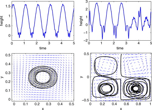
In the study presented here, we seek to compare how well data assimilation can capture the true flow field based on noisy, Lagrangian data. In the twin experiments we perform, the ‘true’ field is determined by the initial conditions of the time-varying coefficients, namely , and in the standard LaDA case, the data are obtained by periodically sampling the true drifter path (as plotted in Fig. 1) and adding observation noise. We will compare results from the standard case to the case where en-route data are also included in the assimilation process. Our proxy for en-route data is the true height field sampled along the true drifter path plus noise. For a fair comparison, in each experiment we will use the same set of drifter observations in both traditional and en-route Lagrangian data assimilation.

We start with broad Normal prior distributions for each of the dimensions with at t=0. Note that the equations for evolution of given by eq. (9) are linear with periodic solutions. Thus, the samples of the prior distribution at t=0 for the flow-field components, will yield the same prior distribution at . In contrast, the evolution of the drifter state is strongly nonlinear, but as the drifter state is observed, we take the variance of the prior distribution to equal the variance of the observation noise. Thus, for we have . We consider a surfacing observations period of and two cases of en-route assimilation with the number of subsurface observations equal to K=9 and .

In all cases, Runge–Kutta simulations use a numerical step size of , precisely , where T is the period of the time-varying coefficients of the flow field.

4.1.2. Short-time assimilation: smoothing.

As mentioned earlier, the exact sampling smoothing method has problems with convergence of the Markov chain used to sample the posterior and these problems are particularly severe for long, highly nonlinear and infrequently observed trajectories. Thus, we use this method only for the case of a short trajectory in the ‘centre’ case and not for the ‘saddle’ case. In particular, the same initial conditions as described above for the centre case are used but the drifter observational period is and the trajectory is for . Another difference is that we sample not only the initial conditions of the velocity variables but also of the drifter positions and the constant amplitude of the geostrophic mode, see eq. (8). [Of course, in this case, we add the equation to eq. (8).] The prior covariance is chosen to be and . The observational noise standard deviation is for the position observations while for the height observations it is and for the ‘low’ and ‘high’ noise cases, respectively. For each of these cases, we consider three different scenarios of an en-route assimilation with the number of subsurface height observations equal to K=9, K=99 and K=999.

4.2. Results

We will consider two measures of the information gained through the assimilation process, both of which characterise the level of certainty in the posterior distribution relative to the prior distribution. First, we will consider the ratio of the determinants of the covariance matrices, , as a function of time (note the superscript a refers to the posterior distribution or analysis while f refers to the prior distribution or forecast). We will also compare the so-called degree of freedom (DOF) for signal, denoted as , which in the case of data assimilation has the form (Zupanski et al., 2007):16 The larger the value of , the more information gained through assimilation and it asymptotes to .

4.2.1. Long-time assimilation: sequential filtering

In the experiments performed here, we are interested in using Lagrangian data and en-route Lagrangian data to find the posterior distribution of the flow field which is governed by .

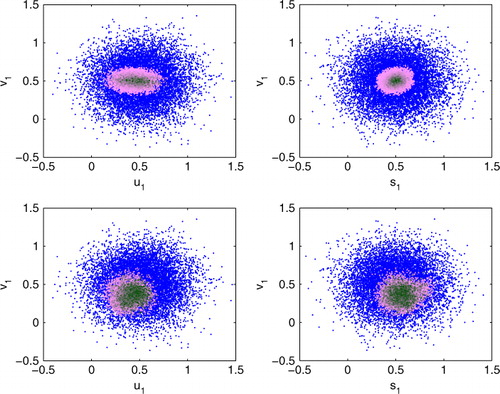
Figure 2 shows projections of samples from the prior distribution and the approximate, discrete posterior distribution for found by assimilating data as described for both standard and en-route cases. Both cases show a near-Gaussian posterior distribution. In the en-route observation case, the posterior distribution is clearly tighter, for example, a posterior distribution with smaller covariance. We also note that the Fourier component s ₁ of the height field (denoted by s ₁ in Fig. 2) is directly coupled to Fourier component v ₁ of the zonal velocity, which in turn is coupled to the Fourier-mode meridional velocity u ₁. Since the auxiliary measurements used in en-route assimilation are that of the height field, the posterior in s ₁ and v ₁ directions is tighter than that in u ₁ direction (lower-left panel in Fig. 2).

Fig. 2 Plotted above are marginal prior and posterior distributions for the saddle case, ‘truth’. Blue dots: projected samples of the prior distribution into the and planes. Pink–black dots: discrete values of posterior distribution, location in plane is state value while colour is weight (pink=0 to black=1). Top: posterior distributions from assimilating standard Lagrangian DA. Bottom: posterior distributions from assimilating en-route observations in addition to standard Lagrangian DA.

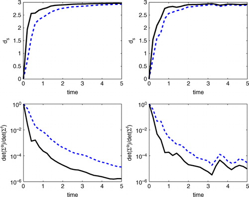
These quantities and were computed for 500 sets of data (same true values for each case with different realisations of observation noise) assimilated for each of the cases defined above. Note that the results for assimilated height observations with K=9 and K=99 are quite similar, so we only show results of the K=9 case when comparing to assimilating standard Lagrangian data assimilation with no height observations. In Fig. 3, the mean over the 500 sets of observations for these two quantities is plotted for both the centre and saddle cases.

Fig. 3 In all figures, solid curves are the mean of assimilating 500 different sets of observations for the same initial condition cases – left column is the centre case, right column is the saddle case. In all cases, solid curves include en-route observations collected along the drifter's path, while dashed lines represent standard Lagrangian data assimilation. Top: ratio of determinants of the posterior distribution to the prior distribution plotted against time. Bottom: as a function of time.

Table 1 includes results for several additional cases. For both the saddle and centre, we consider a ‘high’ en-route observation noise case (where θ is the standard deviation of the position noise in each direction) and a ‘low’ en-route noise case of . In each of these four cases, 500 sets of data were assimilated and averages are taken over those 500 assimilation experiments. In each case, the values of and at t=5 were calculated for each of three combinations of observations depending on the number of en-route observations utilised between each surfacing observation: K=0, K=9 and K=99. It is clear from this table that including en-route data results in tighter posterior distributions and thus more certain estimates. Note that the K=9 and K=99 cases provide roughly the same level of improvement.

Table 1. The averages of and at t=5 and fractions of failure rate for 500 sets of data for the centre and the saddle case, with high and low observational noise levels for using sequential Monte Carlo

Centre (σ s =1.7θ)	Centre (σ s =θ)	Saddle (σ s =1.7θ)	Saddle (σ s =θ)
d a , K=0	2.928	2.926	2.891	2.890
d a , K=9	2.953	2.961	2.908	2.920
d a , K=99	2.954	2.961	2.911	2.921
	1.26×10^−5	1.34×10^−5	2.98×10^−5	2.95×10^−5
	3.46×10^−6	1.70×10^−6	1.82×10^−5	9.77×10^−6
	3.34×10^−6	1.62×10^−6	1.66×10^−5	9.30×10^−6
Posterior err, K=0	0.27	0.26	0.11	0.09
Posterior err, K=9	0.14	0.14	0.04	0.03
Posterior err, K=99	0.15	0.15	0.05	0.03

A potential pit fall of a very tight posterior distribution is that the narrow support of most of the mass may not include the truth. To monitor this, we calculate the fraction of instances over the 500 experiments where the truth fell outside of a 95% confidence interval using the posterior estimate of covariance, at any point during the assimilation, . For both the centre and saddle, even though standard LaDA posterior distributions were not as tight, they had roughly twice the failure rate of identifying the truth. The failure rate over all three cases (K=0, K=9, K=99) is roughly a third smaller for the saddle case, although this may be anticipated as the posterior distributions are not as tight for the saddle case as they are for the centre case. Specific values of these failure rates are listed in the bottom three rows of Table 1.

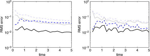
To explore the effects of en-route assimilation versus standard Lagrangian assimilation on the axillary field, we compare the RMS error in each case. Recall, the height field in this example acts as a proxy for a salinity or temperature field. Both assimilation schemes rely on including the drifter coordinates as state variables in addition to the velocity field and the auxiliary field. Coupling between the drifter coordinates and other state variables happens directly through Lagrangian data assimilation setup. That is, in the case of particle-based methods explored here, each particle contains a copy of the full state regardless of which state variables are observed. The dynamics between the observed and unobserved state variables is coupled according to the model equations given in eq. 11. Each particle is propagated forward in time according to these model equations. In a basic sense, evolving a cloud of particles in time according to the dynamic model is the mechanism for sampling prior distributions of the full state. Particles are then weighted (in the case of particle filtering) or kept (in the case of exact filtering) by the considering how ‘close’ the observables of the prior distribution are to observations. The key is that a particle represents the whole state, and for considering the impact of assimilation on the auxiliary field in this example, we can consider the marginal distribution of the Fourier component s ₁ and the fields that correspond to posterior samples of s ₁.

The RMS error of the auxiliary field is calculated by comparing the ‘true’ height field, s, in eq. 8 evaluated at the true value of s ₁(t) to height field evaluated at median valueas found by each assimilation scheme, . Thus we have,Values of this RMS error are plotted in Fig. 4 for both cases considered: centre (left) and saddle (right). These results are the mean of RMS errors calculated by averaging RMS errors found for 500 sets of observations of the same truth. The results for K=9 and K=99 en-route observations between surfacings were nearly identical and the K=99 case was omitted to keep the figure uncluttered. For reference, RMS errors were calculated in the same manner for the 5% of the marginal distribution and are plotted in the same colour/style as the corresponding assimilation scheme, but shaded. (Note: 95% RMS curves were calculated and are quite similar to the 5% curves so they were also omitted for clarity.) In both the centre and saddle cases, one can see that the RMS error of the auxiliary field is smaller for the en-route assimilation than for standard Lagrangian assimilation. Furthermore, the 5% percentiles RMS curves have a general decreasing trend in all cases. Again, those values are lower for the en-route assimilation and notably for the centre case, the 5% RMS error for en-route assimilation is lower than the median RMS error for standard Lagrangian assimilation.

Fig. 4 In both figures, all curves are the mean of RMS error of the height field calculated for 500 different sets of observations for the same initial condition cases – left is the centre case, right is the saddle case. The RMS error compares the difference between the true height field and a ‘median’ height field found through assimilation. In both cases, solid curves correspond to assimilation of en-route observations collected along the drifter's path while dashed lines represent standard Lagrangian data assimilation. For reference, the lightly shaded curves represent RMS error if the 5% percentile height field is compared to the true field.

4.2.2. Short-time assimilation: smoothing.

For the case of smoothing with data from trajectory over a short time, the projection of samples from the prior and the four posteriors (with only Lagrangian data, and with height data with K=9, K=99 and K=999) is shown in the scatterplots in Fig. 5. As expected, we note that with more height observations, the posterior is much tighter. Note the auxiliary variable measured is the height, and from eq. (8), we see that s ₁ is dynamically coupled to v ₁ which in turn is coupled to u ₁, while u ₀ is coupled only to the drifter position x _D . Thus, the posterior in the variables s ₁ and v ₁ shows the most effect of inclusion of height observations. This is clearly reflected in the posterior covariance of each of these variables. Additionally, we see that even though all six variables are uncorrelated in the prior distribution, the posterior shows strong correlations between various variables.

Fig. 5 Plotted above are marginal prior and posterior distributions for the saddle case: , , , is the ‘truth’. In this case, each sample has equal weight and the posterior is simply proportional to the density of samples. Blue dots correspond to the prior, red for pure Lagrangian data, green for K=9 height observations, magenta for K=99, and black for K=999. The bottom-right panel shows the non-convergence rate of the MCMC.

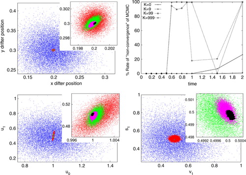
As indicated earlier, the smoothing method suffers from the problem of non-convergence of the MCMC chain used to sample the posterior, in a large part due to the very tight posterior that is obtained with inclusion of all the data at once. Thus, we were not able to run 500 experiments with different noise realisations of the observational noise and find out the ‘failure’ rates as defined above (where a failure is declared to be the case when the truth is outside the 95% confidence interval of the posterior). Instead, we ran the 500 experiments with distinct noise realisations and the bottom-right panel of Fig. 5 shows the percentage of cases when the MCMC failed to converge. This was obtained by running two MCMC instances for each of the 500 cases and when the means of these two instances were outside the 95% confidence interval of the posterior, the case was declared as not converged.

We also see from Fig. 5 that the marginal posterior in the position variables is much tighter when assimilating the height observations (green, magenta and black dots) as compared to the case of not assimilating them. This indicates that the observations of height variable directly affect the estimation of drifter position, because the height field is dynamically coupled to the velocity field, which in turn is coupled to the drifter position.

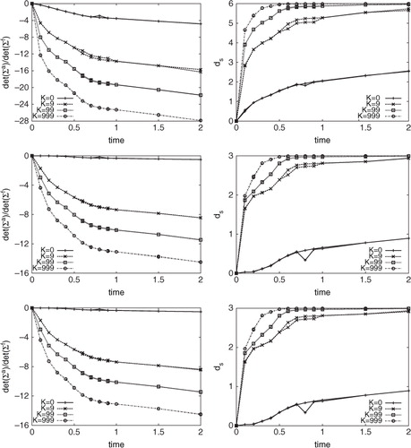
Figure 6 shows the two metrics and as a function of time for this short trajectory case. We see that inclusion of the height observations leads to a faster convergence of towards the asymptotic value (which is equal to the number of degrees of freedom, either three or six, depending on the number of variables we are sampling). Additionally, we can see that the rate of decrease of the ratio of the determinants of the posterior to the prior is more in the case of inclusion of height observations compared with inclusion of only the position observations.

Fig. 6 This figure shows the same metrics as in Fig. 3 as a function of time, but for the case of the short trajectory and using the smoothing method. The top row is for the three variables with low noise in height observations while the middle row is for the three variables with high height observation noise: . The bottom row shows the low noise case but for the posterior on all the six variables: . The two lines for each of the cases correspond to two different realisations of the MCMC chain.

One question that we have not explored in this article is whether the effect of en-route assimilation is only local in space, in the sense that it influences the variables only near the a priori unknown drifter track or whether the effect goes well beyond the vicinity of the drifter track. Since the velocity and height field model we are using is spectral, with only a few Fourier components, our numerical experiments are unable to effectively answer this question and further studies of en-route assimilation with operational ocean models (see, e.g. recent work in Dobricic and Pinardi, 2008; Dobricic et al., 2010; Nilsson et al., 2011, 2012) would certainly be needed.

5. Concluding remarks

We have presented a scheme that enables the assimilation of data collected by Lagrangian ocean instruments while in transit, at depth. Typically, although such data are collected, they have been put to limited use. This is mainly because the data collected at depth (e.g. salinity, temperature, pressure) are challenging to assimilate into spatially dependent models because location information along Lagrangian paths travelled by the instruments is unavailable. To overcome this dilemma, we have introduced an observation operator that takes into account the data collected en route in addition to the data that are typically assimilated. For sequential assimilation, the problem dictates that en-route data only become available at surfacing, and the observation operator is applied at those time instances to assimilate all data collected since the previous surfacing. Of course, in the case of smoothing, both types of data are assimilated together.

We have presented a twin experiment model scenario where we demonstrate the improvement by assimilating en-route data over traditional data alone, both with sequential filtering and smoothing. We use two metrics to compare posterior distribution to prior distributions, and ultimately the amount of information gained through the assimilation process. Additionally, we believe the work presented here is the first step to using en-route data to estimate the unknown Lagrangian paths themselves. In the case of Argo floats which traverse long distances between surfacings, information about the unknown path will prove useful to illuminate the behaviour of Lagrangian trajectories at depth. In the case of gliders which traverse short distances between surfacings, we believe information about semi-Lagrangian path (difference between controlled mission path and the path actually traversed) will prove particularly useful in cases where the glider surfaces far from its destination.

Acknowledgements

This work was supported by the Office of Naval Research, grant number N00014-11-1-0087 and NSF-DMS 1228265.

Notes

¹For simplicity from here forward we will refer to a Lagrangian instrument as the drifter although we are thinking of this methodology as applying to a variety of Lagrangian instruments.

²We use the term novel data in referring to data that are typically collected (e.g. salinity, temperature, and pressure for ocean sampling) but not always used in the assimilation process.

³We would like to emphasise that the main aim of these numerical experiments is to illustrate the efficacy of en-route assimilation scheme proposed above. In particular, we have chosen a simple linear model for the velocity flow and Gaussian prior and observational noise in our identical twin experiments, so as to dissociate these effects from those of en-route data assimilation.

References

- Apte A , Jones C . The effect of nonlinearity on Lagrangian data assimilation. Nonlinear Processes Geophys. 2013; 20: 329–341.
- Apte A , Jones C , Stuart A . A Bayesian approach to Lagrangian data assimilation. Tellus. 2008; 60: 336–347.
- Chyba M . Autonomous underwater vehicles. Ocean Eng. 2009; 36(1): 1.
- Dobricic S , Pinardi N . An oceanographic three-dimensional variational data assimilation scheme. Ocean Model. 2008; 22: 89–105.
- Dobricic S , Pinardi N , Testor P , Send U . Impact of data assimilation of glider observations in the Ionian Sea (Eastern Mediterranean). Dynam. Atmos. Oceans. 2010; 50: 78–92.
- Doucet A , de Freitas N , Gordon N . Sequential Monte Carlo Methods in Practice. 2001; Statistics for Engineering and Information Science, Springer-Verlag, New York..
- Eriksen C , Perry M . The nurturing of seagliders by the national oceanographic partnership program. Oceanography. 2009; 22: 146–157.
- Gilson J . On data collected by Argo floats at parking depth. 2013. Private communication.
- Haley Jr., P. J , Lermusiaux P. F. J , Robinson A. R , Leslie W. G , Logoutov O , co-authors A . Forecasting and reanalysis in the Monterey Bay/California Current region for the Autonomous Ocean Sampling Network-II experiment. Deep Sea Res. Part II – Topical Studies Oceanogr. 2009; 56: 127–148.
- Ide K , Kuznetsov L , Jones C. K. R. T . Lagrangian data assimilation for point vortex systems. J. Turbulence. 2002; 3 Online at: http://www.tandf.co.uk/journals/title/14685248.asp .
- Jones E. M , Oke P. R , Rizwi F , Murray L. M . Assimilation of glider and mooring data into a coastal ocean model. Ocean Model. 2012; 47: 1–13.
- Kuznetsov L , Ide K , Jones C. K. R. T . A method for assimilation of Lagrangian data. Mon. Weather Rev. 2003; 131: 2247–2260.
- Liu J , Chen R . Sequential Monte Carlo methods for dynamic systems. J. Am. Stat. Assoc. 1998; 93: 1032–1044.
- Lozier M . Deconstructing the conveyor belt. Science. 2010; 328: 1507–1511.
- Mariano A , Kourafalou V , Srinivasan A , Kang H , Halliwell G , co-authors . On the modeling of the 2010 Gulf of Mexico oil spill. Dynam. Atmos. Oceans. 2011; 52: 322–340.
- Nilsson A , Dobricic S , Pinardi N , Poulain P.-M , Pettenuzzo D . Variational assimilation of Lagrangian trajectories in the Mediterranean ocean Forecasting System. Ocean Sci. 2012; 8: 249–259.
- Nilsson A , Dobricic S , Pinardi N , Taillandier V , Poulain P.-M . On the assessment of Argo float trajectory assimilation in the Mediterranean Forecasting System. Ocean Dynam. 2011; 61: 1475–1490.
- Ollitrault M , Rannou J.-P . ANDRO: an argo-based deep displacement dataset. J. Atmos. Ocean Tech. 2013; 30: 759–788.
- Pedlosky J . Geophysical Fluid Dynamics. 1986; New York.: Springer.
- Restrepo J . A path integral method for data assimilation. Phys. D. 2008; 237: 14–27.
- Rudnick D , Davis R , Eriksen C , Fratantoni D , Perry M . Underwater gliders for ocean research. Mar. Tech. Soc. J. 2004; 38: 73–84.
- Rudnick D. L , Cole S. T . On sampling the ocean using underwater gliders. J. Geophys. Res. 2011; 116: C08010. DOI: 10.1029/2010JC006849.
- Salman H , Ide K , Jones C. K. R. T . Using flow geometry for drifter deployment in Lagrangian data assimilation. Tellus. 2008; 60: 321–335.
- Salman H , Kuznetsov L , Jones C. K. R. T , Ide K . A method for assimilating Lagrangian data into a shallow-water equation ocean model. Mon. Weather Rev. 2006; 134: 1081–1101.
- Smith R. N , Pereira A , Chao Y , Li P. P , Caron D. A , co-authors . Autonomous underwater vehicle trajectory design coupled with predictive ocean models: a case study. Robotics and Automation (ICRA), 2010 IEEE International Conference on. 2010; IEEE. 4770–4777.
- Spiller E , Budhiraja A , Ide K , Jones C . Modified particle filter methods for assimilating Lagrangian data into a point-vortex model. Phys. D. 2008; 237: 1498–1506.
- Taillandier V , Griffa A , Molcard A . A variational approach for the reconstruction of regional scale Eulerian velocity fields from Lagrangian data. Ocean Model. 2006; 13: 1–24.
- Taillandier V , Griffa A , Poulain P , Signell R , Chiggiato J , co-authors . Variational analysis of drifter positions and model outputs for the reconstruction of surface currents in the central Adriatic during fall 2002. J. Geophys. Res. 2008; 113: C04004.
- van Leeuwen P. J . Particle filtering in geophysical systems. Mon. Weather. Rev. 2009; 137: 4089–4113.
- Vernieres G , Ide K , Jones C. K. R. T . Capturing eddy shedding in the gulf of Mexico from Lagrangian observations. Phys. D. 2011; 240: 166–179.
- Yaremchuk M , Nechaev D , Pan C . A hybrid background error covariance model for assimilating glider data into a coastal ocean model. Mon. Weather. Rev. 2011; 139: 1879–1890.
- Zhang Y , Bellingham J. G , Chao Y . Error analysis and sampling strategy design for using fixed or mobile platforms to estimate ocean flux. J. Atmos. Ocean. Tech. 2010; 27: 481–506.
- Zupanski D , Hou A. Y , Zhang S. Q , Zupanski M , Kummerow D , co-authors . Applications of information theory in ensemble data assimilation. Quart. J. Roy. Meteorol. Soc. 2007; 1545: 1533–1545.