Adaptive ensemble Kalman filtering of non-linear systems

Abstract

A necessary ingredient of an ensemble Kalman filter (EnKF) is covariance inflation, used to control filter divergence and compensate for model error. There is an on-going search for inflation tunings that can be learned adaptively. Early in the development of Kalman filtering, Mehra (1970, 1972) enabled adaptivity in the context of linear dynamics with white noise model errors by showing how to estimate the model error and observation covariances. We propose an adaptive scheme, based on lifting Mehra's idea to the non-linear case, that recovers the model error and observation noise covariances in simple cases, and in more complicated cases, results in a natural additive inflation that improves state estimation. It can be incorporated into non-linear filters such as the extended Kalman filter (EKF), the EnKF and their localised versions. We test the adaptive EnKF on a 40-dimensional Lorenz96 model and show the significant improvements in state estimation that are possible. We also discuss the extent to which such an adaptive filter can compensate for model error, and demonstrate the use of localisation to reduce ensemble sizes for large problems.

• ensemble Kalman filter
• data assimilation
• non-linear dynamics
• covariance inflation
• adaptive filtering

1. Introduction

The Kalman filter is provably optimal for systems where the dynamics and observations are linear with Gaussian noise. If the covariance matrices Q and R of the model error and observation error, respectively, are known, then the standard equations provided originally by Kalman (1960) give the maximum likelihood estimate of the current state. If inexact Q and R are used in Kalman's equations, the filter may still give reasonable state estimates, but it will be suboptimal.

In the case of linear dynamics, Mehra (1970, 1972) showed that the exact Q and R could be reconstructed by auxiliary equations added to the Kalman filter, in the case of Gaussian white noise model error. This advance opened the door for adaptive versions of the filter. More recently, approaches to non-linear filtering such as the extended Kalman filter (EKF) and ensemble Kalman filter (EnKF) have been developed (Evensen, 1994, 2009; Houtekamer and Mitchell, 1998; Kalnay, 2003; Simon, 2006). Proposals have been made (Daley, 1992; Dee, 1995; Anderson, 2007; Li et al., 2009) to extend the idea of adaptive filtering to non-linear filters. However, none of these showed the capability of recovering an arbitrary Q and R simultaneously, even in the simplest non-linear setting of Gaussian white noise model error and observation error. One goal of this article is to introduce an adaptive scheme in the Gaussian white noise setting that is a natural generalisation of Mehra's approach, and that can be implemented on a non-linear Kalman-type filter. We demonstrate the reconstruction of full, randomly generated error covariance matrices Q and R in Example 4.1.

The technique we describe builds on the innovation correlation method of Mehra. Significant modifications are required to lift this technique to the non-linear domain. In particular, we will explicitly address the various stationarity assumptions required by Mehra, which are violated for a non-linear model. As shown by Mehra and later by Daley (1992) and Dee (1995), the innovation correlations are a blended mixture of observation noise, predictability error (due to state uncertainty), and model error. Disentangling them is non-trivial due to the non-stationarity of the local linearisations characteristic of strongly non-linear systems. Many previous techniques have been based on averages of the innovation sequence, but our technique will not directly average the innovations.

Instead, at each filter step, the innovations are used, along with locally linearised dynamics and observations, to recover independent estimates of the matrices Q and R. These estimates are then integrated sequentially using a moving average to update the matrices and used by the filter at time step k. By treating each innovation separately, using the local linearisations relevant to the current state, we are able to recover the full matrices Q and R when the model error is Gaussian white noise, and to improve state estimates in more complicated settings.

Gaussian white noise model error is an unrealistic assumption for practical applications. Typically, more significant model errors, as well as partial observability, must be addressed. In this case, we interpret the covariance matrix [see eq. (2)] as an additive covariance inflation term whose role is to prevent filter divergence and to improve the estimate of the underlying state.

Covariance inflation, originally suggested in the study by Anderson and Anderson (1999), adjusts the forecast error covariance to compensate for systematic underestimation of the covariance estimates given by the Kalman filter. There is a rapidly growing list of approaches to covariance inflation strategies (Desroziers et al., 2005; Constatinescu et al., 2007a, 2007b; Anderson, 2008; Li et al., 2009; Luo and Hoteit, 2011, 2012). In the study by Wang and Bishop (2003), Li et al. (2009) and Hamill et al. (2001), techniques are presented for finding inflation factors that implicitly assume a very simple structure for the noise covariance. There are also many techniques based on the covariance of the implied observation errors at each time step (Mitchell and Houtekamer, 2000; Anderson, 2001; Evensen, 2003; Desroziers et al., 2005; Jiang, 2007). These were actually anticipated and rejected by Mehra (1972), who called them covariance matching techniques. He showed that these techniques were not likely to converge unless the system noise was already known. As untangling the observation noise and system noise is the key difficulty in adaptive filtering, we do not wish to assume prior knowledge of either.

At the same time, new theory is emerging that begins to give mathematical support to particular applications, including the recent article by Gonzalez-Tokman and Hunt (2013) that shows convergence of the EnKF in the sense of the existence of a shadowing trajectory under reasonable hyperbolicity assumptions. In their approach, there is no system noise, and perfect knowledge of the (deterministic) model and the observation noise covariance matrix are necessary to make the proof work. Furthermore, optimality is not addressed, which naturally leads to the question of the optimal choice of the covariance matrices used by the filter. We speculate that an appropriate adaptive filter may be the key to finding the optimal covariance matrices.

We begin the next section by demonstrating the importance of knowing the correct Q and R for the performance of a Kalman filter. Next, we recall the adaptive filter developed in the study by Mehra (1970, 1972) that augments the Kalman filter to estimate Q and R in the case of linear dynamics. In Section 3, we describe an adaptive filter that can find Q and R in real time even for non-linear dynamics and observations, building on the ideas of Mehra. In Section 4, we test the adaptive filter on a 40-dimensional model of Lorenz (1996) and show the dramatic improvements in filtering that are possible. In addition, we show that this adaptive filter can also compensate for significant model error in the Lorenz96 model. We also propose new ideas to extend our technique to the cases of rank-deficient observations and non-additive noise, and discuss an implementation that augments the local ensemble transform Kalman filter (LETKF) version of the EnKF.

2. Extensions of the Kalman filter

Kalman filtering (Kalman, 1960) is a well-established part of the engineering canon for state and uncertainty quantification. In the linear case with Gaussian noise, Kalman's algorithm is optimal. As our main interest is the case of non-linear dynamics, we will use notation that simplifies exposition of two often-cited extensions, EKF and EnKF. For simplicity, we will work in the discrete setting and assume a non-linear model of the following form: 1

where and are zero-mean Gaussian noise with covariance matrices Q and R, respectively. The system is given by f and Q is the covariance of the one-step dynamical noise. The value of an observation is related to x by the function h, with observational noise covariance R. To simplify the notation, we assume the covariance matrices are fixed in time, although in later examples we allow Q and R to drift and show that our adaptive scheme will track slow changes.

We are given a multivariate time series of observations, with the goal of estimating the state x as a function of time. The Kalman filter follows an estimated state and an estimated state covariance matrix . Given the estimates from the previous step, the Kalman update first creates forecast estimates and using the model, and then updates the forecast estimate using the observation . The goal of non-linear Kalman filtering is to correctly interpret and implement the linear Kalman equations 2

where is the covariance of the observation, and is the forecast observation implied by the previous state estimate. The matrices and should be chosen to equal Q and R, respectively, in the linear case; how to choose them in general is the central issue of our investigation. The EKF extends the Kalman filter to systems of the form (1) by explicitly computing linearisations F_k and from the dynamics. In the EnKF, these quantities are computed more indirectly, using ensembles; we give more complete details in Section 4.

Filter performance depends strongly on the covariances and that are used in the algorithm. In fact, for linear problems the algorithm is provably optimal only when the true covariances =Q and =R are used. For non-linear problems, even for Gaussian white noise model error, using the exact =Q can lead to filter instability (see Fig. 5c and d). This is because the local linearisations F_k and introduce an additional model error which may systematically underestimate . More generally, the model error in applications is typically not Gaussian white noise, and must be interpreted as an additive inflation, which attempts to compensate for the covariance structure of the model error.

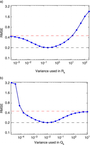
In Fig. 1, we illustrate the effect of various suboptimal and on a non-linear problem by running an EnKF on a 40-site Lorenz96 model (Lorenz, 1996; Lorenz and Emanuel, 1998). (Full details of the model are given in Section 4.) In the limit of large or small , we find that the root mean-squared error (RMSE) of filtered state estimates approach the RMSE of the unfiltered signal. Intuitively, when is large and is small the filter has no confidence in the forecast relative to the observation and the filter simply returns the observation. For a filter to be non-trivial, we must use a smaller and a larger . However, as shown in Fig. 1, when the former is too small or the latter is too large, the RMSE of the filtered signals can actually be higher than the RMSE of the original noisy signals. In one extreme, the filter becomes trivial, and in the other extreme it is possible for the filter to actually degrade the signal. Figure 1 illustrates that a key to filter performance lies in the choice of and .

Fig. 1 Results of EnKF on a Lorenz96 data set (see Section 4) with 400 different combinations of diagonal and matrices. RMSE was computed by comparing the filter output to the time series without observation noise. The correct Q and R (used to generate the simulated data) were diagonal matrices with entries and , respectively. The RMSE of the signal prior to filtering was 0.44 (shown as red dotted line) the RMSE of the optimal filter using and was 0.20 (shown as black dotted line). In (a) we show the effect of varying when and in (b) the effect of varying when .

In Section 3, we present a novel adaptive scheme that augments eq. (2) to also update the matrices and at each filter step based on the observations. As the adaptive scheme is a natural generalisation of the Kalman update, it can be used in many of the extensions of the Kalman filter for non-linear problems.

3. An adaptive non-linear Kalman filter

For the case of linear dynamics with linear full-rank observation, the adaptive filtering problem was solved in two seminal papers (Mehra, 1970, 1972). Mehra considered the innovations of the Kalman filter, which are defined as = and represent the difference between the observation and the forecast. In his innovation correlation method, he showed that the cross-correlations of the innovations could be used to estimate the true matrices Q and R. Intuitively, this is possible because cross-correlations of innovations will be influenced by the system and observation noise in different ways, which give multiple equations involving Q and R. These differences arise because the perturbations of the state caused by the system noise persist and continue to influence the evolution of the system, whereas each observation contains an independent realisation of the observation noise. When enough observations are collected, the resulting system can be solved for the true covariance matrices Q and R.

3.1. Adaptive Kalman filter for linear dynamics

In the case of linear dynamics with linear full-rank observations, the forecast covariance matrix P^f and the Kalman gain K have a constant steady-state solution. Mehra shows that for an optimal filter we have the following relationship between the expectations of the cross-correlations of the innovations and the matrices involved in the Kalman filter:

Now consider the case when the Kalman filter is not optimal, meaning that the filter uses matrices and that are not equal to the true values Q and R. In this case, we must consider the issue of filter convergence. We say that the filter converges if the limit of the state estimate covariance matrices exists and is given by

where is the estimate of the uncertainty in the current state produced by the Kalman filter at time step k. The filter is called non-optimal because the state estimate distribution will have higher variance than the optimal filter, as measured by the trace of M. As shown in the study by Mehra (1970, 1972), for the non-optimal filter, M is still the covariance matrix of the state estimate as long as the above limit exists. Moreover, M satisfies an algebraic Riccati equation given by3

where is the limiting gain of the non-optimal filter defined by and . Note that the matrices Q and R in (3) are the true, unknown covariance matrices.

Motivated by the appearance of the true covariance matrices in the above equations, Mehra gave the following procedure for finding these matrices and hence the optimal filter. After running a non-optimal filter long enough that the expectations in and have converged, the true Q and R can be estimated by solving the following equations: 4

Clearly, this method requires H to be invertible, and when the observation had low rank, Mehra could not recover Q with his method. With a more complicated procedure, he was still able to find the optimal Kalman gain matrix K even when he could not recover Q. However, this procedure used the fact that the optimal gain is constant for a linear model.

3.2. Extension to non-linear dynamics

Our goal is to apply this fundamental idea to non-linear problems. Unfortunately, while the technique of Mehra has the correct basic idea of examining the time correlations of the innovation sequence, there are many assumptions that fail in the non-linear case. First, the innovation sequence is no longer stationary, and thus the expectations for and are no longer well-defined. Second, the matrices H and F (interpreted as local linearisations) are no longer fixed and the limiting values of K and P^f no longer exist, and therefore all of these matrices must be estimated at each filter step. Third, Mehra was able to avoid explicitly finding Q in the case of a rank-deficient observation by using the limiting K, which does not exist in the non-linear case. For non-linear dynamics, the optimal Kalman gain is not fixed, making it more natural to estimate Q directly. When the observations are rank-deficient, parameterisation of the matrix Q will be necessary.

Consequently, the principal issue with lifting Mehra's technique to a non-linear model is that the local linear dynamics are changing with each time step. Even in the case of Gaussian white noise model error, the only quantities that may be assumed fixed over time in the non-linear problem are the covariance matrices Q and R. With this insight, we solve Mehra's equations (4) at each filter step and update and at each step with an exponentially weighted moving average. Thus, our iteration becomes 5

where δ must be chosen small enough to smooth the moving average. Note that these equations naturally augment the Kalman update in that they use the observation to update the noise covariances. This iteration is straightforward to apply with the Extended Kalman Filter, because H_k and F_k are explicitly known. For the EnKF, these quantities must be estimated from the ensembles. This extra step is explained in detail in Section 4.

To explain the motivation behind our method, first consider the following idealised scenario. We assume that the unknown state vector x_k is evolved forward by a known time-varying linear transformation =+ and observed as =+. Furthermore, we assume that and are stationary white noise random variables which are independent of the state, time, and each other, and that =Q and =R. In this scenario, we can express the innovation as

If we were able to average over all the possible realisations of the random variables and (conditioned on all previous observations) at the fixed time k, we would have

However, the most important realisation is that only the last expectation in this equation can be replaced by a time average. This is because unlike , which are independent, identically distributed random variables, the distribution is changing with time and thus each innovation is drawn from a different distribution. In our idealised scenario, the non-stationarity of arises from the fact that the dynamics are time-varying, and more generally for non-linear problems this same effect will occur due to inhomogeneity of the local linearisations.

As we have no way to compute the expectation , we instead compute the matrix

Note that the last two terms have expected value of zero (since =0 for all k), and for each fixed k the difference

has expected value given by the zero matrix. As these terms have expected value of zero for each k, we can now replace the average over realisations of with an average over k since is assumed to be stationary. Thus, we have

where denotes an average over time and denotes an average over possible realisations of the random variable . This motivates our definition of as the empirical estimate of the matrix R based on a single step of the filter. Our method is to first recover the stationary component and then average over time instead of averaging the innovations. Thus, the equation for is simply a moving average of the estimates . Of course, in real applications, the perturbation will not usually be stationary. However, our method is still advantageous since the matrix is largely influenced by and thus by subtracting these matrices we expect to improve the stationarity of the sequence .

A similar argument motivates our choice of and as the empirical estimates of the forecast and model error covariances, respectively. First, we continue the expansion of the k-th innovation as

By eliminating terms which have mean zero, we find the following expression for the cross covariance:

Note that the expected value of is the forecast covariance matrix given by the filter. Solving the above equation for gives an empirical estimate of the forecast covariance from the innovations. This motivates our definition of , the empirical forecast covariance, which we find by solving

It is tempting to use the empirical forecast to adjust the filter forecast ; however, this is infeasible. The empirical forecast is extremely sensitive to the realisation of the noise and since the forecast covariance is not stationary for non-linear problems, there is no way to average these empirical estimates. Instead, we isolate a stationary model error covariance, which can be averaged over time by separating the predictability error from the forecast error.

In our idealised scenario, the forecast error = is the sum of the predictability error and the model error Q that we wish to estimate. We can estimate the predictability error using the dynamics and the analysis covariance from the previous step of the Kalman filter as . Finally, we estimate the model error covariance by

As with , in our example of Gaussian white noise model error, this estimate of is stationary and thus can be averaged over time in order to estimate the true model error covariance Q. While in real applications, the actual form of the forecast error is more complicated, a significant component of the forecast error will often be given by the predictability error estimated by the filter. Thus, it is natural to remove this known non-stationary term before attempting to estimate the stationary component of the model error.

If the true values of Q and R are known to be constant in time, then a cumulative average can be used; however, this would take much longer to converge. The exponentially weighted moving average allows the estimates of and to adjust to slow or sporadic changes in the underlying noise covariances. A large delta will allow fast changes in the estimates but results in and varying significantly. We define = to be the stationarity time scale of our adaptive filter. Any changes in the underlying values of Q and R are assumed to take place on a time scale sufficiently greater than . In the next section, we will show (see Fig. 2) that our iteration can find complicated covariance structures while achieving reductions in RMSE.

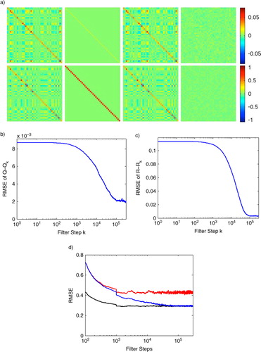
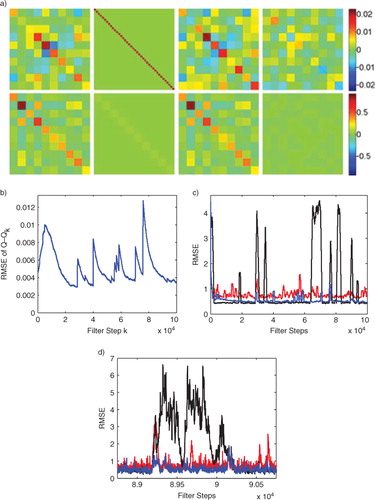
Fig. 2 We show the long-term performance of the adaptive EnKF by simulating Lorenz96 for 300 000 steps and running the adaptive EnKF with stationarity . (a) First row, left to right: true Q matrix used in the Lorenz96 simulation, the initial guess for provided to the adaptive filter, the final estimated by the adaptive filter, and the final matrix difference . The second row shows the corresponding matrices for R; (b) RMSE of as is estimated by the filter; (c) RMSE of as is estimated by the filter; (d) comparison of windowed RMSE vs. number of filter steps for the conventional EnKF run with the true Q and R (black, lower trace), and the conventional EnKF run with the initial guess matrices (red, upper trace), and our adaptive EnKF initialised with the guess matrices (blue, middle trace).

3.3. Compensating for rank-deficient observations

For many problems, H_k or will not be invertible because the number of observations per step m is less than the number of elements n in the state. In this case, the above algorithm cannot hope to reconstruct the entire matrix Q. However, we can still estimate a simplified covariance structure by parameterising = as a linear combination of fixed matrices Q_p . This parameterisation was first suggested by Bélanger (1974). To impose this restriction, we first set

and note that we need to solve =. Thus, we simply need to find the vector q with values q_p that minimise the Frobenius norm

To solve this, we simply vectorise all the matrices involved. Let denote the vector made by concatenating the columns of C_k . We are looking for the least-squares solution of

where the p-th column of A_k is . We can then find the least-squares solution and form the estimated matrix .

In the applications section, we will consider two particular parameterisations of . The first is simply a diagonal parameterisation using n matrices =, where E_ij is the elementary matrix whose only non-zero entry is 1 in the ij position. The second parameterisation is a block-constant structure, which will allow us to solve for in the case of a sparse observation. For the block-constant structure, we choose a number b of blocks which divides n and then we form b ² matrices , where =. Thus, each matrix consists of an × submatrix which is all ones, and they sum to a matrix whose entries are all ones.

Note that it is very important to choose matrices Q_p which complement the observation. For example, if the observations are sparse then the matrix H_k will have rows which are all zero. The block-constant parameterisation naturally interpolates from nearby sites to fill the unobserved entries.

4. Application to the Lorenz model

In this section, we demonstrate the adaptive EnKF by applying it to the Lorenz96 model (Lorenz, 1996; Lorenz and Emanuel, 1998), a non-linear system which is known to have chaotic attractors and thus provides a suitably challenging test-bed. We will show that our method recovers the correct covariance matrices for the observation and system noise. Next, we will address the role of the stationarity parameter and demonstrate how this parameter allows our adaptive EnKF to track changing covariances. Finally, we demonstrate the ability of the adaptive EnKF to compensate for model error by automatically tuning the system noise.

The Lorenz96 model is an N-dimensional ordinary differential equation given by6

where is a vector in and the superscript on xⁱ (considered modulo N) refers to the i-th vector coordinate. The system is chaotic for parameters such as N=40 and F=8, the parameters used in the forthcoming examples. To realise the Lorenz96 model as a system of the form (1), we consider to be the state in at time step k. We define to be the result of integrating the system (6) with initial condition x_k for a single time step of length =. For simplicity, we took the observation function h to be the identity function except in Example 3, where we examine a lower dimensional observation. When simulating the system (1) to generate data for our examples, we generated the noise vector by multiplying a vector of N independent standard normal random numbers by the symmetric positive-definite square root of the system noise covariance matrix Q. Similarly, we generated using the square root of the observation noise covariance matrix R.

In the following examples, we will demonstrate how the proposed adaptive EnKF is able to improve state estimation for the Lorenz96 model. In all of these examples, we will use the RMSE between the estimated state and the true state as a measure of the filter performance. The RMSE will always be calculated over all N=40 observation sites of the Lorenz96 system. In order to show how the error evolves as the filter runs, we will often plot RMSE against filter steps by averaging over a window of 1000 filter steps centred at the indicated filter step. As we are interested in recovering the entire matrices Q and R, we use RMSE to measure the error and . The RMSE in this case refers to the square root of the average of the squared errors over all the entries in the matrices.

The EnKF uses an ensemble of state vectors to represent the current state information. In Examples 4.1–4.4, we will use the unscented version of the EnKF from the study by Julier et al. (2000, 2004). For simplicity, we do not propagate the mean ( in Simon, 2006) or use any scaling. When implementing an EnKF, the ensemble can be integrated forward in time and observed using the non-linear equations (1) without any explicit linearisation. Our augmented Kalman update requires the local linearisations F_k and . While these are assumed available in the extended Kalman filter, for an EnKF these linear transformations must be found indirectly from the ensembles. Let be a matrix containing the ensemble perturbation vectors (the centred ensemble vectors) which represents the prior state estimate and let be the forecast perturbation ensemble which results from applying the non-linear dynamics to the prior ensemble. We define F_k to be the linear transformation that best approximates the transformation from the prior perturbation ensemble to the forecast perturbation ensemble. Similarly, to define we use the inflated forecast perturbation ensemble and the ensemble which results from applying the non-linear observation to forecast ensemble. To summarise, in the context of an EnKF, we define F_k and by 7

where ^† indicates the pseudo-inverse. There are many methods of inflating the forecast perturbation ensemble from . In the examples below, we always use the additive inflation factor by finding the covariance matrix of the forecast ensemble, forming =, and then taking the positive-definite square root of to form the inflated perturbation ensemble .

Example 4.1. Finding the noise covariances

In the first example, both the Q and R matrices were generated randomly (constrained to be symmetric and positive-definite) and the discrete-time Lorenz96 model was simulated for 20000 time steps. We then initialised diagonal matrices and as shown in Fig. 2 and applied the standard EnKF to the simulated data. The windowed RMSE is shown in the red curve of Fig. 2d. Note that the error initially decreases but then quickly stabilises as the forecast covariance given by the EnKF converges to its limiting behaviour.

Next, we applied the adaptive EnKF on the same simulated data using and as our initial guess for the covariance matrices. In Fig. 2a–c, we compare the true Q matrix to the initial diagonal and the final estimate produced by the adaptive EnKF. Here, the adaptive EnKF recovers the complex covariance structure of the system noise in a 40-dimensional system. Moreover, the resulting RMSE, shown by the blue curve in Fig. 2d, shows a considerable improvement. This example shows that for Gaussian white noise model and observation errors, our adaptive scheme can be used with an EnKF to recover a randomly generated covariance structure even for a strongly non-linear model.

Figure 2 shows that the improvement in state estimation builds gradually as the adaptive EnKF converges to the true values of the covariance matrices Q and R. The speed of this convergence is determined by the parameter , which also determines the accuracy of the final estimates of the covariance matrices. The role of the stationarity constant will be explored in the next example.

Example 4.2. Tracking changing noise levels

To demonstrate the role of and to illustrate the automatic nature of the adaptive EnKF, we consider a Lorenz96 system where both Q and R are multiples of the identity matrix, with R being constant and Q varying in time. The trace of Q (normalised by the state dimension N=40) is shown as the black curve in Fig. 3a, where it is compared to the initial Q (shown in red) and the estimates of Q produced by the adaptive EnKF with (shown in green) and (shown in blue). Note that when is smaller the adaptive filter can move more quickly to track the changes of the system; however, when the system stabilises the larger value of is more stable and gives a better approximation of the stable value of Q.

Fig. 3 A Lorenz96 data set with slowly varying Q is produced by defining the system noise covariance matrix Q_k as a multiple of the identity matrix, with the multiple changing in time. (a) Trace of Q_k (black) and for the EnKF (red) compared to the trace of (normalised by N=40) for the Adaptive EnKF at stationarity levels (green) and (blue). (b) Comparison of the RMSE in state estimation for the EnKF with fixed (red) and the Adaptive EnKF with stationarity (green) and (blue). The black curve represents an oracle EnKF which is given the correct covariance matrix Q at each point in time.

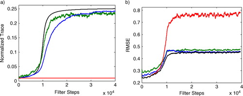
Next, we examine the effect of on the RMSE of the state estimates. Fig. 3b shows that leaving the value of equal to the initial value of Q leads to a large increase in RMSE for the state estimate, while the adaptive EnKF can track the changes in Q. We can naturally compare our adaptive EnKF to an ‘oracle’ EnKF which is given the exact value of Q at each point in time; this is the best case scenario represented by the black curves in Fig. 3. Again, we see that a small results in a smaller peak deviation from the oracle, but the higher stationarity constant tracks the oracle better when the underlying Q is not changing quickly. Thus, the parameter trades adaptivity (lower ) for accuracy in the estimate (higher ).

Example 4.3. Sparse observation

In this example, we examine the effect of a low-dimensional observation on the adaptive EnKF. As explained in Section 3, Mehra uses the stationarity of the Kalman filter for linear problems to build a special adaptive filter for problems with rank-deficient observations. However, our current version of the adaptive EnKF cannot find the full Q matrix when the observation has lower dimensionality than the state vector (possible solutions to this open problem are considered in Section 5). In Section 3, we presented a special algorithm that parameterised the Q matrix as a linear combination of fixed matrices reducing the required dimension of the observation.

To demonstrate this form of the adaptive EnKF, we use a sparse observation. We first observe 20 sites equally spaced among the 40 total sites (below we will consider observing only 10 sites). In this example, the observation y_k is 20-dimensional while the state vector x_k is 40-dimensional, giving a rank-deficient observation. We note that because the observation is sparse the linearisation, H, of the observation will have rows which are all zeros. Solving for requires inverting H so we cannot use the diagonal parameterisation of , and instead we use the block-constant parameterisation which allows the values to be interpolated from nearby sites. In order to check that the adaptive EnKF can still find the correct covariance matrices, we simulated 100000 steps of the discretised Lorenz96 system observing only 20 evenly spaced sites. We take the true Q to have a block-constant structure, and we take the true R to be a randomly generated symmetric positive-definite matrix as shown in Fig. 4. As our algorithm will impose a block-constant structure on , we chose a block-constant matrix for Q so that we could confirm that the correct entry values were recovered.

Fig. 4 We apply the adaptive EnKF with a sparse observation by only observing every other site (20 total observed sites) of a Lorenz96 simulation with 100000 steps. The matrix is assumed to be constant on 4×4 sub-matrices and the true Q used in the simulation is given the same block structure. (a) First row, left to right: true Q matrix used in the Lorenz96 simulation, the initial guess for provided to the adaptive filter, the final estimated by the adaptive filter, and the final matrix difference . The second row shows the corresponding matrices for R; (b) RMSE of as is estimated by the filter; (c) RMSE of as is estimated by the filter; (d) comparison of windowed RMSE vs. number of filter steps for the conventional EnKF run with the true Q and R (black, lower trace), and the conventional EnKF run with the initial guess matrices (red, upper trace), and our adaptive EnKF initialised with the guess matrices (blue, middle trace).

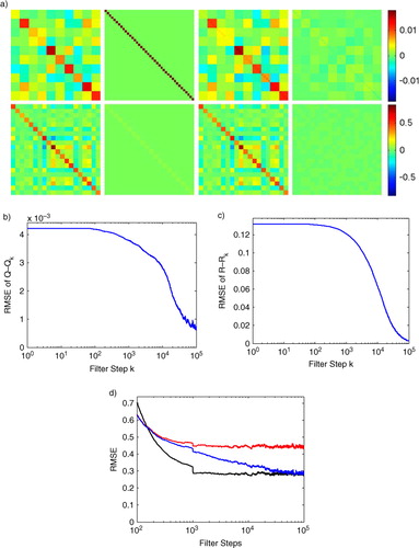
To test the block-constant parameterisation of the adaptive EnKF, we chose initial matrices and which were diagonal with entries 0.02 and 0.05, respectively. We used a large stationarity of _, which requires more steps to converge but gives a better final approximation of Q and R, this is why the Lorenz96 system was run for 100000 steps. Such a large stationarity and long simulation was chosen to illustrate the long-term behaviour of the adaptive EnKF. The estimates of were parameterised with a block-constant structure (b=10 using the method from Section 3). In Fig. 4, we compare the true Q and R matrices to the initial guesses and the final estimates of our adaptive EnKF. This example shows that, even in the case of a rank-deficient observation, the adaptive EnKF can recover an arbitrary observation noise covariance matrix and a parameterised system noise covariance matrix.

Observations in real applications can be very sparse, so we now consider the case when only 10 evenly spaced sites are observed. Such a low-dimensional observation makes state estimation very difficult as shown by the increased RMSE in Fig. 5 compared to Fig. 4. Even more interesting is that we now observe filter divergence, where the state estimate trajectory completely loses track of the true trajectory. Intuitively, this is much more likely when fewer sites are observed, and the effect is shown in Fig. 5c by sporadic periods of very high RMSE. Filter divergence occurs when the variance of is small, implying overconfidence in the state estimate and the resulting forecast. In Fig. 5, this is clearly shown since filter divergence occurs only when the true matrix Q is used in the filter, whereas both the initial guess and the final estimate produced by the adaptive EnKF are inflated. The fact that the filter diverges when provided with the true Q and R matrices illustrates how this example pushes the boundaries of the EnKF. However, our adaptive EnKF produces an inflated version of the true Q matrix as shown in Fig. 5 which not only avoids filter divergence, but also significantly reduces RMSE relative to the initial diagonal guess matrices. This example illustrates that the breakdown of the assumptions of the EnKF (local linearisations, Gaussian distributions) can lead to assimilation error even when the non-linear dynamics is known. In the presence of this error, our adaptive EnKF must be interpreted as an inflation scheme and we judge it by its performance in terms of RMSE rather than recovery of the underlying Q.

Fig. 5 We illustrate the effect of extremely sparse observations by only observing every fourth site (10 total observed sites) of the Lorenz96 simulation, the matrix is assumed to be constant on 4×4 sub-matrices and the true Q used in the simulation is given the same block structure. (a) First row, left to right: true Q matrix used in the Lorenz96 simulation, the initial guess for provided to the adaptive filter, the final estimated by the adaptive filter, and the final matrix difference . The second row shows the corresponding matrices for R; (b) RMSE of as the adaptive EnKF is run; (c) comparison of windowed RMSE vs. number of filter steps for the conventional EnKF run with the true Q and R (black, lower trace), and the conventional EnKF run with the initial guess matrices (red, upper trace), and our adaptive EnKF initialised with the guess matrices (blue, middle trace); (d) Enlarged view showing filter divergence, taken from (c). Note that the conventional EnKF occasionally diverges even when provided the true Q and R matrices. The found by the adaptive filter is automatically inflated relative to the true Q which improves filter stability as shown in (c) and (d).

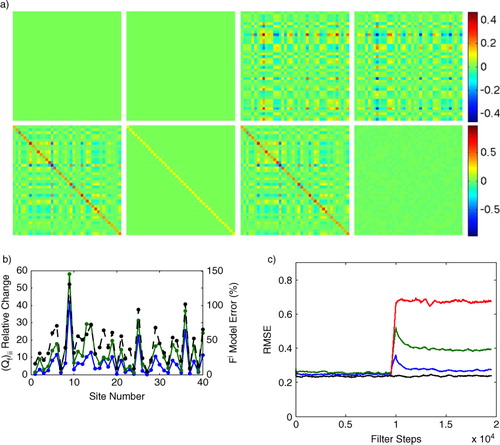
Example 4.4. Compensating for model error

The goal of this example is to show that the covariance of the system noise is a type of additive inflation and thus is a natural place to compensate for model error. Intuitively, increasing increases the gain, effectively placing more confidence in the observation and less on our forecast estimate. Thus, when we are less confident in our model, we would naturally want to increase . Following this line of thought, it seems natural that if is sub-optimally small, the model errors would manifest themselves in poor state estimates and hence large innovations. In this example, the adaptive EnKF automatically inflates based on the observed innovations, leading to significantly improved filter performance.

To illustrate this effect, we fixed the model used by the adaptive EnKF to be the Lorenz96 model from (6) with N=40 and F=8, and changed the system generating the data. The sample trajectory of the Lorenz96 system was created with 20000 time steps. For the first 10000 steps, we set F=8. We then chose N=40 fixed random values of Fⁱ , chosen from a distribution with mean 8 and standard deviation 4. These new values were used for the last 10000 steps of the simulation. Thus, when running our filter we would have the correct model for the first 10000 steps but a significantly incorrect model for the last 10000 steps.

We first ran a conventional EnKF on this data and found that the RMSE for the last 10000 steps was approximately 180% greater than an oracle EnKF which was given the new parameters Fⁱ . Next we ran our adaptive EnKF and found that it automatically increased the variance of in proportion to the amount of model error. In Fig. 6, we show how the variance of was increased by the adaptive filter; note that the increase in variance is highly correlated with the model error measured as the percentage change in the parameter Fⁱ at the corresponding site. Intuitively, a larger error in the Fⁱ parameter would lead to larger innovations thus inflating the corresponding variance in . However, note that when was restricted to be diagonal the adaptive filter required greater increase (shown in Fig. 6b) and gave significantly worse state estimates (as shown in Fig. 6c). Thus, when was not restricted to be diagonal, the adaptive filter was able to find complex new covariance structure introduced by the model error. This shows that the adaptive filter is not simply turning up the noise arbitrarily but is precisely tuning the covariance of the stochastic process to compensate for the model error. This automatic tuning meant that the final RMSE of our adaptive filter increased less than 15% as a result of the model error.

Fig. 6 For the first 10000 filter steps the model is correct and then the underlying parameters are randomly perturbed at each site. The conventional EnKF is run with the initial true covariances and ; the adaptive EnKF starts with the same values but it automatically increases the system noise level () to compensate for the model error resulting in improved RMSE. (a) First row, left to right: true Q matrix used in the Lorenz96 simulation, the initial guess for provided to the adaptive filter, the final estimated by the adaptive filter, and the final matrix difference . The second row shows the corresponding matrices for R; (b) Model error (black, dotted curve) measured as the percent change in the parameter F i at each site compared to the relative change in the corresponding diagonal entries of found with the adaptive EnKF (blue, solid curve), diagonal (green, solid curve). (c) Results of the adaptive EnKF (blue) compared to conventional EnKF (red) on a Lorenz96 data set in the presence of model error. The green curve is an adaptive EnKF, where is forced to be diagonal and the black curve shows the RMSE of an oracle EnKF which is provided with the true underlying parameters F i for both halves of the simulation.

Example 4.5. Adaptive version of the LETKF

The goal of this example is to show that our algorithm can naturally integrate into a localisation scheme. The unscented version of the EnKF used in the previous examples requires large ensemble sizes, which are impractical for many applications. Localisation is a general technique, implemented in various forms, that assumes the state vector has a spatial structure, allowing the Kalman update to be applied locally rather than globally. Some localisation schemes have been shown to allow reduced ensemble size.

The LETKF (Hunt et al., 2004, 2007; Ott et al., 2004) is a localisation technique that is particularly simple to describe. The local update avoids inverting large covariance matrices, and also implies that we only need enough ensemble members to track the local dynamics for each local region. For simplicity, we used the algorithm including the ensemble transform given in eq. (41) of Ott et al. ( 2004). We performed the local Kalman update at each site using a local region with 11 sites (l=5) and we used a global ensemble with 22 members, compared to 80 ensemble members used in the unscented EnKF.

Building an adaptive version of the LETKF is fairly straightforward. A conventional Kalman update is used to form the local analysis state and covariance estimates. We design an adaptive LETKF by simply applying our iteration, given by eq. (5), after the local Kalman update performed in each local region. We will estimate 40 separate pairs of matrices and . This implies that some entries in the full (those far from the diagonal) have no representatives in these local . Moreover, the other entries in the full are represented by entries in several matrices. In Fig. 7, we combine the final estimates of into a single matrix by averaging all the representatives of each entry. It would also be possible to form this global matrix at each step; however, the LETKF often allows many choices for forming the global results from the local, and our objective here is only to show that our adaptive iteration can be integrated into a localised data assimilation method.

Fig. 7 We compare the conventional and adaptive LETKF on a simulation of 300000 steps of Lorenz96 (a) First row, left to right: benchmark matrix where Q is was the matrix used in the Lorenz96 simulation, the initial guess for provided to the adaptive filter, the final estimated by the adaptive filter, and the final matrix difference . The second row shows the corresponding matrices for R (leftmost is the true R); (b) the variances from the diagonal entries of the true Q matrix (black, rescaled to range from 0 to 1) and the those from the final global estimate produced by the adaptive LETKF (blue, rescaled to range from 0 to 1) (c) Results of the adaptive LETKF (blue) compared to conventional LETKF with the diagonal covariance matrices (red) and the conventional LETKF with the benchmark covariances = and (black).

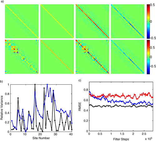
Interestingly, the conventional LETKF requires significant inflation to prevent filter divergence. For example, the noise variances in Fig. 7 are comparable to Example 4.1; however, the LETKF often diverges when the diagonal entries of are less than 0.05. So, for this example we use = and as the benchmark for all comparisons, since this represents a filter which was reasonably well-tuned when the true Q and R were both known. To represent that case when the true Q and R are unknown, we choose diagonal matrices with the same average covariance as and R, respectively. For the conventional LETKF, we form the local and by simply taking the sub-matrices of and which are given by the local indices. In Fig. 7, we show that the adaptive LETKF significantly inflates both and , and it recovers much of the structure of both Q and R, and improves the RMSE, compared to the conventional LETKF using the diagonal and .

While this example shows that our iteration can be used to make an adaptive LETKF, we found that the adaptive version required a much higher stationarity ( in Fig. 7). We speculate that this is because local regions can experience specific types of dynamics for extended periods which bias the short-term estimates and by setting a large stationarity we remove these biases by averaging over a larger portion of state space. We also found that the LETKF could have large deviations from the true state estimate similar to filter divergence but on shorter time scales. These deviations would cause large changes in the local estimates which required us to impose a limit of on the amount an entry of could change in a single time step of 0.05. It is possible that a better tuned LETKF or an example with lower noise covariances would not require these ad hoc adjustments. As large inflations are necessary simply to prevent divergence, this adaptive version is a first step towards the important goal of optimising the inflation.

5. Discussion and outlook

A central feature of the Kalman filter is that the innovations derived from observations are only used to update the mean state estimate, and the covariance update does not incorporate the innovation. This is a remnant of the Kalman filter's linear heritage, in which observation, forecast and analysis are all assumed Gaussian. In any such scenario, when a Gaussian observation is assimilated into a Gaussian prior, the posterior is Gaussian and independent of observation. Equation (2) explicitly shows that the Kalman update of the covariance matrix is independent of the innovation.

Any scheme for adapting the Kalman filter to non-linear dynamics must consider the possibility of non-Gaussian estimates, which in turn demands a re-examination of this independence. However, the stochastic nature of the innovation implies that any attempt to use this information directly will be extremely sensitive to particular noise realisations. In this article, we have introduced an augmented Kalman update in which the innovation is allowed to affect the covariance estimate indirectly, through the filter's estimate of the system noise. We envision this augmented version to be applicable to any non-linear generalisation of the Kalman filter, such as the EKF and EnKF. Application to the EKF is straightforward, and we have shown in eq. (7) how to implement the augmented equations into an ensemble Kalman update.

The resulting adaptive EnKF is an augmentation of the conventional EnKF, to allow the system and observation noise covariance matrices to be automatically estimated. This removes an important practical constraint on filtering for non-linear problems, since often the true noise covariance matrices are not known a priori. Using incorrect covariance matrices will lead to sub-optimal filter performance, as shown in Section 2, and in extreme cases can even lead to filter divergence. The adaptive EnKF uses the innovation sequence produced by the conventional equations, augmented by our additional equations developed in Section 3, to estimate the noise covariances sequentially. Thus, it is easy to adopt for existing implementations, and as shown in Section 4 it has a significant performance advantage over the conventional version. Moreover, we have shown in Section 4 that the adaptive EnKF can adjust to non-stationary noise covariances and even compensate for significant modelling errors.

The adaptive EnKF introduced here raises several practical and theoretical questions. A practical limitation of our current implementation is the requirement that the rank of the linearised observation H_k is at least the dimension of the state vector x_k . In Section 3, we provide a partial solution which constrains the Q estimation to have a reduced form which must be specified in advance. However, in the context of the theory of embedology, developed in the study by Sauer et al. (1991), it may be possible to modify our algorithm to recover the full Q matrix from a low-rank observation. Embedology shows that for a generic observation, it is possible to reconstruct the state space using a time-delay embedding. Motivated by this theoretical result, we propose a way to integrate a time-delay reconstruction into the context of a Kalman filter and discuss the remaining challenges of such an approach.

In order to recover the full system noise covariance matrix in the case of rank-deficient observation, we propose an augmented observation formed by concatenating several iterations of the dynamics,

which will be compared to time-delayed observation vector = For a generic observation h, when the system is near an attractor of box counting dimension N, our augmented observation is generically invertible for (Sauer et al., 1991). We believe that this augmented observation will not only solve the rank-deficient observation problem, but may also improve the stability of the Kalman filter by including more observed information in each Kalman update. However, a challenging consequence of this technique is that the augmented observation is influenced by both the dynamical noise and the observation noise realisations. Thus extracting the noise covariances from the resulting innovations may be non-trivial.

An important remaining theoretical question is to develop proofs that our estimated Q and R converge to the correct values. For R this is a straightforward claim, however the interpretation of Q for non-linear dynamics is more complex. This is because the Kalman update equations assume that at each step the forecast error distribution is Gaussian. Even if the initial prior is assumed to be Gaussian, the non-linear dynamics will generally change the distribution, making this assumption false. Until recently, it was not even proved that the EnKF tracked the true trajectory of the system. It is likely that the choice of for an EnKF will need to account for both the true system noise Q as well as the discrepancy between the true distribution and the Gaussian assumption. This will most likely require an additional increase in above the system noise covariance Q.

We believe that the eventual solution of this difficult problem will involve computational approximation of the Lyapunov exponents of the model as the filter proceeds. Such techniques may require to enter non-additively or even to vary over the state space. Improving filter performance for non-linear problems may require reinterpretation of the classical meanings of Q and R in order to find the choice that leads to the most efficient shadowing. In combination with the results of Gonzalez-Tokman and Hunt (2013), this would realise the long-sought non-linear analogue of the optimal Kalman filter.

Acknowledgements

The authors appreciate the insightful comments of two reviewers, which greatly improved this article. The research was partially supported by the National Science Foundation Directorates of Engineering (EFRI-1024713) and Mathematics and Physical Sciences (DMS-1216568).

References

- Anderson J . An ensemble adjustment Kalman filter for data assimilation. Mon. Wea. Rev. 2001; 128: 2884–2903.
- Anderson J . An adaptive covariance inflation error correction algorithm for ensemble filters. Tellus A. 2007; 59: 210–224.
- Anderson J . Spatially and temporally varying adaptive covariance inflation for ensemble filters. Tellus A. 2008; 61: 72–83.
- Anderson J , Anderson S . A Monte-Carlo implementation of the nonlinear filtering problem to produce ensemble assimilations and forecasts. Mon. Wea. Rev. 1999; 127: 2741–2758.
- Bélanger P . Estimation of noise covariance matrices for a linear time-varying stochastic process. Automatica. 1974; 10: 267–275.
- Constatinescu E , Sandu A , Chai T , Carmichael G . Ensemble-based chemical data assimilation. i: general approach. Quar. J. Roy. Met. Soc. 2007a; 133: 1229–1243.
- Constatinescu E , Sandu A , Chai T , Carmichael G . Ensemble-based chemical data assimilation. ii: covariance localization. Quar. J. Roy. Met. Soc. 2007b; 133: 1245–1256.
- Daley R . Estimating model-error covariances for application to atmospheric data assimilation. Mon. Wea. Rev. 1992; 120: 1735–1748.
- Dee D . On-line estimation of error covariance parameters for atmospheric data assimilation. Mon. Wea. Rev. 1995; 123: 1128–1145.
- Desroziers G , Berre L , Chapnik B , Poli P . Diagnosis of observation, background and analysis-error statistics in observation space. Quar. J. Roy. Met. Soc. 2005; 131: 3385–3396.
- Evensen G . Sequential data assimilation with a nonlinear quasi-geostrophic model using Monte Carlo methods to forecast error statistics. Geophys. Res. 1994; 99: 10143–10162.
- Evensen G . The ensemble Kalman filter: theoretical formulation and practical implementation. Ocean Dynamics. 2003; 53: 343–367.
- Evensen G . Data Assimilation: The Ensemble Kalman Filter. 2009; 2nd ed, Springer, Berlin.
- Gonzalez-Tokman D , Hunt B . Ensemble data assimilation for hyperbolic systems. Physica. D. 2013; 243: 128–142.
- Hamill T , Whitaker J , Snyder C . Distance-dependent filtering of background error covariance estimates in an ensemble Kalman filter. Mon. Wea. Rev. 2001; 129: 2776–2790.
- Houtekamer P , Mitchell H . Data assimilation using an ensemble Kalman filter technique. Mon. Wea. Rev. 1998; 126: 796–811.
- Hunt B , Kalnay E , Kostelich E , Ott E , Patil D. J , co-authors . Four-dimensional ensemble Kalman filtering. Tellus A. 2004; 56: 273–277.
- Hunt B , Kostelich E , Szunyogh I . Efficient data assimilation for spatiotemporal chaos: a local ensemble transform Kalman filter. Physica. D. 2007; 230: 112–126.
- Jiang Z . A novel adaptive unscented Kalman filter for nonlinear estimation. 46th IEEE Conference on Decision and Control. 2007; 4293–4298. Institute of Electrical and Electronics Engineers, New York,.
- Julier S , Uhlmann J , Durrant-Whyte H . A new method for the nonlinear transformation of means and covariances in filters and estimators. IEEE Trans. Automat. Control. 2000; 45: 477–482.
- Julier S , Uhlmann J , Durrant-Whyte H . Unscented filtering and nonlinear estimation. Proc. IEEE. 2004; 92: 401–422.
- Kalman R . A new approach to linear filtering and prediction problems. J. Basic Eng. 1960; 82: 35–45.
- Kalnay E . Atmospheric Modeling, Data Assimilation, and Predictability. 2003; Cambridge, UK: Cambridge University Press.
- Li H , Kalnay E , Miyoshi T . Simultaneous estimation of covariance inflation and observation errors within an ensemble Kalman filter. Quar. J. Roy. Met. Soc. 2009; 135: 523–533.
- Lorenz E . Predictability: A Problem Partly Solved. 1996; ECMWF Seminar on Predictability, Reading, UK. 1–18.
- Lorenz E , Emanuel K . Optimal sites for supplementary weather observations: simulation with a small model. J. Atmos Sci. 1998; 55: 399–414.
- Luo X , Hoteit I . Robust ensemble filtering and its relation to covariance inflation in the ensemble Kalman filter. Mon. Wea. Rev. 2011; 139: 3938–3953.
- Luo X , Hoteit I . Ensemble Kalman filtering with residual nudging. 2012. Tellus A. 64, 17130. DOI: 10.3402/tellusa.v64i0.17130.
- Mehra R . On the identification of variances and adaptive Kalman filtering. IEEE Trans. Auto. Cont. 1970; 15: 175–184.
- Mehra R . Approaches to adaptive filtering. IEEE Trans. Auto. Cont. 1972; 17: 693–698.
- Mitchell H , Houtekamer P . An adaptive ensemble Kalman filter. Mon. Wea. Rev. 2000; 128: 416–433.
- Ott E , Hunt B , Szunyogh I , Zimin A , Kostelich E , co-authors . A local ensemble Kalman filter for atmospheric data assimilation. Tellus A. 2004; 56: 415–428.
- Sauer T , Yorke J , Casdagli M . Embedology. J. Stat. Phys. 1991; 65: 579–616.
- Simon D . Optimal State Estimation: Kalman, H∞, and Nonlinear Approaches. 2006; New York: John Wiley and Sons.
- Wang X , Bishop C . A comparison of breeding and ensemble transform Kalman filter ensemble forecast schemes. J. Atmos. Sci. 2003; 60: 1140–1158.