External forcing of the early 20th century Arctic warming

Abstract

The observed Arctic warming during the early 20th century was comparable to present-day warming in terms of magnitude. The causes and mechanisms for the early 20th century Arctic warming are less clear and need to be better understood when considering projections of future climate change in the Arctic. The simulations using the Bergen Climate Model (BCM) can reproduce the surface air temperature (SAT) fluctuations in the Arctic during the 20th century reasonably well. The results presented here, based on the model simulations and observations, indicate that intensified solar radiation and a lull in volcanic activity during the 1920s–1950s can explain much of the early 20th century Arctic warming. The anthropogenic forcing could play a role in getting the timing of the peak warming correct. According to the model the local solar irradiation changes play a crucial role in driving the Arctic early 20th century warming. The SAT co-varied closely with local solar irradiation changes when natural external forcings are included in the model either alone or in combination with anthropogenic external forcings. The increased Barents Sea warm inflow and the anomalous atmosphere circulation patterns in the northern Europe and north Atlantic can also contribute to the warming. In summary, the early 20th century warming was largely externally forced.

• Arctic warming
• sea ice
• volcanic climate forcing
• solar irradiation
• climate change
• multidecadal variability

1. Introduction

During the 20th century, there were two major multidecadal warming events [surface air temperature (SAT) anomalies > 0.7°C] in the Arctic (60°N–90°N). The first happened between around 1910 and in the 1940s (Kelly et al., 1982). The second took place at the end of the century after approximately 1970 (Delworth and Knutson, 2000; Stott et al., 2000), which is widely attributed to the anthropogenic influence (Tett et al., 1999; Crowley, 2000; Stott et al., 2000; Meehl et al., 2003; Johannessen et al., 2004; Meehl et al., 2004). The causes of the early 20th century Arctic warming are less clear although it has attracted much attention due to the observed sharp and intense temperature increase especially in winter (Ahlmann, 1948; Eythorsson, 1949; Petterssen, 1949). Some previous studies have suggested a prominent role of internal variability of the coupled ocean–atmosphere system for the early 20th century Arctic warming, acting either alone (Johannessen et al., 2004) or in combination with increasing greenhouse gases (GHG; Delworth and Knutson, 2000). Others have pointed to the importance of anthropogenic (GHG concentration increase) and natural external forcings (solar irradiation variation and volcanic activity) for the early warming (Overpeck et al., 1997; Tett et al., 1999; Tett et al., 2002). The role of the internal variability and the different external forcings in the early 20th century Arctic warming needs to be clearly understood to ensure a better projection of the future climate change in the Arctic.

A number of mechanisms involving the coupled atmosphere–ocean–sea-ice system have been suggested in order to explain the Arctic early warming. A preference for more meridional atmospheric circulation patterns over the Atlantic sector has been found during the early 20th century, potentially providing the Arctic region with more warm air from the south (Petterssen, 1949; Wood and Overland, 2010). The anomalous atmospheric circulation can also drive more Atlantic inflow into the Barents Sea, causing a decrease of the sea ice in this region (Bengtsson et al., 2004), which enhances the heat flux to the atmosphere, thereby raising the SAT. However, the potential and relative roles of the external forcings and internal variability in these mechanisms have not been established. Reproducing the 20th century Arctic-warming phenomenon in coupled general circulation models (GCMs) remains a critical test for understanding processes in the Arctic climate system.

Here, the early 20th-century warming is analysed using observations and global coupled atmosphere–ice–ocean climate model simulations with an updated version of the Bergen Climate Model (BCM2) (Otterå et al., 2009, 2010). The analysis will address two questions: (1) what role did external forcings play in the observed Arctic warming during the early 20th century? And (2) how did the atmosphere and ocean circulation contribute to the warming? Section 2 introduces the data and methods, Section 3 presents the results and Section 4 is dedicated for discussion and conclusions.

2. Data and methods

2.1. Bergen climate model

The BCM2 climate model is an updated version of the original BCM (Furevik et al., 2003), which was used for IPCC AR4 (Solomon et al., 2007). The atmospheric part is ARPEGE-Climat3, which is based on the atmospheric GCM developed at METEO-FRANCE (Déqué et al., 1994). In the version used here, ARPEGE is run with a truncation at wave number 63 (TL63), a time step of 1800 seconds and a total of 31 vertical levels ranging from the surface to 0.01 hPa. The physical parameterizations are similar to those used in previous versions of the model (Furevik et al., 2003). One exception is the vertical diffusion scheme, which has been updated to that of ARPEGE4 (Otterå et al., 2009).

The oceanic part is MICOM (Bleck and Smith, 1990; Bleck et al., 1992), an isopycnic ocean GCM heavily modified at NERSC. The ocean horizontal grid spacing is almost regularly approximately 2.4°×2.4° except that in the meridional direction it is gradually decreased to 0.8° along the equator in order to better resolve the dynamics there. Potential densities ranged from 1029.514 to 1037.800 kg m⁻³ in a stack of 34 isopycnic vertical layers in the model. A non-isopycnic surface mixed layer on top links the atmospheric forcing and the ocean interior. Several modifications have been made to MICOM compared to earlier versions of the model. These include a changed reference pressure from 0 to 2000 db, improved conservation properties of ocean tracers and a new pressure gradient formulation (Otterå et al., 2009). The ocean model also includes a multicategory sea-ice model (GELATO) (Salas Mélia, 2002). The model is run without flux adjustments. The pre-industrial control simulation has been run stably for several centuries and can reproduce the major features of global climate successfully (Otterå et al., 2009).

2.2. Model experiments set-up

A 600-yr pre-industrial control run (Otterå et al., 2009) has been done and is used for the analysis of the internal variability and the climatology definition in BCM. In order to compare the contributions of natural and anthropogenic external forcings to the Arctic warming in the 20th century, the solar irradiance, volcanic aerosols, troposphere aerosols and GHG concentrations are adopted as being constant or variable in the different experiments (Table 1). For the period 1850–1999, three experiments have been performed with different sets of historical forcings. These includes a natural forcing experiment (NAT, historical solar irradiation and volcanic aerosol variations are included, and GHG and tropospheric sulphate aerosols are kept constant at the 1850 level), an anthropogenic forcing experiment (ANT, variations of GHG and tropospheric sulphate aerosols are included and the other two forcings are kept constant) and an all forcing experiment (ALL, all four historical forcings mentioned above are included).

Table 1. Model experiments and the corresponding set-up of external forcing agents

Solar irradiance	Volcanic aerosols	Tropospheric sulphate aerosols	Greenhouse gases concentration
Control	Constant	Constant	Constant	Constant
NAT	Variable	Variable	Constant	Constant
ANT	Constant	Constant	Variable	Variable
ALL	Variable	Variable	Variable	Variable

NAT: natural forcing experiment; ANT: anthropogenic forcing experiment; ALL: all forcing experiment.

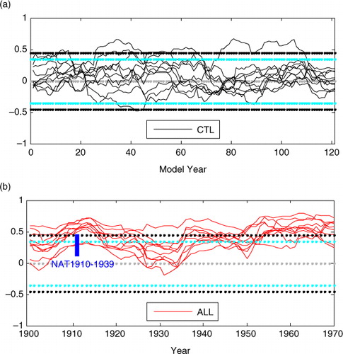
Each experiment consists of five ensemble members, where each member was initialized using the method of taking different atmosphere – but identical ocean – start conditions for the model. The different atmospheric initial conditions for NAT, ANT and ALL were selected from a prior generated 20-d simulation using a daily restart file every 5-d for the five different ensemble members, respectively. It is sufficient to generate ensemble spread on the time scales of interest here as discussed in Collins et al. (2006). Five 150-yr control (CTL) ensembles have also been performed to test the ensemble independence using the same initialization method except the initial atmospheric conditions were selected from the 600 yr pre-industrial control run. Figure 1a shows the 30-yr running inter-correlations of annual Arctic (north to 60°N) mean SAT among the five ensembles in the control run. The 30-yr running inter-correlations are calculated as the equation: , where n = 30, and and s_y are the variable means/standard deviations in the selected 30-yr window period. The five ensembles do not significantly correlate with each other (Fig. 1a). Nearly all correlation coefficients cannot pass the significance test at the 99% or 95% levels. The positive and negative values are evenly distributed around zero. This suggests that our ensemble simulations can sample natural variability by generating five independent ensembles.

Fig. 1 Thirty-year running inter-correlations of the Arctic (north to 60°N) mean SAT annual time series among all five ensemble members (a) in CTL; (b) in ALL. The blue bar in (b) shows the range of the 10 inter-correlation coefficients over the early warming period 1910–1939 in NAT. The black/cyan dotted lines refer to the 99%/95% significance level of the correlation coefficients. The labelled year is the first year to compute the correlation; for example, the values marked at year 1910 represent the correlation coefficients computed from 1910 to 1939.

Total solar irradiance (TSI) forcing is reconstructed based on a ¹⁰Be ice core record (Lean et al., 1995; Crowley et al., 2003). Although there are many volcanic indices which are global averages, there is a clear difference between the effects on the climate of tropical and high-latitude eruptions (Robock, 2000). Therefore, in this study, volcanic aerosol forcing is represented by the monthly optical depths at 0.55 microns in four bands (90°N–30°N, 30°N–equator, equator–30°S and 30°S–90°S) (Crowley et al., 2003) in order to take into account the latitudinal dependence of the eruption location for the climate response. In the experiments, the volcanic aerosols are injected directly into the stratosphere where they can modify both the short-wave and long-wave radiations (Otterå, 2008). This differs from many previous climate models (e.g. IPCC AR4, Solomon et al., 2007) that often simulated volcanic eruptions by modifying the solar constant. By such implementation, the radiation modification caused by volcanic eruptions is more realistically taken into account than by considering only the short-wave radiation changes. When releasing the aerosols directly into the stratosphere, volcanic eruptions in the tropics lead to strong heating of the lower tropical stratosphere by absorption of terrestrial and solar near-infrared radiation, causing an enhanced equator-to-pole temperature gradient and stronger polar vortex (Robock, 2000; Otterå et al., 2010). The annual solar constant anomalies relative to the 1850–1999 mean and monthly solar irradiation changes caused by volcanic eruptions (30°N–90°N) in the 20th century are shown in Fig. 2a.

Fig. 2 (a) Anomalies of annual effective solar irradiation (30°N–90°N) and annual solar constant relative to the 1850–1999 mean and monthly solar irradiation changes caused by volcanic eruptions (30°N–90°N); (b) CO₂ (unit: ppmv), N₂O (unit: ppbv) and CH₄ (unit: ppbv) concentrations; (c) 11-yr running-mean annual-mean surface air temperature (SAT) anomaly in the Arctic (north to 60°N) in observations and BCM simulation; the labelled year is the middle of the 11 yr used for computation.

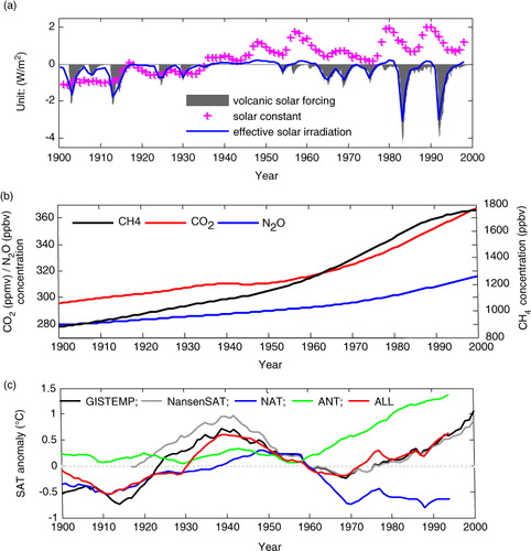
The tropospheric sulphate aerosol forcing is from the historical sulphur cycle simulation (Boucher and Pham, 2002) that was prepared for the IPCC AR4. In the current version of BCM, both direct and indirect effects of tropospheric sulphate aerosols are considered. The indirect effect of tropospheric sulphate aerosols has been parameterized (Hu et al., 2001). The changes in the GHG that are used in the model are the same as those prepared for the EU project ENSEMBLES (van der Linden and Mitchell, 2009) including the annual concentrations of the five most important trace gases (i.e., CO₂, CH₄, N₂O, CFC-11 and CFC-12) during 1850–1999. Figure 2b shows the CO₂, N₂O and CH₄ concentrations in the 20th century used in the ALL and ANT experiments.

2.3. Observational data

In order to compare with the simulated results, several observational datasets were used. The variables which will be compared in the following text include SAT, sea-ice extent and sea level pressure (SLP).

The two observational SAT data used are the NansenSAT and the Goddard Institute for Space Studies (GISS) Surface Temperature Analysis (GISTEMP). NansenSAT is a 2.5°×2.5° gridded monthly SAT dataset for the region north of 40°N from 1900 to 2006 compiled by Nansen International Environmental and Remote Sensing Center, Russia (Kuzmina et al., 2008). The 1200-km smoothing GISTEMP dataset is from 1880, is supplied by the NASA GISS (Hansen et al., 2010), and is provided as the temperature anomaly relative to the base period 1951–1980.

The Zakharov sea-ice data was used for the comparison of the annual variations of the sea-ice extent during the 20th century while HadISST1 was used for the comparison of the climatology distribution of sea-ice extent in different months. The Zakharov sea-ice data are annual mean sea-ice extents in the Arctic from 1900 to 1999. It is a region-averaged dataset and the regions include most parts of the Arctic, leaving out only the eastern Chukchi and Beaufort seas and the Canadian Arctic straits and bays (Johannessen et al., 2004). HadISST1 is the Met Office Hadley Centre's monthly sea-ice concentration and sea-surface temperature dataset on a 1° longitude–latitude grid from 1870 to now (Rayner et al., 2003).

HadSLP2, which is the monthly 5°×5° gridded global SLP anomalies from 1860 (Allan and Ansell, 2006), was used for the analysis on the atmosphere circulation during the relevant period.

3. Results

3.1. The role of internal variability and external forcings

Time series of annual mean SAT anomalies in the Arctic were constructed from NansenSAT, GISTEMP and the model integrations. The regional averages of SAT, sea ice, surface heat flux and surface net long-wave/short-wave radiation will be discussed in the paper. The regional averages of the variables are computed from the area-weighted data in each grid. The simulated variable anomalies are obtained by removing a 600-yr mean of a pre-industrial control run, which is treated as the climatology simulated by BCM. The SAT anomalies in NansenSAT are obtained by removing the 1951–1980 mean, which is the same reference period for GISTEMP. Because in the Arctic regions the NansenSAT contains many missing values in the early period, we use the data after 1912 to compute the anomaly time series, and after applying an 11-yr running mean, the data after 1917 are shown.

The variability and trends of SAT anomalies in ALL are generally in good agreement with the observations both for NansenSAT and GISTEMP (Fig. 2c) in the 20th century. The correlation coefficient is 0.46/0.60 between unsmoothed annual ALL and the unsmoothed NansenSAT (1912–1999)/GISTEMP (1880–1999) time series. These are above the 99% significance level. In particular, the warming trends between 1910 and 1939 (unavailable in NansenSAT because of the missing values in the early period, 0.54°C/decade in GISTEMP and 0.38°C/decade in ALL) and from 1970 up to 1994 (0.27°C/decade in NansenSAT, 0.3°C/decade in GISTEMP and 0.23°C/decade in ALL), as well as the cooling trend between 1940 and 1969 (−0.42°C/decade in NansenSAT, −0.32°C/decade in GISTEMP and −0.32°C/decade in ALL), are all well reproduced (Table 2).

Table 2. The trends of 11-yr running-mean annual-mean SAT in the Arctic (north to 60°N) during selected periods in observations and ALL (unit: °C/decade)

1910–1939	1940–1969	1970–1994
NansenSAT	Unavailable	−0.42	0.27
GISTEMP	0.54	−0.32	0.30
ALL	0.38	−0.32	0.23

Interestingly, the Arctic warming in ALL peaks around 1940, while the temperature evolution in NAT shows a steady warming trend (0.2°C/decade during 1910–1950 and 0.27°C/decade during 1935–1950) until 1950 (Fig. 2c). Thus, it appears that the warming trend between the 1910s and 1940 in ALL can be largely explained by the trend in NAT.

The steady rise in GHG forcing during the early 20th century also likely contributed to a relative warmer background for the temperature variations and specifically from 1930 to 1940 gave a small warming trend (0.22°C/decade) as seen in ANT (Fig. 2c). We also note a slight cooling trend in ANT starting around 1940 and lasting until the late 1950s, likely linked to increased tropospheric sulphate aerosols emissions (Myhre et al., 2001; Boucher and Pham, 2002) and the slightly reduced emissions of CO₂ at the time (Myhre et al., 2001) (Fig. 2b). This could indicate that even though much of the warming trend in ALL between 1910 and 1940 can be largely explained by the trend in NAT, the ANT could play a role in getting the timing of the peak warming correct. As mentioned earlier, the reduced emissions of CO₂ during the 1940s in combination with increased tropospheric sulphate aerosols contributed to a cooling trend from 1940 to the late 1950s. The subsequent solar minimum starting in the late 1950s/early 1960s in combination with the strong volcanic eruptions in the 1960s would have further added to the cooling. The late warming after 1970, on the other hand, is only found in ANT and ALL, indicating that the anthropogenic forcing (i.e., well-mixed GHG) was the primary cause for this warming (Tett et al., 1999; Crowley, 2000; Johannessen et al., 2004).

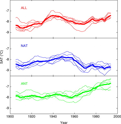
The model results discussed above are robust (Fig. 3), with all five ensembles showing similar trends of SAT during the 20th century in ALL, NAT and ANT experiments.

Fig. 3 Eleven-year running-mean annual-mean Arctic SAT averages in five ensembles (thin lines) and ensemble mean (thick lines) of ALL, NAT and ANT experiments.

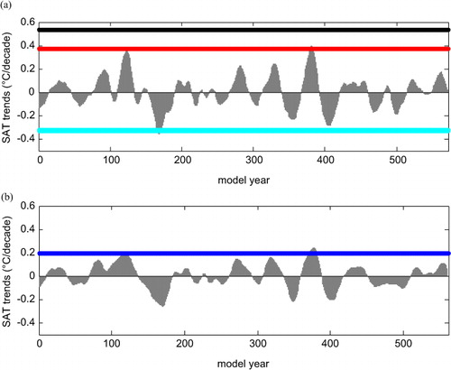
The results presented above are the outcome of coupling between the external forcings and the internal variability. The role of internal variability must be clarified before further discussing the contribution of the external forcings to any warming trend. The early 20th century warming trend lasts about 30 yr in observations and ALL and about 40 yr in NAT. The probability of a strong Arctic warming of similar size as the one in observation, ALL and NAT caused by internal variability has been tested using the 600-yr pre-industrial control run. Figure 4a and 4b shows the 30- and 40-yr running trends of the 11-yr running-mean SAT in this run, respectively. For comparison, the 1910–1939 warming trends in ALL/GISTEMP are shown as the red/black lines in Fig. 4a and the 1910–1949 warming trend in NAT is shown as the blue line in Fig. 4b. It can be seen that the probability of the internal variability simulated in BCM to cause the Arctic warming in the early 20th century is quite low. Only a few running trends can reach the red line and none can reach the black line. The ratios of the running trend exceeding the warming trend during 1910–1939 in ALL and during 1910–1949 in NAT are 0.7% and 1.96%, respectively. The ratios are calculated by dividing the numbers of the year when the trends exceed the trends in ALL or NAT by total year numbers. Therefore, according to our analysis there is little chance to explain a similar or stronger Arctic warming in the 20th century in BCM simply by internal variability alone.

Fig. 4 The running trends of the 11-yr running-mean SAT in 600-yr control run with the running window width as (a) 30 yr and (b) 40 yr. The red/black lines in (a) indicate the 1910–1939 warming trend in ALL/GISTEMP. The cyan line in (a) indicates the 1940–1969 cooling trend in ALL and GISTEMP. The blue line in (b) indicates the 1910–1949 warming trend in NAT (unit: °C/decade).

Although there is a very small probability that the internal variability can cause a similar warming as the Arctic warming in the early 20th century in ALL, we believe it is highly unlikely that the warming can appear in all five ensembles during the same multidecades as shown in Fig. 3, without external forcings in the model. This is because the sampling method ensures generating basically uncorrelated ensemble members as shown in Fig. 1a.

When all the external forcings are included in the model, the 30-yr running correlation coefficients of the annual Arctic mean SAT among all five ensembles are normally positive during the whole of the 20th century (Fig. 1b). During the early warming period, 8 of the 10 inter-correlation coefficients among the five ensembles pass the 99% significance level while the remaining two are slightly below but quite close to the 95% significance level. During the late warming period, for example, all 10 inter-correlation coefficients during the mid-1960s to the mid-1990s pass the 95% significance level. These results show that the external forcings have significant impacts on the climate during these two warming periods. The correlation coefficients in NAT during 1910–1939 are also all positive, with parts of them above the 95% significance level, which indicate that the natural forcings play an important role in the early 20th century Arctic warming.

Thus in the model, the robust early 20th century Arctic warming in the entire five ensembles (0.29/0.4/0.46/0.39/0.35°C/decade, respectively) in ALL can be attributed to the significant impacts of external forcings. The effective solar irradiation rose from the 1910s to 1930s and remained high from the late 1930s to around the 1960s north of 30°N (Fig. 2a). Both the increase in the solar constant and the lull in volcanic activity during this period likely contributed to a rising effective solar irradiation (Fig. 2a). Such variations of the natural forcings led to the warming trend between 1910 and 1949 in NAT and can also explain a large part of the warming trend between 1910 and 1939 in ALL.

However, that does not mean that the internal variability contributed nothing to the Arctic warming in the early 20th century. The warming trends in ALL (ensemble mean) and GISTEMP are 0.38 and 0.54 C/decade, respectively, and the former is about 70% of the latter. It is possible that in reality the internal variability could contribute to the warming to some extent, but the rather small size of ensemble members in BCM simply did not capture a realization in which the internal variability could cause a stronger warming trend in the Arctic in the early 20th century. In summary, the contribution from internal variability should only occupy a small percentage of the warming trend during 1910–1939, and most of the warming (about 70%) is related to external forcings.

3.2. Changes of sea ice, atmospheric circulation and ocean warm inflow

Figure 5a shows the sea-ice extent climatology in the BCM and in HadISST1 for September, December and March. We define the climatology in the BCM as the 600-yr mean from the pre-industrial control run. The climatology in HadISST1 is defined as the mean of the period 1979–1988 (i.e., the first 10 yr after satellite observation utilization). This period was chosen because the data before this period is not as reliable as those after 1979, while the most recent 20 yr data are not a good representation of climatology because of strong sea-ice reductions predominantly caused by global warming (Johannessen et al., 2004; Johannessen, 2008). In the model, sea ice mainly occupies the central Arctic Ocean in September. In December, the sea ice extends and covers the Arctic Ocean, Kara Sea, Laptev Sea, East Siberian Sea, Chukchi Sea, Beaufort Sea and part of the Greenland Sea. The eastern and northern parts of the Barents Sea are also covered by sea ice at this time. By March, the sea ice is reaching its maximum extent and covers most parts of the Barents and Greenland Seas. These distributions are in reasonable agreement with the HadISST1 sea-ice observational data, which supports the ability of the model to capture the realistic features of sea ice in the Arctic despite the model showing relatively larger seasonal variations with less sea ice in September and slightly more in December.

Fig. 5 (a) Sea-ice extent climatology in BCM simulation (white shading, 600-yr mean of a pre-industrial control run) and HadISST1 (solid purple line, 1979–1988 averages) in September (left), December (middle) and March (right); (b) 11-yr running-mean annual-mean sea-ice extent (SIE, left ordinate for model experiments and right ordinate for Zakharov data) variations.

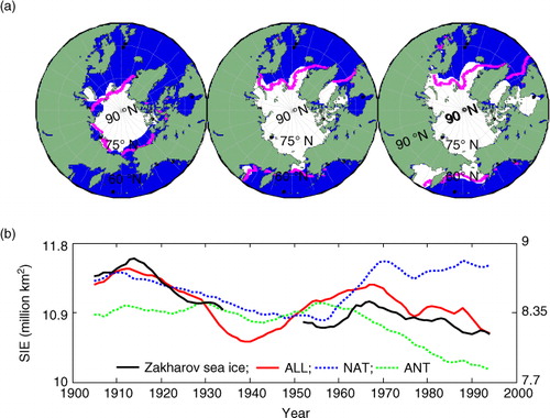
The changes in the Arctic temperatures are largely mirrored by changes in the Arctic sea ice. The sea-ice extent kept decreasing from the mid-1910s to about 1940, while a recovery can be seen from the 1940s to the late 1960s in both the observation and in ALL (Fig. 5b). Nevertheless, the sea-ice variations in the observations and in ALL shown in Fig. 5b are generally in good agreement with a correlation coefficient of 0.42 based on the unsmoothed annual series that pass 99% significance level. The trends of sea-ice extent from 1910 to 1940 are −0.36/−0.16/−0.02 million km²/decade in ALL/NAT/ANT, respectively. This means that the natural external factors (NAT; Fig. 5b) contributed to a large part of the sea-ice loss during the early 20th century Arctic warming period. The anthropogenic factors (ANT; Fig. 5b) contributed little to sea-ice melting during the whole warming period.

Melting and freezing of sea ice play a vital role in the heat exchanges between the ocean surface and the air, especially in sea-ice marginal regions (Screen and Simmonds, 2010). Particularly important in this regard is the well-known ice–albedo feedback (Curry et al., 1995). During the period with direct solar radiation, mainly in summer, intensified solar radiations cause more sea-ice melting. As a result, more ocean surface is exposed. This will in turn allow the upper ocean to absorb more radiation and store more heat, so that more sea ice can be melted because of warmer underlying surface. At the onset of winter, the warm underlying surface will also delay the sea-ice refreezing and at the same time releases more heat into the cold lower troposphere causing SAT to rise.

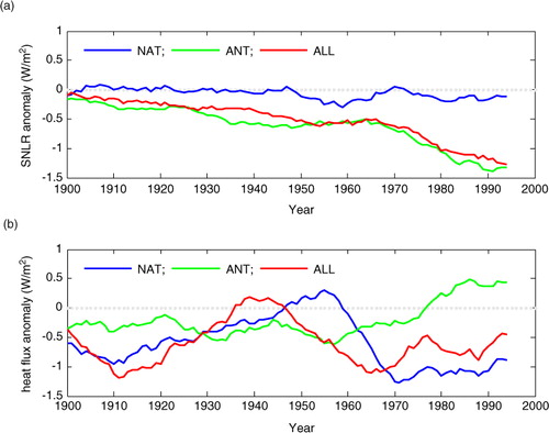
The heat absorbed and contained in the land and ocean can be released by latent and sensible heat flux and long-wave radiation into the air. Net surface long-wave radiation (NSLR, upward is positive) in ALL keeps decreasing in the 20th century and primarily dominated by the trend in ANT (Fig. 6a). On the other hand surface upward heat fluxes in ALL increase from 1910 to 1940, which can be largely attributed to the steady increasing from 1910 until the mid-1950s in NAT (Fig. 6b). Thus, the upward latent and sensible heat flux changes contribute the more heat released from the underlying surface to the air during the 20th century Arctic early warming period.

Fig. 6 Eleven-year running-mean anomaly of simulated annual-mean (a) surface net long-wave radiation (SNLR, upward is positive) and heat flux (latent heat flux plus sensible heat flux, upward is positive) in the Arctic (north to 60°N).

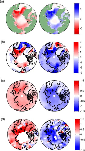
In ALL, the simulated regions with large sea-ice variations are primarily located in sea-ice marginal regions (Fig. 7a) where ocean surfaces are exposed to solar irradiance in summer and covered by sea ice in winter. The largest sea-ice changes are found east of Greenland and Barents Sea, where most ocean areas are exposed to the atmosphere even in December (Fig. 5a). Then the less sea ice and more exposed ocean surface caused obvious variations in the heat exchange between the ocean and the atmosphere through latent and sensible heat flux modifications during 1910–1939/1940–1969 (Fig. 7b). The annual-mean heat flux trends of 1910–1939/1940–1969 are up/down to ±10Wm⁻²/decade in the Barents Sea. The largest annual-mean SAT anomalies (trends over ±1°C/decade) are also found in the Barents and Greenland Seas. The Arctic warming patterns located in the ocean areas in both ALL and the observations (Fig. 7c and Fig. 7d) are very similar to the simulated sea-ice changes (Fig. 7a) and heat flux changes during 1910–1939 (Fig. 7b), indicating a close relationship among the three.

Fig. 7 Trends of annual-mean (a) sea-ice concentration (unit: percent/decade); (b) surface upward heat flux (unit: Wm⁻²/decade); (c) surface air temperature (unit: °C/decade) in ALL forcing run and (d) surface air temperature (unit: °C/decade) in NansenSAT (blank: missing value regions) during 1910–1939 (left) and 1940–1969 (right). We adopt only the grids with more than 20 yr of available observations in NansenSAT in the 30-yr periods from 1910–1939 or 1940–1969 to calculate the trends which are shown in Fig. 6d.

The local solar irradiation changes are potential sources of heat that can explain the simulated Arctic temperature and sea-ice anomalies in the model. In NAT, an increase is found in the surface net short-wave radiation (SNSR) averaged north of 60°N between the 1910s and the 1950s, while a decrease can be seen from the 1950s to about 1970 (Fig. 8a). In ANT, on the other hand, a small decreasing trend of SNSR is seen to start from the beginning of the 20th century lasting until the late 1950s (Fig. 8a). The variations in the SNSR in ALL (Fig. 8a) are quite similar to those in NAT except for the 10-yr advance of the peak. In NAT and ALL, there are significant correlations between the SAT and the SNSR anomalies, with correlation coefficients of 0.84 and 0.52, which pass 99% significance level for NAT and ALL calculated from the original (non-running-mean) data during 1900–1999, respectively, while the correlation between SAT and SNSR in ANT is only 0.18 which does not pass 95% significance level (Fig. 2c and 8a). In the model, the direct radiative effects from natural factors, such as increased solar irradiation and lack of volcanic eruptions, appear to play a crucial role in driving the Arctic early 20th century warming. This confirms that most of the warming in the model is related to the external forcings.

Fig. 8 (a) Eleven-year running-mean anomaly of simulated annual-mean surface net short-wave radiation (SNSR, downward is positive) in the Arctic (north to 60°N); (b) 11-yr running-mean standardized annual-mean Atlantic meridional overturning circulation (AMOC), Barents Sea heat transport (BSHT), Barents Sea ice area (BSIA) with surface air temperature (SAT) in the ALL experiment; trends of sea level pressure in (c) HadSLP2 and (d) ALL (unit: hPa/decade) during 1910–1939 (left) and 1940–1969 (right) (50°N–90°N, 300°W–80°E).

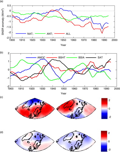
Besides the local irradiance changes, the internal variability and/or external forcings could also cause oceanic and atmospheric circulation changes that can modulate the meridional heat transports. The standardized temporal evolution of the Atlantic meridional overturning circulation (AMOC), the Barents Sea heat transports (BSHT), the Barents Sea ice area (BCIA) and SAT in ALL are shown in Figure 8b. The AMOC is defined as the maximum of the Atlantic stream function between 20°N and 50°N. The BSHT is calculated as the net heat transport (calculated relative to 0°C) between Svalbard and northern Norway (i.e., the Barents Sea Opening) into the Barents Sea. The BSHT gradually becomes stronger after 1920 until reaching a peak value around the mid-1930s. The increased BSHT helps to warm ocean surface and melt sea ice in Barents Sea during this period. According to the model the AMOC consistently strengthens after 1900 and reached its peak around 1930, which could cause the increased BSHT. During 1910–1939, there is an anomalous high located along the south Greenland, Iceland, Scandinavia and western Russia with an anomalous low located in the north of the high (Fig. 8c and 8d). These anomalous SLP patterns can bring more warm air along the southern part of Greenland to northern Norway and Barents Sea and also could drive stronger Atlantic Ocean warm inflow into the far northern oceans, which are consistent with the discussion in Bengtsson et al. (2004).

4. Discussion and conclusions

The model simulations and the analysis on observational data presented in this paper indicate that the intensified solar radiation and a lull in volcanic activity during the 1920s–1950s are the main cause of the early 20th century Arctic warming. The local solar irradiation changes play a crucial role in driving the Arctic early 20th century warming. The meridional heat transport via the ocean and the atmosphere also likely contribute to the warming. When SAT rose, the sea ice melted in Arctic, which let the surface absorb more heat and caused the SAT to rise further. The variability and the anomaly patterns of SAT are largely mirrored by sea-ice changes during the early 20th century.

In terms of the natural forcings, both the solar and volcanic forcings are subject to considerable uncertainty. In the TSI reconstruction used in this study (Crowley et al., 2003), the increased total irradiance over the first half of the 20th century is about 1.8 Wm⁻². This is three times larger than the more recent estimate widely used in CMIP5 (Wang et al., 2005). Another TSI reconstruction (Shapiro et al., 2011) shows about 3.6 Wm⁻² increases during the early 20th century, or roughly six times the values typically used by CMIP5 models. It is worth noting that these reconstructions diverge in the past but agree reasonably well during the satellite observational period. This implies that the observational data do not necessarily allow us to select and favour one of the proposed reconstructions. In order to illustrate the potential importance of the TSI forcing for the early 20th century warming, we compared the global and the Arctic SAT simulated with BCM and the new Norwegian Earth System Model (NorESM; Bentsen et al., 2013). The NorESM uses the low solar forcing of Wang et al. (2005), while BCM uses the intermediate solar forcing of Crowley et al. (2003) during the early 20th century warming period. It is worth noting that the BCM is able to reproduce the early Arctic warming, while NorESM can only give a much milder stable warming signal (figure not shown). It is tempting to speculate that the different solar forcings used are an important reason for this. There may of course be other reasons why BCM2 is able to reproduce past Artic climate change well, while other models, such as NorESM, do not. For example, there may be differences in the relative importance of external forcing and internal variability in models. An important task for future studies will therefore be to disentangle the importance of the various external forcing and internal variability in BCM2, and contrast these against those of the NorESM, which behaves more like other climate models (e.g. IPCC AR4). However, to properly address this issue, additional experiments would need to be done. This is planned for future studies and is beyond the scope of this study.

The estimates of volcanic aerosols in the pre-satellite era also contain uncertainties. Even for the relatively well-documented Krakatau eruption in 1883, global estimates of the amount of aerosols ejected to the stratosphere can differ as much as a factor 4 between different reconstructions (Stendel et al., 2006). The usage of the different reconstructions could also give different output.

Finally, there are also many uncertainties associated to the possible role of tropospheric aerosols for temperature variations in the Atlantic–Arctic region. Shindell and Faluvegi (2009) investigated in detail the sensitivity of regional climate to changes in different aerosol species using a coupled ocean–atmosphere GCM. For the Arctic region, they found that decreasing concentrations of sulphate aerosols and increasing concentrations of black carbon have substantially contributed to the rapid Arctic warming since 1980. In BCM2, only estimates of the tropospheric sulphate aerosols are used. All other aerosol species, such as black carbon, are kept constant at their 1850 levels. The model also does not include a comprehensive treatment of aerosols and atmospheric chemistry like some of the more recent CMIP5 models (including NorESM), but does include a parameterization of the indirect effect of these aerosols.

Separate aerosol only ensemble run members for BCM are planned and will be carried out in the near future. This will allow us to better quantify the role of the sulphate aerosol forcing in the 20th century temperature evolution in BCM. However, this will be done in a future study, and a detailed investigation of this issue is not within the scope of the present paper.

When all forcings are included in the model, the simulated climate changes are realistic, such as Arctic SAT variability and patterns. It is worth noting that the simulated climate changes in ALL cannot be reproduced by simply adding together the individual responses in the NAT and ANT. This suggests that complex non-linear processes could be important in the total climate responses to the combination of the anthropogenic and natural forcings. Further studies on how such variability interacts with different external forcings are therefore clearly warranted.

In summary, the results suggest that external forcings played a prominent role in the early 20th century warming. Moreover, given the potentially important role of natural external forcings for climate variability at high latitudes, their future evolution should also be considered in terms of near-future development of the Arctic (and global) climate. Therefore, different scenarios should be assessed both with respect to TSI changes as well as volcanic eruptions when performing model projections for the future.

5. Acknowledgements

This study has been supported by the Research Council of Norway through the following projects: The ArcWarm project headed by Ola M. Johannessen, the BluArctic project headed by Yongqi Gao and the joint Norwegian-Russion project NORRUS headed by Ola M. Johannessen and by the Program of Supercomputing. This study is also a contribution to the Center for Climate Dynamic (SKD) at the Bjerknes Center for Climate Research.

References

- Ahlmann H. W. S . The present climatic fluctuation. Geogr. J. 1948; 112: 165–193.
- Allan R. , Ansell T . A new globally complete monthly historical gridded mean sea level pressure dataset (HadSLP2): 1850–2004. J. Clim. 2006; 19: 5816–5842.
- Bengtsson L. , Semenov V. A. , Johannessen O. M . The early twentieth-century warming in the Arctic – a possible mechanism. J. Clim. 2004; 17: 4045–4057.
- Bentsen M. , Bethke I. , Debernard J. B. , Iversen T. , Kirkevåg A. , co-authors . The Norwegian Earth System Model, NorESM1-M – part 1: description and basic evaluation of the physical climate. Geosci. Model. Dev. 2013; 6: 687–720.
- Bleck R. , Rooth C. , Hu D. , Smith L. T . Salinity-driven thermocline transients in a wind- and thermohaline-forced isopycnic coordinate model of the North Atlantic. J. Phys. Oceanogr. 1992; 22: 1486–1505.
- Bleck R. , Smith L. T . A wind-driven isopycnic coordinate model of the North and Equatorial Atlantic Ocean 1. Model development and supporting experiments. J. Geophys. Res. 1990; 95: 3273–3285.
- Boucher O. , Pham M . History of sulfate aerosol radiative forcings. Geophys. Res. Lett. 2002; 29: 1308.
- Collins M. , Botzet M. , Carril A. F. , Drange H. , Jouzeau A. , co-authors . Interannual to decadal climate predictability in the North Atlantic: a multimodel-ensemble study. J. Clim. 2006; 19: 1195–1203.
- Crowley T. J . Causes of climate change over the past 1000 years. Science. 2000; 289: 270–277.
- Crowley T. J. , Baum S. K. , Kim K. , Hegerl G. C. , Hyde W. T . Modeling ocean heat content changes during the last millennium. Geophys. Res. Lett. 2003; 30: 1932.
- Curry J. A. , Schramm J. L. , Ebert E. E . Sea ice-albedo climate feedback mechanism. J. Clim. 1995; 8: 240–247.
- Delworth T. L. , Knutson T. R . Simulation of early 20th century global warming. Science. 2000; 287: 2246–2250.
- Déqué M. , Dreveton C. , Braun A. , Cariolle D . The ARPEGE/IFS atmosphere model: a contribution to the French community climate modelling. Clim. Dynam. 1994; 10: 249–266.
- Eythorsson J . Temperature variations in Iceland. Geogr. Ann. 1949; 31: 36–55.
- Furevik T. , Bentsen M. , Drange H. , Kindem I. K. T. , Kvamstø N. G. , co-authors . Description and evaluation of the Bergen climate model: ARPEGE coupled with MICOM. Clim. Dynam. 2003; 21: 27–51.
- Hansen J. , Ruedy R. , Sato M. , Lo K . Global surface temperature change. Rev. Geophys. 2010; 48: G4004.
- Hu R. , Planton S. , Déque M. , Marquet P. , Braun A . Why is the climate forcing of sulfate aerosols so uncertain?. Adv. Atmos. Sci. 2001; 18: 1103–1120.
- Johannessen O. M . Decreasing Arctic sea ice mirrors increasing CO2 on decadal time scale. Atmos. Ocean. Sci. Lett. 2008; 1: 51–56.
- Johannessen O. M. , Bengtsson L. , Miles M. W. , Kuzmina S. I. , Semenov V. A. , co-authors . Arctic climate change: observed and modelled temperature and sea-ice variability. Tellus A. 2004; 56: 328–341.
- Kelly P. M. , Jones P. D. , Sear C. B. , Cherry B. S. G. , Tavakol R. K . Variations in surface air temperatures: part 2. Arctic Regions, 1881–1980. Mon. Wea. Rev. 1982; 110: 71–83.
- Kuzmina S. I. , Johannessen O. M. , Bengtsson L. , Aniskina O. G. , Bobylev L. P . High northern latitude surface air temperature: comparison of existing data and creation of a new gridded data set 1900–2000. Tellus A. 2008; 60: 289–304.
- Lean J. , Beer J. , Bradley R . Reconstruction of solar irradiance since 1610: implications for climate change. Geophys. Res. Lett. 1995; 22: 3195–3198.
- Meehl G. A. , Washington W. M. , Ammann C. M. , Arblaster J. M. , Wigley T. M. L. , co-authors . Combinations of natural and anthropogenic forcings in twentieth-century climate. J. Clim. 2004; 17: 3721–3727.
- Meehl G. A. , Washington W. M. , Wigley T. M. L. , Arblaster J. M. , Dai A . Solar and greenhouse gas forcing and climate response in the twentieth century. J. Clim. 2003; 16: 426–444.
- Myhre G. , Myhre A. , Stordal F . Historical evolution of radiative forcing of climate. Atmos. Environ. 2001; 35: 2361–2373.
- Otterå O. H . Simulating the effects of the 1991 Mount Pinatubo volcanic eruption using the ARPEGE atmosphere general circulation model. Adv. Atmos. Sci. 2008; 25: 213–226.
- Otterå O. H. , Bentsen M. , Bethke I. , Kvamstø N. G . Simulated pre-industrial climate in Bergen climate model (version 2): model description and large-scale circulation features. Geosci. Model Dev. 2009; 2: 197–212.
- Otterå O. H. , Bentsen M. , Drange H. , Suo L . External forcing as a metronome for Atlantic multidecadal variability. Nat. Geosci. 2010; 3: 688–694.
- Overpeck J. , Hughen K. , Hardy D. , Bradley R. , Case R. , co-authors . Arctic environmental change of the last four centuries. Science. 1997; 278: 1251–1256.
- Petterssen S . Changes in the general circulation associated with the recent climatic variation. Geogr Ann. 1949; 31: 212–221.
- Rayner N. A. , Parker D. E. , Horton E. B. , Folland C. K. , Alexander L. V. , co-authors . Global analyses of sea surface temperature, sea ice, and night marine air temperature since the late nineteenth century. J. Geophys. Res. 2003; 108: 4407.
- Robock A . Volcanic eruptions and climate. Rev. Geophys. 2000; 38: 191–219.
- Salas Mélia D . A global coupled sea ice-ocean model. Ocean. Model. 2002; 4: 137–172.
- Screen J. A. , Simmonds I . The central role of diminishing sea ice in recent Arctic temperature amplification. Nature. 2010; 464: 1334–1337.
- Shapiro A. I. , Schmutz W. , Rozanov E. , Schoell M. , Haberreiter M. , co-authors . A new approach to the long-term reconstruction of the solar irradiance leads to large historical solar forcing. Astron. Astrophys. 2011; 529
- Shindell D. , Faluvegi G . Climate response to regional radiative forcing during the twentieth century. Nat. Geosci. 2009; 2: 294–300.
- Solomon S. , Qin D. , Manning M. , Chen Z. , Marquis M. , co-authors . Climate Change 2007: The Physical Science Basis. Contribution of Working Group I to the Fourth Assessment Report of the Intergovernmental Panel on Climate Change. 2007; Cambridge, New York: Cambridge University Press. 996.
- Stendel M. , Mogensen I. , Christensen J . Influence of various forcings on global climate in historical times using a coupled atmosphere–ocean general circulation model. Clim. Dynam. 2006; 26: 1–15.
- Stott P. A. , Tett S. F. B. , Jones G. S. , Allen M. R. , Mitchell J. F. B. , co-authors . External control of 20th century temperature by natural and anthropogenic forcings. Science. 2000; 290: 2133–2137.
- Tett S. F. B. , Jones G. S. , Stott P. A. , Hill D. C. , Mitchell J. F. B. , co-authors . Estimation of natural and anthropogenic contributions to twentieth century temperature change. J. Geophys. Res. 2002; 107: 4306.
- Tett S. F. B. , Stott P. A. , Allen M. R. , Ingram W. J. , Mitchell J. F. B . Causes of twentieth-century temperature change near the Earth's surface. Nature. 1999; 399: 569–572.
- van der Linden P. , Mitchell J. F. B . ENSEMBLES: Climate Change and Its Impacts: Summary of Research and Results from the ENSEMBLES Project. 2009; Exeter, UK: Met Office Hadley Centre.
- Wang Y. M. , Lean J. L. , Sheeley N. R. Jr . Modeling the sun's magnetic field and irradiance since 1713. Astrophy. J. 2005; 625: 522.
- Wood K. R. , Overland J. E . Early 20th century Arctic warming in retrospect. Int. J. Climatol. 2010; 30: 1269–1279.