An approach for tuning ensemble prediction systems

Abstract

Reliable ensemble prediction systems (EPSs) are able to quantify the flow-dependent uncertainties in weather forecasts. In practice, achieving this target involves manual tuning of the amplitudes of the uncertainty representations. An algorithm is presented here, which estimates these amplitudes off-line as tuneable parameters of the system. The tuning problem is posed as follows: find a set of parameter values such that the EPS correctly describes uncertainties in weather predictions. The algorithm is based on approximating the likelihood function of the parameters directly from the EPS output. The idea is demonstrated with an EPS emulator built using a modified Lorenz'96 system where the forecast uncertainties are represented by errors in the initial state and forecast model formulation. It is shown that in the simple system the approach yields a well-tuned EPS in terms of three classical verification metrics: ranked probability score, spread-skill relationship and rank histogram. The purpose of this article is to outline the approach, and scaling the technique to a more realistic EPS is a topic of on-going research.

• ensemble prediction systems
• EPS tuning
• parameter estimation
• state space models
• Bayesian inference

1. Introduction

Ensemble prediction systems (EPSs) are indispensable tools for generating probabilistic predictions of weather and climate (Leutbecher and Palmer, 2008), and they are applied also in many related application areas, such as flood forecasting (Cloke and Pappenberger, 2009). Accuracy of the EPS stems from a skilful high-resolution data assimilation and forecasting system, while its reliability can be attributed to the design of uncertainty representations. By reliability, we mean the capability of a probabilistic system to represent the range of observed events.

Probabilistic prediction systems include representations of initial-state uncertainty and prediction of model formulation uncertainties. The magnitude of the initial-state uncertainty is basically limited by the analysis error covariance, of course assuming in most cases that linear and Gaussian estimation theory holds. However, forecast model uncertainty is less constrained: there are various sources of modelling uncertainty and their relative magnitudes are hard to determine. For instance, the process-based stochastic modelling tends to result in a large number of degrees of freedom in the system. In short, there is lack of practical design criteria for representing the uncertainties in probabilistic systems that would a priori lead to a reliable system. We conclude that tuning the amplitudes of the various components in the uncertainty representation constitutes an estimation problem.

Currently, tuning the relative magnitudes of uncertainty sources typically relies on expert knowledge. The procedure is such that one tests with a combination of initial and model perturbation amplitudes how the system verifies. Depending on the outcome, the trial-and-error procedure is continued. No doubt, with time this leads gradually to a finely tuned system, and experts learn by experience how to tune the system. This is, however, a very costly way to gain the experience; costly in terms of time and, above all, costly in terms of the system potentially being sub-optimal while experience is gathered. Moreover, a critical point is faced when the prediction system components undergo major changes: the system behaviour changes and the subjective component of the procedure may not be valid until new experience is obtained. We argue that an objective tool to guide the tuning process would be a step forward.

In this article, we construct such a tool that is tightly anchored to the theoretical foundations of estimation theory (Durbin and Koopman, 2001). We demonstrate the approach in the context of a modified stochastic Lorenz'96 system (Wilks, 2005), and show that it yields a well-tuned probabilistic system in terms of ranked probability score, spread-skill relationship and rank histogram used as verification metrics. The article is organised such that the estimation approach is derived in Section 2, and the case study is presented in Section 3, before discussion and conclusions.

2. Parameter estimation in state space models

To build the theoretical basis for the EPS tuning approach, let us consider the parameter estimation problem in a general dynamical state space model setup (see, for instance, Durbin and Koopman, 2001; Singer, 2002; Hakkarainen et al., 2012). We write the model at step k with unknown model parameters θ as follows:1 2 3

That is, the probability density of the model state at step k, x _k , depends on the previous state x _k−1 and the values of the model parameters θ via the dynamical forecast model . The likelihood contains the observation model and gives the probability density of observing data y _k , given that the model state is x _k . In addition, we might have some a priori knowledge about the possible values of the model parameters θ, coded into the density p(θ).

The parameter estimation problem in state space models is formulated as follows: estimate the parameters θ, given a series of observations . In the Bayesian parameter estimation framework, the solution to the problem is given by the posterior distribution . The posterior density is proportional to the product of the prior and the likelihood:4

Traditionally, the likelihood density contains a direct comparison between the model and the data. However, in state space models the likelihood needs to be constructed in a different way.

To construct the likelihood, we need the concept of the filtering distribution and the predictive distribution. The filtering distribution at step k is the marginal posterior distribution of the last state vector, , given the whole history of measurements y _1:k and parameter values θ. This distribution is usually the target of different sequential state estimation (data assimilation) methods. The predictive distribution gives the probability density of the predicted state x _k , given all previous measurements y _1:k−1. The filtering distribution can be computed via the Bayes formula by considering the predictive distribution as the prior, which is updated with the most recent data y _k :5

The predictive distribution is computed by propagating the previous filtering distribution through the dynamical model :6

Now, we have all the necessary building blocks for constructing the likelihood density . We start by decomposing the likelihood into the product7

The terms in the product are the predictive distributions of the observations y _k , given the previous observations y _1:k−1 and parameter values θ. These distributions can be computed by propagating the predictive distribution of the model state through the observation model:8

That is, the likelihood in state space models can be computed as a product of predictive densities of observations, which in turn are computed by applying the observation model to the predictive distribution of the model state.

After this general theory, we describe how the method can be implemented in practice, and how it applies to the EPS tuning problem.

2.1. Implementation with various data assimilation methods

The exact way how the likelihood (7) is computed depends on the data assimilation method applied. Here, we discuss how the likelihood computation can be carried out with different methods.

2.1.1. Particle filtering.

Particle filtering (PF) is a fully sampling-based state estimation method that makes no assumptions of the form of the densities of the state vector. In PF, the filtering distribution is described by N samples (particles) drawn from the filtering distribution. Similarly, the predictive distribution is approximated by propagating the particles forward with the dynamical model. The predicted particles are updated with the new observations via importance of sampling, where predicted particles are weighted according to their likelihood; see Doucet et al. (2001) for details about PF methods.

If one has a PF at hand, the likelihood can be computed by writing the likelihood components (predictive distributions of the observations) as expectations over the predictive distribution of the state, and by applying the standard Monte Carlo approximation:9 10 11 where are the predicted particles. In statistics literature, this technique is called the particle marginal approach (Andrieu et al., 2010).

2.1.2. Extended Kalman filtering.

The PF approach can be usable in small-scale state space models, where one can afford to use a large number of particles N, but in high-dimensional systems with a small number of particles, the direct PF approach is known to be impractical. Therefore, one often has to resort to various approximative filtering techniques. One of the most popular methods, suitable for small-to-medium-scale data assimilation problems, is the extended Kalman filtering (EKF), (Kalman, 1960; Smith et al., 1962), which is discussed next.

To introduce EKF, we assume the following specific form for the state space model:12 13

where and are the forecast and observation models, and E _k and e _k are the model and observation errors, respectively. The error terms are assumed to be Gaussians with zero means and covariance matrices Q _k and R _k , respectively.

In EKF, the filtering distribution at step k−1 is Gaussian with mean and covariance matrix :14

The predictive distribution at step k is also Gaussian with mean and covariance matrix 15

where the mean is taken to be the mean of the previous filtering distribution propagated forward with the forecast model: . The covariance matrix of the predictive distribution is computed by propagating the covariance matrix of the previous filtering distribution forward with the linearised forecast model , and assuming that the model error is independent of the model state: .

In the EKF setting, the predictive distributions of the observations, which are the components of the likelihood, are the following:16

where and K _k is the linearised observation model, . Taking the product of these Gaussian densities over step indices k yields the final likelihood:17

where and denotes the determinant. Note that the normalisation constant of the Gaussian density needs to be included, since it depends on the parameters θ. This likelihood formulation was tested for estimating the parameters of a modified Lorenz'96 system in Hakkarainen et al. (2012).

2.2. Other methods

The likelihood computation can be implemented in various other data assimilation systems by changing the way the predictive distributions are computed according to the data assimilation method applied. For instance, in ensemble Kalman filtering methods (Evensen, 2007), the required components in the likelihood can be estimated from the ensemble of predicted states. This approach is taken for instance in Hakkarainen et al. (2013), where the likelihood computation is implemented in the data assimilation research testbed (DART), which uses the ensemble adjustment Kalman filter (Anderson, 2001) as the data assimilation method.

2.3. Applying the approach to EPS tuning

Numerical weather predictions contain uncertainties because of imperfect initial state and forecast model formulation. EPSs account for these uncertainties by imposing clever initial-state perturbations to an ensemble of N forecasts, and randomly perturbing the evolution of each of these forecasts in a specific way (the ‘stochastic physics’). The amplitudes of the perturbations are typically determined by expert knowledge. Here, the aim is to objectively estimate these amplitudes.

EPS systems are, in principle, close to PF systems in the sense that both approximate the uncertainties via samples. The approaches differ in the way the samples are generated: in PF, the importance sampling mechanism is applied, while in EPSs, there are specific techniques for generating the initial-state perturbations and adding perturbations to the model equations (see Leutbecher and Palmer, 2008). From the parameter estimation point of view, however, the same likelihood calculation, given in eqs. (9)–(1), can be applied. In EPSs, the particles are simply the predicted ensemble members and the tuning parameters θ are related to the initial state and model perturbations.

In theory, the ‘best’ way to compute the likelihood would be to use the direct PF approach given in eqs. (9)–(11). However, this is impractical in large-scale (and even in medium-scale) systems, since the ensemble size N is much smaller than the dimension of the state vector, and all predicted ensemble members can easily miss the essential support of the likelihood , making the Monte Carlo approximation meaningless. This phenomenon can be seen even with the 40-dimensional Lorenz EPS emulator studied in Section 3. Therefore, approximations of the likelihood are needed to carry out the likelihood computation.

A straightforward way to approximate the likelihood is to assume a Gaussian form for the predictive distributions, similarly to the EKF approach described in the previous section. Then, the likelihood density assumes the form18

where is the predicted observation, and the covariance matrix describes the uncertainty in the prediction . In EKF, the predicted observation was calculated as , and the covariance matrix was . Correspondingly, in the EPS setting we estimate and the equivalent of (uncertainty of the predicted observation) from the predicted ensemble members in the observation space.

More specifically, consider N ensemble members in the observation space, denoted by , where . Now we use the ensemble mean as and estimate the covariance matrix from the ensemble:19 20

where Y _k contains the centred ensemble members, ).

As the ensemble size is typically very small compared to the dimension of the observation space, it is not advisable to estimate the full matrix . Here, we apply a diagonal approximation for and only estimate the variances of individual observed variables. This is the version of the likelihood we use in our experiments in the next section.

The likelihood (18) has the following intuitive interpretation. If the ensemble spread, described in the formula by , is too small compared to the residuals , the square term in the likelihood will be large and the likelihood low. If the spread is too large, the square terms become small, but the normalisation constant becomes large and the likelihood low. The maximum likelihood is given by a compromise between these two, when the residuals (distance from the prediction to the observations) ‘statistically match’ with the estimated ensemble spread .

3. Case study: tuning a Lorenz EPS emulator

In this section, we present the experiment conducted to test the validity of the likelihood approach for tuning EPS parameters. We test how well the parameter values that give high likelihood perform in terms of three classical EPS verification metrics: the ranked probability score (RPS), spread-skill comparison and rank histogram. We use an EPS emulator built on top of a modified Lorenz'96 system (see Wilks, 2005). We start by briefly introducing the EPS emulator and the validation metrics, and then proceed to the experiment description and results.

3.1. Lorenz EPS emulator

To test the likelihood computation described above, we use an EPS emulator built on top of a modified version of the Lorenz'96 ODE system, described in detail in Wilks (2005). The system used here is similar to the original Lorenz'96 system, but the state variables x _i are affected by forcing due to fast variables y _i , too. The full system that is used for generating the observations is written as21 22

where x _k , k=1,…,K are the ‘slow’ variables that follow the classical Lorenz dynamics (Lorenz, 1996). In addition, each of the K slow variables are forced by a sum of J additional ‘fast’ variables y _j , j=1,…,JK. In our experiments, we use values K=40, J=8, , h=1 and c=b=10, adopted from Leutbecher (2010).

The system (21)–(22) is considered as the ‘truth’ and used for generating synthetic data. The forecast model is run with a larger solver time step, and the effect of the fast variables cannot be therefore directly included. This emulates the common problem in climate and weather modelling: small-scale phenomena cannot be directly modelled and parameterisation schemes need to be developed to describe them. As a forecast model, we use here a version where the average effect of the fast variables is described using a simple parameterisation. In addition, the forecast model contains a stochastic forcing term, which represents the uncertainty due to the parameterisation. The forecast model is written as23

where is the parameterisation in which the missing fast variables y _j are modelled using the ‘resolved’ variables x _k , and is the stochastic forcing term that represents the equivalent of the stochastic physics in this system.

Here, we use a polynomial parameterisation for the deterministic parameterisation:24

In the experiments of this article, we use d=1 and fixed values b ₀=2 and b ₁=0.1, following the results obtained in Hakkarainen et al. (2012), where the objective was to estimate these parameters. The stochastic forcing is given as an independent first-order autoregressive process for each slow variable:25

where is the time step used in the numerical solver (fourth-order Runge–Kutta) and . The stochastic forcing term contains two tuning parameters, the magnitude σ _e and the autocorrelation φ. These ‘stochastic physics’ parameters are what we estimate in the experiment.

The spread of the EPS predictions depends on two things: the stochastic physics and the perturbations made to the initial values from which the predictions are launched. Here, we use a very simple mechanism for sampling the initial values; we draw them from the normal distribution , where are the state estimates computed via EKF. The magnitude of the initial-value perturbations is a tuneable parameter in the EPS system, and is a target of estimation in this article, in addition to the stochastic physics parameters. Thus, in our experiments, we aim at estimating three parameters, .

3.2. Validation metrics

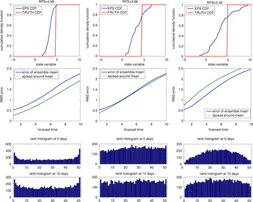
To verify that the proposed likelihood calculation results in well-tuned EPSs, we use three classical EPS validation metrics: RPS, spread-skill comparisons and rank histogram. For completeness, we briefly recall the metrics here (for more details refer to Hamill, 2001; Leutbecher and Palmer, 2008). Examples for all of the metrics, produced by the EPS emulator, are given in Fig. 1.

Fig. 1 The three validation metrics – RPS score (top row), spread-skill comparison (centre row) and rank histogram (bottom rows) – illustrated with an under-dispersive EPS (left column), a rather well-tuned EPS (centre column) and an over-dispersed EPS (right column).

3.2.1. Ranked probability score.

The RPS compares the cumulative density function (CDF) of the truth, which is essentially a step function, to the CDF estimated from the EPS output. Geometrically, the score can be interpreted as the area between the CDF curves. Formally, the metric for a single variable x is26

where P(x) is the CDF of the prediction estimated from the ensemble, and is the CDF of the true state x _T , given as a step function: with and with . In practice, the metric is averaged over selected variables and selected time points. The metric favours situations, where the EPS is tightly spread around the truth. If the EPS spread is too large, the area between the CDF curves is large and a poor (large) RPS value is obtained. On the other hand, if the EPS is over-confident (small EPS spread in the wrong place), the area becomes large as well. The best RPS score is obtained somewhere in between these extremes. The RPS score is illustrated for a single case with different EPS spreads in the top row of Fig. 1. One can see that the score penalises both under- and over-dispersive EPSs.

3.2.2. Spread vs. skill.

In a reliable EPS system, the average spread of the ensemble should match the average forecast error of the ensemble mean; see for instance Leutbecher and Palmer (2008) for a more detailed discussion. The spread of the ensemble is the root mean-squared (RMS) spread around the ensemble mean, and the forecast error is the forecast RMS error compared to the true model state.

Let us denote by s _i , the collection of RMS spreads around the sample mean for a single variable for M different cases (different time instances). The corresponding collection of forecast errors is denoted by , . Then, it is shown in Leutbecher and Palmer (2008) that the RMS spread and RMS error in a perfect ensemble should obey the following relationship:27

where N is the number of ensemble members used to compute the ensemble mean and the RMS spread. The more cases M we have, the more accurately the equation above should hold. That is, the average ensemble mean RMS error should match the RMS spread corrected with a factor that accounts for the finite sample size N. This offers us a way to check how consistent the EPS system is: compare the RMS spread to the forecast RMS error. In the centre row of Fig. 1, the forecast error vs. ensemble spread comparison is illustrated for different EPSs.

3.2.3. Rank histogram.

The third validation metric applied here is the rank histogram, also known as the Talagrand diagram (see Hamill, 2001). The rank histogram is formed by sorting the EPS output for a selected individual variable and checking the rank of the truth in the sorted EPS sample. For instance, in a 10-member EPS, if the truth is outside the ensemble, the rank will be either 1 or 11. If the truth is in the middle of the EPS, the rank is 6.

The ranks are collected for different variables over a certain time period, and histograms of the obtained ranks are drawn. In the ideal situation, if the EPS is well tuned, the histograms should be flat; in the rank sample, there should be roughly equal amount of all possible ranks. To illustrate the metric, rank histograms with various values for the EPS parameters are plotted in the bottom rows of Fig. 1.

3.3. Experiment details

Synthetic observations were generated for the experiment by running the full system (21)–(22), and adding noise to the model output. It was assumed that 24 out of the 40 state variables were observed, with indices 3,4,5,8,9,10,…,38,39,40 (last three variables in every set of five). Noise was added to the model output for these components with standard deviation σ=0.35, and this was used as the data for estimating the EPS parameters.

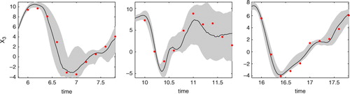
The EPS system was run with ensemble size N=20 in 10 d periods. That is, an ensemble was launched at day 0 and run for 10 d, the next ensemble was launched at day 10 and so on. Daily data were used in constructing the likelihood for each ensemble run. To clarify the EPS setting and the data used in the parameter estimation, ensembles at different time windows for an observed model component are shown in Fig. 2.

Fig. 2 Examples of ensembles launched at different times for the first observed model component (third element in the state vector). The grey envelope is the 95% confidence envelope estimated from the ensemble. Daily observations (red dots) are used for constructing the likelihood.

To study how the likelihood function behaves as a function of the parameters, we conducted the following experiment: 1000 random parameter values were generated uniformly in the interval , and . For each of the parameter values, 200 consecutive ensembles were launched, each 10 d long. The first 30 ensembles were used to construct the likelihood function, and the three validation metrics were computed for each parameter using all of the ensemble runs. For each of the parameter values, the results were averaged over five repeated runs to reduce the randomness in the likelihood.

The state estimates, around which the initial-value perturbations were generated, were computed off-line by running EKF with the stochastic physics turned off.

3.4. Results

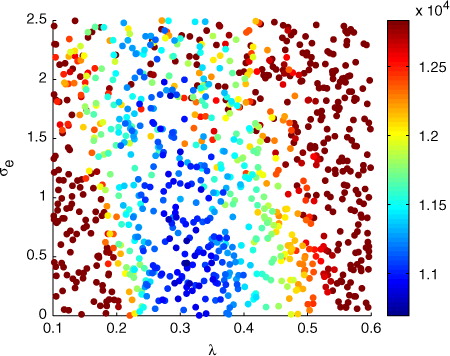
To see how the likelihood surface looks like, we illustrate the parameter samples and negative log-likelihood values with respect to the first two parameters in Fig. 3. The likelihood shows systematic behaviour with respect to the parameters: there is an area with high likelihood values and the function seems to behave rather smoothly around the optimum. In addition, a weak negative correlation between the two parameters is visible (the area of high likelihood values is slightly tilted to the left); a lower value for the initial-value perturbation magnitude means that the stochastic physics magnitude σ _e needs to be increased.

Fig. 3 The negative log-likelihood values for the first two parameters, the initial-value perturbation magnitude and the variance parameter of the stochastic forcing σ _e .

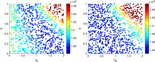
In this case, it seems that the initial-value perturbation magnitude is the parameter that affects the EPS spread the most, and the effect of the stochastic physics parameters is more difficult to see from the samples. To study the stochastic physics parameters further, we repeated the experiment, but with fixed to a certain value. In Fig. 4, the conditional negative log-likelihood with fixed to two different values is given. One can see that the stochastic physics parameters do have a systematic effect, but the exact optimal value for the parameters might be difficult to find. That is, the stochastic physics parameters are not properly identified from data in this experiment; there are many parameter combinations that perform equally well. We wish to note that this behaviour can be specific to this experiment setting, and in more realistic EPS systems the effect of the stochastic physics can be larger compared to the effect of the initial-value perturbations.

Fig. 4 The conditional likelihood values for the stochastic physics parameters with (left) and (right).

Next, we compare how the parameter likelihood measure corresponds to the three validation metrics described in the previous section. Note that the validation metrics are computed from a large collection of EPS runs (200), whereas the likelihood is constructed from a smaller number of ensemble runs (30).

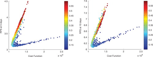
First, we study the correlation between the cost function (negative log-likelihood) values and the RPS score. The results are given in Fig. 5 for 5 d and 10 d predictions. We observe a clear correlation between the two; the lower the cost function value (the higher the likelihood) is, the better the RPS score is. The plots show a peculiar form for the correlation, which has two ‘branches’. The branches are caused by the value of the most significant parameter, the initial-value perturbation magnitude , which is illustrated with colours in the figure; the upper brach consists of too large and the lower branch of too small values.

Fig. 5 Negative log-likelihood values vs. RPS scores. The colours indicate the value of the initial-value perturbation parameter , red means a large value.

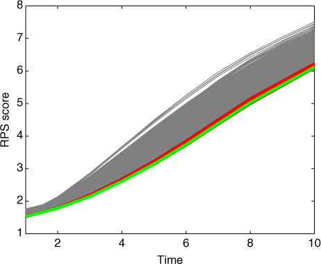
The fact that high likelihood means good RPS scores is further illustrated in Fig. 6. The figure shows all of the different RPS curves for different forecast times computed with the 1000 tested parameter values, and highlights the curves that give high likelihood. From the figure, one can see that a high value for the likelihood corresponds to nearly optimal RPS curves.

Fig. 6 All 1000 RPS curves with different parameter values (grey lines) and the curves corresponding to the best (green) and 10 best (red) parameter values according to the likelihood calculation.

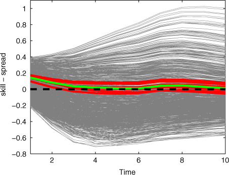
Next, we studied how the parameters that give high likelihood perform in terms of the spread-skill comparison described in Section 3.2.2. In Fig. 7, we show the difference between the ensemble spread and the ensemble mean forecast error, and highlight the curves with high likelihood. The high likelihood values seem to result in a relatively good spread-skill relationship compared to the other tested parameter values. There is a discrepancy in the early forecast range. The reason for this is unknown to us (possibly an effect of spin-up), but on the other hand this phenomenon seems to happen for all other parameter values as well; there is no parameter combination in the 1000 tested parameter vectors for which the spread-skill relationship would hold for the whole forecast range.

Fig. 7 Difference between the ensemble spread and the forecast error of the mean for all 1000 tested parameter values (grey lines) and the curves corresponding to the best (green) and 10 best (red) parameter values according to the likelihood calculation.

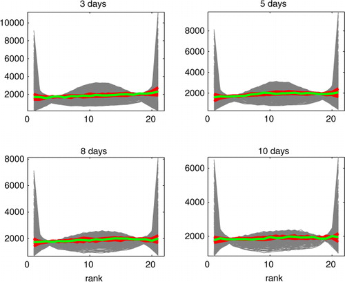
Finally, we compare the rank histograms computed with the parameter values that give high likelihood to all rank histograms obtained with the 1000 tested parameter values. The results are given in Fig. 8. One can see that with the tested parameter values both under- and over-dispersed EPSs were obtained, and the parameters with high likelihood resulted in flat histograms. That is, the likelihood calculation seems to work also in terms of the rank histogram.

Fig. 8 Rank histograms for all 1000 tested parameter values (grey lines) and the curves corresponding to the best (green) and 10 best (red) parameter values according to the likelihood calculation. The four different plots represent different forecast lead times.

4. Remarks and discussion

Traditionally, the tuning of EPS systems is performed manually, applying different EPS validation techniques, such as the three metrics described in Section 3.2. The benefit of the presented approach is that it is objective and relies on observations, whereas in the classical metrics the true state of the model is needed. Obviously, the true state is not available in reality, and it is therefore often replaced with observations or the analysis (state estimate) given by the data assimilation system, both of which contain uncertainties that are not taken into account in the classical validation techniques. In the presented approach, the concept of the ‘true model state’ is not needed.

Fine tuning of initial state and stochastic physics perturbation amplitudes in EPSs is tested here. One has to bear in mind that the work is still on rather conceptual level and the modelling setup is very simplified. Furthermore, the direction of research in representing modelling uncertainties is heading towards individual process-based uncertainty representations. Thus, the number of free parameters in stochastic modelling will increase. This naturally makes the parameter estimation problem harder to solve, especially in limited area EPSs. We believe, however, that the number of the parameters cannot be very high in these models since manual tuning soon becomes intractable. Thus, the study presented here, although not directly up-scalable to realistic systems, is nevertheless relevant in striving towards optimal performance in ensemble prediction. The concept studied here could constitute an ‘off-line’ tuning approach of EPSs: one first attempts to estimate the free system parameters which are tested in a separate and comprehensive posterior validation step.

In this article, we only present how the likelihood function can be computed, and verify that maximising the likelihood yields a well-tuned EPS in a simple case study. We perform a brute-force exploration of the parameter space, and do not discuss how the maximisation of the likelihood function could be done efficiently. Here, 1000 sample points were generated to construct the likelihood surface, where each point represents 30 ensemble predictions with 20 members. With realistic simulation models this is, of course, prohibitively expensive. One clearly needs an effective optimiser that can make use of a small ensemble and few sample points. An additional challenge in the optimisation is that the likelihood is a stochastic function, since it contains random perturbations of the initial values and the model physics. However, methods for optimising random target functions exist, e.g. Kushner and Yin (1997), and we are currently studying techniques that can optimise such a noisy function with as small number of likelihood evaluations as possible. For instance, methods that utilise Gaussian process-based approximations (emulators) of the likelihood surface seem promising (Rasmussen, 2003).

In the example presented here, 30 consecutive 10 d ensemble runs were used to construct the likelihood. However, choosing consecutive ensembles is not necessary, since the perturbations are done independently each time the ensemble is launched. In practice, one could choose a ‘representative’ collection of ensembles, which contains both predictable and unpredictable situations. In addition, since the ensembles are independent, they can be computed in parallel.

5. Conclusions

In this article, we have presented an approach for tuning EPS parameters. The approach is based on approximating the likelihood of the parameters in the state space model setup directly from the EPS output. The method is tested with a Lorenz EPS emulator with three unknown parameters: the initial-value perturbation magnitude and two ‘stochastic physics’ parameters. The performance of the approach is validated by three classical EPS verification metrics: the RPS, spread-skill comparison and rank histogram. The proposed method results in a well-tuned EPS; high parameter likelihood corresponds to good RPS scores, matching ensemble spread and ensemble mean forecast error, and flat rank histograms.

Here, the purpose was to present the EPS tuning concept, and the approach was tested only with a simple small-scale model. We are currently studying how the technique can be scaled up to more realistic EPSs. In addition, we only showed that approximating the tuning parameter likelihood via EPS output makes sense; we did not study how the likelihood can be maximised in practice. Developing such an algorithm – that can handle noisy target functions and requires as few likelihood evaluations as possible – is a topic of on-going research.

6. Acknowledgments

The authors thank Janne Hakkarainen for valuable comments related to the article. The research has been funded in part by the Academy of Finland (project numbers 127210, 132808, 133142, and 134999), the Nessling Foundation, and by the European Commission's 7th Framework Programme, under Grant Agreement number 282672, EMBRACE project (www.embrace-project.eu).

References

- Anderson J. L . An ensemble adjustment Kalman filter for data assimilation. Monthly. Wea. Rev. 2001; 129: 2884–2903.
- Andrieu C , Doucet A , Holenstein R . Particle Markov chain Monte Carlo methods. J. R. Stat. Soc. Ser. B. Stat. Methodol. 2010; 72(3): 269–342.
- Cloke H. L , Pappenberger F . Ensemble flood forecasting: a review. J. Hydrol. 2009; 375: 613–626.
- Doucet A , De Freitas N , Gordon N. J . Sequential Monte Carlo Methods in Practice. 2001; Springer, New York.
- Durbin J , Koopman S. J . Time Series Analysis by State Space Methods. 2001; Oxford University Press, New York.
- Evensen G . Data Assimilation: The Ensemble Kalman Filter. 2007; Springer, Berlin.
- Hakkarainen J , Ilin A , Solonen A , Laine M , Haario H , co-authors . On closure parameter estimation in chaotic systems. Nonlinear Proc. Geophys. 2012; 19: 127–143.
- Hakkarainen J , Solonen A , Ilin A , Susiluoto J , Laine M , co-authors . The dilemma on the uniqueness of weather and climate model closure parameters. Tellus A. 2013. 65, 20147.
- Hamill T. M . Interpretation of rank histograms for verifying ensemble forecasts. Monthly Wea. Rev. 2001; 129: 550–560.
- Kalman R. E . A new approach to linear filtering and prediction problems. J. Basic. Eng. 1960; 35–45. 82 .
- Kushner H. J , Yin G . Stochastic approximation algorithms and applications. 1997; Springer-Verlag, New York.
- Leutbecher M , Palmer T. N . Ensemble forecasting. J. Comput. Phys. 2008; 227(7): 3515–3539.
- Leutbecher M . Predictability and ensemble forecasting with Lorenz'95 systems. Lecture notes, ECMWF meteorological training course on predictability, diagnostics and seasonal forecasting. 2010. Online at: http://www.ecmwf.int/newsevents/training/ .
- Lorenz E. N . Predictability: a problem partly solved. Proceedings of the seminar on predictability, ECMWF. 1996; 1–18. Vol. 1, Reading, UK.
- Rasmussen C. E . Gaussian processes to speed up hybrid Monte Carlo for expensive Bayesian integrals. Bayesian. Stat. 2003; 7: 651–659.
- Singer H . Parameter estimation of nonlinear stochastic differential equations: simulated maximum likelihood versus extended Kalman filter and Ito-Taylor expansion. J. Comput. Graph. Stat. 2002; 11: 972–995.
- Smith G. L , Schmidt S. F , McGee L. A . Application of Statistical Filter Theory to the Optimal Estimation of Position and Velocity on Board a Circumlunar Vehicle. 1962. National Aeronautics and Space Administration (NASA), Technical document.
- Wilks D. S . Effects of stochastic parameterizations in the Lorenz 96 system. Q. J. Roy. Meteorol. Soc. 2005; 131(606): 389–407.