Evaluation of the lake model FLake over a coastal lagoon during the THAUMEX field campaign

Abstract

The THAUMEX measurement campaign, carried out during the summer of 2011 in Thau, a coastal lagoon in southern France, focused on episodes of marine breezes. During the campaign, three intensive observation periods (IOPs) were conducted and a large amount of data were collected. Subsequently, standalone modelling using the FLake lake model was used, first to assess the surface temperature and the surface energy balance, and second to determine the energy budget of the water column at the measurement site. Surface fluxes were validated against in situ measurements, and it was determined that heat exchanges are dominated by evaporation. We also demonstrated that the model was sensitive to the light extinction coefficient at Thau, due to its shallowness and clarity nature. A heat balance was calculated, and the inclusion of a radiative temperature has improved it, especially by reducing the nocturnal evaporation. The FLake lake model was then evaluated in three-dimensional numerical simulations performed with the Meso-NH mesoscale model, in order to assess the changing structure of the boundary layer above the lagoon during the IOPs more accurately. We highlighted the first time ever when Meso-NH and FLake were coupled and proved the ability of the coupled system to forecast a complex phenomenon but also the importance of the use of the FLake model was pointed out. We demonstrated the impact of the lagoon and more precisely the Lido, a sandy strip of land between the lagoon and the Mediterranean Sea, on the vertical distribution of turbulent kinetic energy, evidence of the turbulence induced by the breeze. This study showed the complementarities between standalone and coupled simulations.

• lake modelling
• surface energy budget
• coastal breeze
• water heat storage
• surface temperature

1. Introduction

Land and sea are the main natural surfaces present at the global scale. Lake surface covers only about 3% of continental surfaces (Lehner and Döll, 2004). However, at the regional and local scales, the lake surface can be very large, as is the case in Northern Europe, Asia and North America. The high density of lakes in these regions may affect the regional climate (Balsamo et al., 2012; Kheyrollah Pour et al., 2012). In particular, on summer days, the presence of a lake tends to stabilise the atmosphere, in contrast with land, where turbulence tends to develop. This property is mainly due to the high thermal inertia of the water, which therefore takes more time to warm up or cool down than the continental surface layer. Over the past 10 yr, studies have been conducted to attempt to represent the physical properties of lakes in meteorological and climate models more accurately. Until recently, numerical weather prediction and climate models have represented lakes in a very simplified way.

Indeed, most of the time, the surface temperature of the fraction of lake was fixed during a forecast and therefore did not evolve, whereas in certain circumstances the water temperature can vary significantly, even at a daily scale: for example, due to a strong solar energy supply in the absence of clouds or at night by radiative cooling (Fritz et al., 1980) or by evaporation due to strong wind events (Finch and Calver, 2008). Thus, numerical models of varying complexities have been developed to better represent and understand the coupling between the atmosphere and a lake. Studies performed with regional climate models (Hostetler et al., 1994; Krinner, 2003; Samuelsson, 2010) have highlighted the impact of the inclusion of lakes, especially in studies of climate change impact, showing that lakes bear evidence of climate change. This is confirmed by Schneider and Hook (2010), who found a lake surface warming (1985–2010) for the world's largest lakes, at a mean rate of 0.45° per decade and 0.5° per decade for satellite-based in situ records, respectively. Kjerfve (1994) has proposed a synthesis aiming at describing various components of coastal lagoons, such as for instance, their geomorphology, the involved physical processes (see also Smith, 1994) or the monitoring of ecosystems. Most of the studies conducted over the Mediterranean coastal lagoons aimed at monitoring the aquatic flora and fauna (Perez-Ruzafa, 2007; Derolez et al., 2013). However, environmental issues related to air quality were the source of an increasing number of studies (Flocas et al., 2009; Kanakidou et al., 2011). But only a few studies involving the interaction with meteorology have been carried out on lakes with a small surface area at the Mediterranean coast. Banas et al. (2005) studied the radiation affecting the water column of a lagoon in the south of France, under specific wind conditions. They demonstrated high daily timescale variability of the suspended solid concentrations and the underwater photosynthetically active radiation (PAR) for wind-exposed lagoons, and the need for continuous measurements of irradiance when estimating the mean irradiance in the water column.

Bulk lake models such as FLake (Mironov, 2008), which are being implemented in numerical weather prediction (NWP) and climate models, are not designed to represent the so-called skin temperature depression, the result of the existence of a millimetre-thick surface layer in which viscous effects dominate and heat transfer is via molecular, not turbulent, mixing processes. The temperature of the skin layer is typically a few tenths of a °C lower than the water temperature a few centimetres below, but some studies indicate that the difference may be larger (Garrett et al., 2001), particularly in warm lakes. More observational studies are needed in order to develop algorithms suitable for relating the bulk and skin temperature of lakes, which will be important for improving both the retrieval of surface temperatures from satellite data (Hook et al., 2003) and the representation of the surface temperature in NWP models.

Among the 30 ponds of the Mediterranean coast in Languedoc-Roussillon, the Thau lagoon is the largest (75 km²) and deepest. In addition to its ecological importance, this coastal ecosystem is a resource exploited by various economic activities including aquaculture, boating, fishing, port activities and recreation.

The aims of the study, that combined instrumental and modelling aspects, are as follows:

1. Validate the computation of surface fluxes in FLake with an off-line simulation and in situ forcing. Then evaluate the energy budget of the water column, derived from the observations or computed by the model, and finally evaluate the sensitivity to using a radiative temperature in the computation of the energy budget.

2. Evaluate the sensitivity of FLake to the extinction coefficient, and compare the measured and optimal extinction coefficients: indeed, several studies (Kourzeneva and Braslavsky, 2005; Kourzeneva, 2010; Salgado and Le Moigne, 2010) have shown depth to be the most important parameter for ensuring satisfactory model behaviour. Because of the shallowness of the Thau lagoon and its clarity, the attenuation of light plays an important role in the energy balance of the water column.

3. Highlight the first time ever when the atmospheric model Meso-NH (Lafore et al., 1998) and FLake models are coupled, and evaluate the importance of using FLake model in the coupled simulations and the ability to forecast a sea-breeze event, especially focusing on the boundary layer height over the lagoon and on screen variables over land.

4. Evaluate the sensitivity of accounting for the Lido in the coupled simulation, particularly through its impact on the turbulent kinetic energy.

2. Materials and methods

2.1. Study area

Located at the city of Sète (43°24′N and 3°41′E, GMT + 2 in summer), the Thau lagoon appears to be one of the widest (75 km²) lagoons of the Mediterranean coast, about 17-km long and 5-km wide, and northeast to southwest oriented. The lagoon is separated from the Mediterranean Sea by a 1 km-wide strip of land, known as the Lido. The maximum height of the Lido does not exceed 1.5 m. The eastern part of the lagoon is 11-m deep, and the average depth is 4 m. This 4-m depth will be used as the Thau lagoon depth for the whole study. The lagoon is connected to the sea through several channels, and for that reason, the salinity of the lagoon is rather high and varies seasonally from 29 to 40‰, depending on precipitation rates, evaporation and runoff. However, salinity will not be accounted for in this study. The water is rather clear, reflecting a weak turbidity.

2.2. Continuous measurements

The system of instrumental measurements of the Thau lagoon is composed of the Sète station, which is part of the French network of meteorological observations managed by Météo-France, and Marseillan table, an experimental platform used for monitoring the growth of oysters, located among the oyster tables in the southwestern part of the lagoon. The instrument characteristics are described in Table 1. Measurements of surface pressure and precipitation are collected continuously at the Sète station. Measurements made at the Marseillan table are the air temperature and humidity at 4 m above the water surface, the wind speed and direction at 6 m and the incoming and outgoing longwave and shortwave radiations. These observations complement those of Sète and constitute a data set that can be used to force surface models.

Table 1. List of observables and description of the sensors characteristics

Observable (Height)	Sensor – model	Sampling	Resolution/accuracy
Sète station	Air pressure	Vaisala-PTB220	3600 s	0.5 hPa
Precipitation	Précis Mécanique – PM 3030 tipping bucket rain gage 1000 cm^2	360 s	0.2 mm
Marseillan table	Wind speed and direction (6 m)	Young – Wind monitor 05103	2 s–60 s average	0.3 m s^−1 – 3 °
Air temperature (4 m)	Atexis – platinum wire 1000 Ohm/class A. Socrima radiation shield	10 s–60 s average	0.5°C
Air humidity (4 m)	Vaisala – HMP45 hygrometer. Socrima radiation shield	10 s–60 s average	3%
Longwave and shortwave radiation	Kipp and Zonen – CNR1 radiometer	10 s–60 s average	10% of daily total
Water temperature (−10 cm)	Atexis – Platinum wire 1000 Ohm/class A	10 s–60 s average	0.1°C
Water temperature profile	Chauvin Arnoux – Platinum wire 100 Ohm class A	10 s–60 s average	0.1°C
Fast-response temperature (5 m)	Gill – HS50 sonic anemometer	25 Hz	0.05°C
Fast-response 3D wind (5 m)	Gill – HS50 sonic anemometer	25 Hz	0.01 m s^−1
Fast-response water vapour (5 m)	Licor – 7500 infrared gas analyzer	20 Hz	0.1 g kg^−1
Turbidity	YSI-6600	1800 s	2%
Ifremer boat	Radio-sounding (0–4000 m)	Vaisala – RS92SGP – Humidity – Temperature – Pressure – Wind speed – Wind direction	2 s/10 m	5% 0.5°C 1 hPa 0.15 m s^−1 2°C
Surface reflectance and solar irradiance	Spectroradiometer – FieldSpec UV/VNIR (ASD)	1800 s–3600 s	3 nm / 5% from 400–900 nm
Inwater solar radiance profile	Spectroradiometer – FieldSpec UV/VNIR (ASD) + optical cable	Approx. 9000 s	3 nm / 5% from 400–900 nm
Turbidity	HACH – 2100 N IS	On request	2%

Measurements of water temperature near the surface (−10 cm) have also been performed continuously at the Marseillan table. They will be used to validate the numerical simulations. The IFREMER laboratory (Institut français de recherche pour l'exploitation de la mer) installed a turbidimeter to track the turbidity of the lagoon continuously, affecting the penetration of solar radiation in the water. This device, installed at 1.5 m depth below the water at the Marseillan table, was almost not influenced by the daylight, because a cover protected its internal source of light.

These data were complemented by the installation of an eddy-correlation (EC) station measuring wind, temperature and humidity at a high frequency, allowing, in particular, the calculation of surface fluxes. The sampling frequency of 20 Hz for moisture was re-sampled by interpolation at 25 Hz, the frequency used for wind and temperature. The algorithm describing the calculation of the surface fluxes from measurements is detailed in Bessemoulin (1993) and was used for 20 yr in many measurement campaigns in which the laboratory has participated, such as Carbo-Europe (Noilhan et al., 2011) and Bllast (Lothon et al., 2012). The first period, during which an EC station was set up, extends from March to October 2009, time over which Bouin et al. (2012a) quantified the long-term heat exchanges over the Thau lagoon. But the primary objective was to validate the surface turbulent fluxes, calculated from observations, against those recorded by scintillometers, installed on each side of the lagoon (Bouin et al., 2012b). The second period, ranging from 6 August to 3 October 2011 (hereafter referred to as the THAUMEX period), coincides with the THAUMEX experiment, in which turbulent surface fluxes were used to validate the numerical simulations. The sign convention for fluxes is such that a flux is considered positive from the surface to the atmosphere and also from the bottom of the lagoon to the sediment layer.

2.3. Intensive observation periods

Three intensive observation periods (IOPs) were conducted during THAUMEX to document sea breezes, a frequent meteorological but also classical boundary layer phenomenon in this region during the summer. The assessment of the weather situation and the probability of breeze occurrence was evaluated on a regular basis in consultation with the weather forecast service of the Hérault region. When a sea breeze was expected, and the logistical requirements filled, such as the availability of the boat and its pilot, the decision to perform an IOP was taken and the team responsible for carrying out the measurements went on-site. Radio-soundings with Vaisala RS92SGP sondes were launched from the boat, moored to the platform, every 3 hours from sunrise until late afternoon, when the breeze was well established, to gather information on the vertical profiles of air temperature, humidity and wind and describe the atmospheric boundary layer (ABL).

The IOP2 on 30 August 2011, which appeared to be the less cloudy IOP day and the more representative of a breeze event, from land breeze in the morning to sea breeze in the afternoon, is more widely presented in this article. In fact, during IOP1 on 24 August 2011, low-level clouds developed in the morning over land and were advected over the lagoon. Conversely, during IOP3 on 2011 September 21, a veil of cirrus cloud invaded the sky. The presence of clouds during IOP1 and IOP3 was more difficult to model, therefore only IOP2 was modelled.

Furthermore, radiometric measurements were performed during IOP1 and IOP2, with a portable Spectroradiometer (FieldSpec UV/VNIR from Analytical Spectral Devices Inc.), across the spectral range 325–1075 nm with a spectral resolution ranging from 1 to 3 nm. The integration time was chosen automatically by the spectroradiometer depending on the intensity of the incoming radiation. Measurements of water-leaving spectral reflectance and solar spectral irradiance were performed around every half hour. To facilitate operation in the underwater environment, an optical cable was linked to the bare head of the spectroradiometer with a field-of-view (FOV) of 22°, as explained in Potes et al. (2013). Measurements of underwater spectral radiance were performed approximately every 2.5 hours. The quality of the spectral measurements during IOP2 appeared to be unusable, mainly due to the degradation of the device. Therefore, their analysis relied exclusively on IOP1.

2.4. Measurements, meteorological conditions and water turbidity

Not all measured parameters were available for all time periods. The data set ranging from April 2008 to December 2009 was described in Bouin et al. (2012a), and it will not be discussed here. Only observations over the THAUMEX period, made between 6 August and 3 October, 2011 are presented.

2.4.1. Water temperature.

For the purposes of the THAUMEX campaign, a special device for temperature measurement at different depths was developed. Three floats connected by metal tubes, forming a triangle, were used to support 13 temperature sensors (Fig. 1) arranged along a cable between the near-water surface and the bottom of the lagoon. The vertical resolution was higher near the surface, with half of the sensors in the first metre of water. Some sensors drifted over time or stopped working; in such case, the corresponding recorded data were discarded. Failing sensor data were interpolated vertically on a finer grid, with a resolution of 5 cm, in order to have a continuous space and time series at our disposal, for subsequent comparison with the results of numerical simulations. During the THAUMEX period, the mean temperature <T> of the water column was 24°C, and it was calculated according to the following equation:1

Fig. 1 Device for measuring the temperature profile. The picture shows the device structure and the measurement depths from 10 cm to 4 m are indicated below.

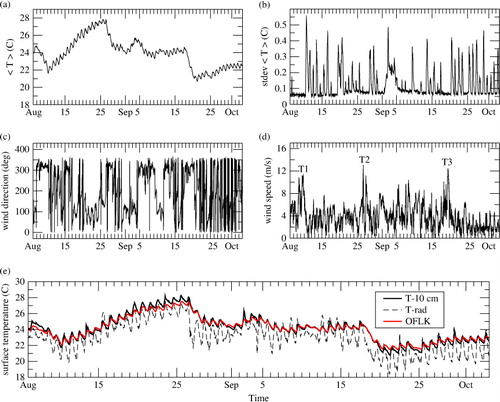
As illustrated in Fig. 2a, it varied from a minimum of 20.7°C on September 20 to a maximum of 27.8°C on August 27. The related standard deviation is rather small: 0.12°C on average over the period, with values ranging from 0.04 to 0.56°C (Fig. 2b). Three episodes lasting 2 to 3 d are noteworthy because they were associated with a significant decrease of the water column temperature. Thus, during these periods, centred around August 9, August 28 and September 19, the average water temperature has decreased by 2.7, 3.3 and 3.6°C, respectively.

Fig. 2 For the THAUMEX period: (a) vertical mean water column temperature <T>, (b) standard deviation of <T>, computed from profile measurements. Measured wind direction (c) and wind speed (d), T1, T2 and T3 indicating the Tramontana events. (e) 3 Hourly running average of temperature measured at −10 cm (solid black), radiative temperature calculated from radiation measurements (dashed black) and surface temperature modelled with the OFLK calibrated FLake configuration (red).

2.4.2. Wind.

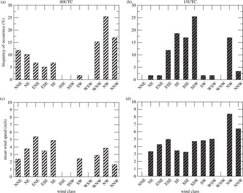
The decrease in water temperature is due to episodes of tramontana, as shown in Fig. 2c–d, a north north-westerly wind that is relatively intense in the Mediterranean region. The THAUMEX period is also characterised by the development of sea breezes, during which the wind moves to the south during the day. The presence of breezes during August and September is demonstrated on the wind-field-averaged daily cycle and shown in Fig. 3 by its hodograph: for example, the point at 15 UTC indicates that the wind is coming almost from the south. The average was computed over the THAUMEX period. It highlights the fact that between 21 UTC and 09 UTC, the wind is oriented to the north, which corresponds to the nocturnal breeze settling when the continent is cooling after sunset, and also to northerly winds such as the tramontana or mistral. The sea breezes rise on average around 11 UTC and drop in intensity from 18 UTC, gradually rotating clockwise. Their intensity is on average lower than the northerly winds. This is confirmed in Fig. 4, where the wind has been classified by sectors of 30°, which represents the distribution of frequencies of occurrence and the average wind speed for each class. Indeed, at night, the wind is most often oriented to the north (Fig. 4a) with average speeds ranging from 2 to 5 m s⁻¹ (Fig. 4c), while in the afternoon (Fig. 4b), nearly 70% of the atmospheric circulation comes from the south, the result of summer sea-breeze regimes with wind speeds ranging from 3 to 8 m s⁻¹ (Fig. 4d).

Fig. 3 Hodograph of daily mean wind over the THAUMEX period. Numbers indicate UTC times.

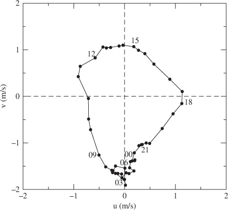
Fig. 4 Histograms of frequency of occurrence at 00 UTC (a) and 15 UTC (b) and mean wind speed at 00 UTC (c) and 15 UTC (d) for wind classes where direction was divided into 12 sectors of 30° each.

2.4.3. Air temperature and humidity.

Very few rainfall events occurred during the THAUMEX period, which was characterised by a relatively warm air temperature. The daily average air temperature was 22°C, with a maximum of 26.1°C in mid-August and a minimum of 17.2°C at the beginning of October. Above the lagoon, the air also exhibits large variations in specific humidity. During calm periods, the air warming induces an increase in evaporation, leading to a significant increase in specific humidity. This is the case in August for example, when the humidity amplitude is about 0.012 kg kg⁻¹, whereas in early October, the same amplitude is about half as strong.

2.4.4. Radiative components and skin temperature.

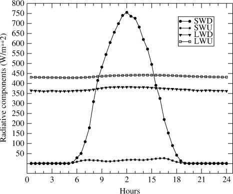
The average daily cycle of radiative components, where the variables were averaged at the time of measurements (here, every half hour) over the whole period is presented in Fig. 5. It indicates that the study period was dominated by strong solar radiation (maximum of 750 W m⁻²) and therefore a lower average cloud cover, which is consistent with the meteorological observations in the region. The components of the infrared radiation, have, in turn, a slightly marked daily cycle: the incoming radiation ranges from 360 W m⁻² at night to 380 W m⁻² during the day, whereas the outgoing radiation ranges from 429 W m⁻² at night to 442 W m⁻² during the day. The net longwave radiation is written as:2

Fig. 5 Average daily cycle of radiative components: shortwave downward (SWD) and upward (SWU), longwave downward (LWD) and upward (LWU), measured at the Marseillan table.

where LWD and LWU are respectively the incident and outgoing infrared radiation, T _s is the surface temperature, ɛ the water emissivity and σ the Stefan–Boltzmann constant. Assuming an emissivity of 0.97, we can estimate the radiative surface temperature of the water from the measurements and eq. (2) for the THAUMEX period. Figure 2e shows a comparison between the radiative temperature and the observation near the surface. It indicates that measurements of the temperature at −10 cm below the surface do not drift over time. Figure 2e also shows that the radiative temperature is far colder than the −10 cm deep temperature. The difference between the radiative, or skin, temperature and the water (bulk) temperature a few centimetres below the surface is often called the skin temperature depression, ΔT. The skin temperature is usually lower than the bulk water temperature because the bodies of water lose energy at the surface layer, a thin layer with a thickness of the order of several millimetres. According to Boyle (2007), ΔT generally lies between −0.2°C and~−1°C, but it has been recorded below −2°C (e.g. Garrett et al., 2001; Harris and Kotamarthi, 2005). These authors compared observed ΔT's from 15 data sets from lakes and reservoirs and found an average value of −0.7°C, and an extremum value of −2.5°C at a 13-km² warm lake near Fort Worth, Texas. The skin temperature depressions tend to be larger at night and at higher water temperatures; during the day, the skin temperature approaches and may even exceed the bulk temperature (Hook et al., 2003).

On average, for the entire THAUMEX period, we obtain ΔT= − 1.0°C. During the night (21–3 UTC), the depression increases to ΔT= − 1.5°C, whereas in daytime (9–15 UTC), the skin temperature approaches the bulk (−10 cm) water temperature, with ΔT= − 0.3°C. These values are within the intervals found in the literature, although they appear to be slightly too large, especially at night. It should be noted that the computation of the radiative temperature is sensitive to the emissivity: a simple sensitivity test shows that the mean nighttime radiative temperature changes by approximately 0.5°C, from ɛ=0.95 to 0.99.

For the two-layer lake model used in this study, it is more consistent to use the −10 cm temperature both as a representation of the water surface temperature and in comparison with the numerical simulations. The radiative temperature will be used to force the computation of surface fluxes using the same formulations employed by the surface model and therefore to evaluate the importance of taking into account the skin surface temperature.

2.4.5. Light extinction coefficient.

The extinction coefficient of light in water is the sum of the absorption of water itself and/or scattering by particles suspended in the water column. The method used to retrieve the extinction coefficient of the water column was based on measurements of inwater solar spectral radiance at several levels deep. Assuming that the spectral downwelling radiance L _d (λ, z), function of the wavelength λ and the depth z, declines exponentially with depth, the attenuation coefficient k(λ), usually referred to as the extinction coefficient, can be determined through the Bouguer–Lambert law:3

The symbol 0⁻ indicates the immediate subsurface level. The underwater downwelling radiance at different depths was measured with a portable spectroradiometer linked to an optical cable with a FOV of 22° (Table 1). Measurements were performed during IOP1 from the IFREMER boat at the Marseillan table [0830 and 1745LT (local time)] and at two other specific points of Thau lagoon near ‘Bouzigues’ (1230 and 1530LT). The profiles were composed using measurements from 0.25 to 3.50 m with a vertical resolution of 25 cm in the first metre and 50 cm afterwards. One of these profiles is shown in Fig. 6a for IOP1 at 1745LT.

Fig. 6 (a) Measurements of underwater spectral radiance at several levels deep taken from the IFREMER boat at the Marseillan table for IOP1 (1745 local time) and (b) spectral extinction coefficient obtained from these measurements.

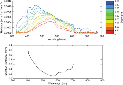
The spectral behaviour of the extinction coefficient is similar for the four cases, with a minimum near 565 nm increasing for shorter and longer wavelengths, as seen in Fig. 6b. For pure water, the minimum of extinction appears around 450 nm (e.g. Smith and Baker, 1981). For wavelengths greater than 700 nm, a similar behaviour is noted for pure water and the four cases studied.

The extinction coefficients were averaged for the 400–700 nm spectral range, frequently called PAR and presented in Table 2. The values for the IOP1 profiles vary from 0.31 to 0.88 m⁻¹, with an average value of 0.52 m⁻¹. Note that the PAR extinction coefficient for pure water is 0.16 m⁻¹.

Table 2. PAR extinction coefficients calculated through eq. (3) for IOP1 (24 August 2011)

Date (local time)	Place	K d (PAR) (m^−1)
2011/08/24 – 08:30	Marseillan	0.88
2011/08/24 – 12:30	Bouzigues	0.53
2011/08/24 – 15:30	Bouzigues	0.31
2011/08/24 – 17:45	Marseillan	0.37

PAR, photosynthetically active radiation.

2.4.6. Water-leaving reflectance and solar irradiance.

The water-leaving reflectance was measured with the portable spectroradiometer with 10° FOV lens foreoptic. Measurements of the water-leaving spectral reflectance were performed from the IFREMER boat at the table of Marseillan and at other points of Thau lagoon during IOP2. All the spectra present a maximum around 565 nm and a peak near 680 nm. The effect of chlorophyll-A absorption, centred on 430 and 660 nm, is clearly visible, leading to a decrease in reflectance around the same wavelengths.

These field measurements were then compared with satellite data. Seven field measurements were selected in accordance with the minimum time lag between measurement and satellite overpass. Satellite radiance of the nearest pixel was corrected for the atmospheric effects in order to have only the water-leaving reflectance (Potes et al., 2011). Aerosol characterisation and water vapour concentration were obtained from Avignon CIMEL (43.9327°N; 4.8777°E), connected to AERONET and located approximately 100 km from Thau lagoon. MERIS level 1 data were used (15 spectral bands). Field measurements and satellite-derived water-leaving reflectance were compared. The correlation coefficient was 0.56, with a root mean square error (RMSE) of 0.0063 W m⁻² sr ⁻¹ nm⁻¹. The points where the satellite fails with higher reflectance than that measured by ground-based spectral measurements correspond to the blue part of the spectrum. This spectral zone somehow presents a sea behaviour (higher reflectance in the blue), which was not observed in the field. This fact can be attributed to neighbourhood pixel contamination, as the distance to the Mediterranean Sea is small (less than 1 km).

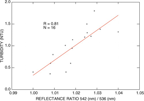
The water surface spectral reflectance is very important in the way that we can have information about the behaviour along the visible and near-infrared parts of the electromagnetic spectrum. This spectral signature allows for the estimation of water constituents and turbidity. Wavelength ratios of field water-leaving surface reflectance were correlated to water turbidity measurements from IFREMER in a total of 16 points. Figure 7 presents the best correlation obtained with the ratio of 542–536 nm (0.81). The reflectance in this spectral region increases towards the maximum at 565 nm. Potes et al. (2012) showed a high correlation (0.96) between the water-leaving reflectance ratio 560–412.5 nm and water turbidity for the Alqueva reservoir. The scatter plot for the ratio at or near the wavelengths of Potes et al. (2012) was performed and presented a lower correlation with respect to the one presented here.

Fig. 7 Scatter plot between field water-leaving reflectance ratio (542/536 nm) and water turbidity (turbidimeter type: HACH 2100N) for IOP2.

The THAUMEX field campaign also includes measurements of the solar spectral irradiance (180° FOV), performed from the IFREMER boat at the Marseillan table and at other points of Thau lagoon on August 30. A remote cosine receptor was used for measuring full-sky irradiance. The measurements (not shown) exhibit the signature of gas absorption, namely oxygen (760 nm) and water vapour (930–950 nm). A detailed analysis of these data is beyond the scope of this article.

2.4.7. Energy budget components.

Knowledge of surface heat fluxes is a prerequisite for the calculation of the heat balance of water. The water column energy budget at the Marseillan site was then computed based on the following equation and assuming no heat advection:4

where ρ _w and C _w are respectively the water density and specific heat and QN is the surface net radiation, composed of the shortwave and longwave incoming and outgoing radiative components, respectively SWD, LWD, SWU and LWU. The energy flux through the bottom sediment is denoted as QB. I(D) is the amount of solar energy that reaches the bottom of the lake at the depth D and follows a Beer–Lambert law (eq. [1]), which in broadband form is written as:5

α _w and k being the albedo and the extinction coefficient of the water, respectively. In eq. (4), the reflection of solar radiation at the bottom is neglected, assuming that solar energy I(D) is entirely absorbed by the sediment layer. The left-hand side of eq. (4) represents the water column heat tendency computed from the mean temperature. It represents the energy balance between the lagoon surface and bottom.

2.4.8. Boundary layer height.

To use the same calculation for the temperature data discretised on the model grid and observed by the balloon, we first calculated the integral mean temperature from the surface to the height h(i), for each model level (or each level of measurement) i, and defined as:6

Next, the boundary layer height was attributed to the layer i when the temperature θ(i) was greater than the average temperature <θ(i)> (eq. [6]) for more than the predefined threshold of 0.25 K (Canut et al., 2012). This simply reflects the fact that the top of the boundary layer is characterised by a strong temperature gradient.

2.4.9. Data over land.

Observations from the French operational observation network were compared to the 1-km mesh model results, in terms of hourly biases and RMSEs. About 90 meteorological stations were available for 2-m temperature, 50 for humidity and 40 for wind (see Fig. 8). These are stations of several types, human observation stations and automatic meteorological stations. The observation network density is quite high and provides an accurate representation of near-surface variables.

3. Model description and setup

3.1. Off-line simulations

The model used in this study to represent the evolution of the water surface temperature of the Thau lagoon is the FLake model (Mironov, 2008), recently implemented within the SURFEX modelling platform (Le Moigne et al., 2009; Salgado and Le Moigne, 2010). The FLake model is able to predict the temperature structure of lakes of various depths on different time scales. FLake is an integral model, based on a two-layer parametric representation of the evolving temperature profile within the water column and on the integral energy budget for these layers. The structure of thermocline, the stratified layer between the upper mixed layer and the lake bottom, is described using the concept of self-similarity (assumed shape) of the temperature–depth curve. The model requires external parameters, particularly the lake depth and the optical characteristics of the water, which will determine the amount of solar radiation available along the water column. A Beer–Lambert law is used to compute the energy decay with depth. Off-line runs, hereafter referred to as OFLK (for off-line and FLake) were driven by in situ measurements, as described in the previous section. The forcing time step was half an hour whereas the model time step was set to 5 minutes. Therefore, the forcing data were interpolated linearly in time between two forcing instants to match 5-minute resolution.

The SURFEX-FLake model was modified to take albedo into account, depending on the zenith solar angle (Taylor et al., 1996), whereas a constant value of 0.135 was used as inland water albedo in the original model version. This value was highly overestimated as compared to the 0.05 average albedo calculated from the radiation measurements. Such an albedo parameterisation was activated in OFLK. SURFEX offers two possibilities for the calculation of surface fluxes, both based on a bulk-type approach. The first (hereafter FP1) is to activate the surface fluxes parameterisation of FLake (Mironov, 1991), derived from the work of Monin and Obukhov (1954); the second (hereafter FP2) to use the SURFEX default formulation of Louis (1979), using the surface temperature calculated by FLake. The FP1 bulk algorithm expresses surface fluxes as a function of wind speed U and the vertical gradient of the considered variable by introducing an exchange coefficient (Louis, 1979; Mironov, 1991; Mascart et al., 1995) that depends not only on surface characteristics but also on atmospheric stability. It is written as:7 8

where T _s , T _a , q _s and q _a represent surface and upper air temperature and specific humidity, α _H and α _E are the exchange coefficients for the sensible and latent heat flux, respectively. There are a few parameters to set for the FLake model: depth, extinction coefficient and wind fetch. The wind fetch was fixed to 1 km for all simulations. The extinction coefficient will be described in more detail in the following sections.

To adjust the light extinction coefficient k in water, forced-mode simulations were carried out, for each of the flux parameterisations FP1 and FP2, in which k ranged between 0.3 and 0.7 m⁻¹ in increments of 0.01 m⁻¹. Of the 41 runs performed, the two furthest in terms of surface temperature, obtained for k=0.3 and 0.7, respectively, showed an average difference of 1.4°C (standard deviation 0.4°C) for FP1 and 1.5°C (standard deviation 0.6°C) for FP2. This high-temperature amplitude led us to calibrate the extinction coefficient for each flux parameterisation. The principle of calibration was to minimise the RMSE between the modelled surface temperature and the surface temperature observed at −10 cm. The minimisation was performed on a large enough sample, among the 59 d of the study, to use the results of the minimisation on the total period. Sampling lengths of 5, 7 and 10 d were tested. For each of these time windows, the minimisations were performed by splitting the total range, so as not to favour a subsample from one another, and then moving this window along the entire sample. A variable recovery period was also evaluated, ranging from 3 to 24 hours.

3.2. Coupled simulations

3.2.1. Model configuration.

After the FLake model was used in standalone mode (OFLK) to calibrate the extinction coefficient and validate the formulation of the calculation of surface fluxes, coupled runs were performed with two objectives: first, to take into account the feedback between the lake surface and the atmosphere, and second, to evaluate the model forecast against radio-sounding measurements and particularly the time evolution of the boundary layer height during sea-breeze events. The simulations were carried out with the Meso-NH mesoscale atmospheric model (Lafore et al., 1998), coupled with the SURFEX land surface scheme containing the FLake model, and using the ECOCLIMAP land cover database (Masson et al., 2003) at 1-km resolution and the soil textures from the INRA (Institut National pour la Recherche Agronomique) at 1-km resolution [Base de données géographique des Sols de France (BDGSF) http://www.gissol.fr/programme/bdgsf/bdgsf.php]. For each IOP day, the simulation started at 18 UTC on the previous day, to ensure minimal atmospheric turbulence, the result of the convective and dynamic activity of the previous day. Indeed, by starting the simulation later, at midnight for example, the initial conditions are too stable and the low turbulence associated with a nocturnal radiative cooling enhances the decoupling between the surface and the atmosphere, leading in most cases to a low surface and 2-m air temperature, which is too low due to a strong thermal inversion.

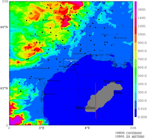
This first simulation was made at a horizontal resolution of 1 km over an area covering about 50 000 km², and centred on the Thau lagoon, the surface of which does not exceed 80 km². For that reason, and also in order to study the interaction between the breeze and the lagoon, it was necessary to define a model with higher horizontal resolution. The 6 UTC output of the initial simulation was used to initialise the next 12-hour model forecast, based on a two-way grid nesting method (Stein et al., 2000), involving two nested models of 1-km and 200-m horizontal resolution exchanging the state variables at each time step. The two integration domains are presented in Fig. 8. A one-dimensional turbulent scheme based on Bougeault and Lacarrère (1989) is used in the 1-km model whereas a three-dimensional turbulent scheme is activated in the 200-m model, based on the Deardorff (1980) approach. Both models share the same shallow convection scheme, based on the eddy mass flux approach (Soares, 2004; Pergaud et al., 2009). The vertical grid was defined such that the lower layers are well represented: there are about 20 levels below 1000 m and the ground, and 10 levels below 300 m. The analysis from the French operational AROME model (Seity et al., 2011) is used every 3 hours as large-scale atmospheric coupling and to initialise the upper air and surface variables. This model configuration is hereafter referred to as MFLK (for Model and FLake).

Fig. 8 Simulation domains located in the south of France at the Mediterranean Sea. The bigger domain shows the orography of the area, with the Mediterranean coastline (black line) and the lake contours (thin black line), whereas the limits of the 200-m resolution domain are represented in a square, zoomed on the bottom-right part of the figure, in which the north–south oriented red line represents the axis of the vertical cross-section. Black dots correspond to the stations of the French observation network (only a few names are indicated).

3.2.2. Numerical experiments.

The first step was aimed at verifying that the Thau lagoon was well represented at a resolution of 200 m. Indeed, the ECOCLIMAP land-use database (Masson et al., 2003) has a nominal resolution of 1 km. At this scale, the strip of land separating the lagoon from the Mediterranean Sea, known as the Lido, which is only 1-km wide and 12-km long, was not represented. It was therefore necessary to add a strip of land to represent this limit. An ecosystem representative of the surrounding vegetation was added, composed of 63% sand and 21% grassland. The associated orography was calculated from the SRTM (Shuttle Radar Topography Mission) 90-m digital elevation database (http://www.cgiar-csi.org/data/srtm-90m-digital-elevation-database-v4-1). Over the past decade, significant efforts have helped to consolidate the Lido and ensure protection against erosion. This strip of land is vital to the survival of thousands of jobs based around the lagoon. A second experiment referred to as MNLD (Model NoLanD) was carried out with the same numerical configuration, initialisation and forcing, with the strip of land removed and the orography suppressed. The MNLD experiment was compared to MFLK, the most realistic experiment in terms of land cover and orography. This comparison is discussed in Section 4.2.5. To evaluate the benefit of representing the diurnal cycle of the lake surface temperature, another simulation referred to as MWAT was created with the same model configuration as MFLK but with the FLake model turned off and the surface temperature kept constant during the model run. The comparison with MFLK is described in Section 4.2.2.

4. Model results and discussion

4.1. Off-line simulations

4.1.1. Calibration of the extinction coefficient.

The FLake model was first used in standalone mode, forced by the observations made at the Marseillan table over the THAUMEX period between 6 August and 6 October. The first requirement was to determine as precisely as possible, the extinction coefficient of the lagoon, denoted as k in eq. 5.

Potes et al. (2012) have shown that the model was sensitive to the light extinction coefficient. Because of the shallowness of the Thau lagoon, the attenuation of light plays an even more important role in the energy balance of the water column. Compared with deeper lakes such as Alqueva (Lindim et al., 2011) in Portugal (16.6 m average and 96 m maximum) or Ladoga (Sorokin et al., 1996) in Russia (51-m average), where the FLake model is essentially sensitive to the depth (Salgado and Le Moigne, 2010; Balsamo et al., 2010), in Thau, the model has a higher sensitivity to light extinction. An increase of the extinction coefficient of 0.05 m⁻¹ leads to a warming of 0.2°C at the Marseillan table. The result was that for FP1, for a depth of 4 m, the extinction coefficient that minimised the RMSE between the observed and simulated temperature was k=0.48 m⁻¹. This was valid for all time windows of minimisation, and all periods of recovery considered. Figure 2e also shows the simulated surface temperature (OFLK) as a function of time. The result is quite satisfactory when compared to the near-surface observed temperature, since the bias between the two series is −0.03°C, with a standard deviation of 0.29°C. Both series are highly correlated with a correlation R=0.95. However, the model tends to underestimate the magnitude of the observed daily temperature amplitude. Indeed, during the night, the model is a bit warmer than reality, while during the day it slightly underestimates the maximum temperature. In FP2, the result is a little different, since whatever the considered minimisation window and recovery periods, the frequency diagrams are bimodal. Indeed, the two coefficients k=0.23 and 0.31 have a higher frequency of occurrence than others and minimise the error in the case of the parameterisation FP2. The two simulations, performed with these coefficients, have a mean bias of −0.37°C (standard deviation 0.55°C) and 0.32°C (standard deviation 0.51°C), respectively. FP1 parameterisation, leading to better results for the surface temperature, will be used later in the study. The calibrated extinction coefficient (0.48 m⁻¹) is well within the range found from radiance measurements that have a mean value of 0.52 m⁻¹ (see Section 2.4.5).

The same depth and extinction (FP1) settings were tested on a completely independent data set, covering the period from December 2008 to December 2010. The statistical results for the surface temperature show a mean bias of 0.36°C with a standard deviation of 0.46°C. The results of this 2-yr-long experiment show that the extinction coefficient for the THAUMEX period can be used as a parameter of the FLake model for the Thau lagoon.

4.1.2. Energy budget components

4.1.2.1. Surface fluxes. Time series of sensible and latent heat fluxes were then compared with model results. The hourly mean values of the latent heat flux QE are always significantly higher than the hourly mean values of the sensible heat flux QH, showing that the turbulent heat exchanges are dominated by evaporation. The comparison with observations revealed a weak negative bias of −1.9 W m⁻² (12.3 W m⁻² standard deviation) for QH as shown in Fig. 9b, and a rather high overestimation of 28.7 W m⁻² on average (58.1 W m⁻² standard deviation) for QE as indicated in Fig. 9a. The satisfactory results of QH are directly related to the accuracy of the surface temperature, since it depends on the vertical temperature gradient between the surface and the measurement height. These results are confirmed by the modelled daily cycles of QH, QE and surface temperature as illustrated in Fig. 10.

Fig. 9 IOP2 scatter plot (a) of latent heat flux (QE) for observations (OBS) and model (OFLK) during the day (black dots) and night (red dots); scatter plot (b) of sensible heat flux (QH) for observations (OBS) and model (OFLK) during the day (black dots) and night (red dots).

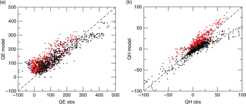
Fig. 10 Average daily cycle for observations (OBS) and model (OFLK), of surface temperature (a) and surface latent and sensible heat fluxes (b).

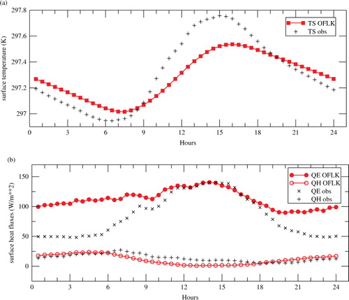
Conversely, the excessive evaporation is particularly intense at night. The bias calculated between 21 UTC and 3 UTC is 49.8 W m⁻² (38.1 W m⁻² standard deviation) while it is only 6.5 W m⁻² (48.8 W m⁻² standard deviation) during the day, between 9 UTC and 15 UTC. Among the numerous studies, only a few have examined in detail the distribution of evaporation between night and day. Salgado and Le Moigne (2010) have analysed the evaporation at local scale based on a daily cycle, whereas Dutra et al. (2010) have examined global-scale averages of the energy budget components, and particularly evaporation. The dependence of model surface fluxes on wind and temperature or humidity gradient was examined and the correlation coefficient computed for the 2-month period. As previously mentioned, a high correlation (R=0.84) exists between QH and the temperature gradient, and also between QE and the specific humidity gradient (R=0.68). The evaporation flux is however strongly correlated (R=0.76) to wind speed. The low correlation (R=0.19) between the sensible heat flux QH and the wind speed U can be explained by the air stability above the water. During the THAUMEX period, a wind speed increase is usually associated with air cooling, the result of either the cold tramontana from the north or sea breezes from the south. In both cases, a cold air advection is experienced at the coast. The decrease of the temperature gradient inhibits the effect of the wind speed increase on the sensible heat flux. High correlations (0.96, 0.94) exist by construction between (QH, QE) and (U(T _s –T _a ), U(q _s –q _a )), respectively. Bouin et al., (2012a) have used an aerodynamic method to calculate the surface turbulent fluxes, which is similar to our model formulation, and have obtained correlations of (0.96, 0.78). However, such correlations calculated on EC measurements (Blanken et al., 2000; Blanken et al., 2003; Nordbo et al., 2011) have shown that the latent heat flux was better explained by U(q _s –q _a ) and the sensible heat flux by U(T _s –T _a ), which corroborates the model results.

In addition to QH and QE, the momentum flux QM, reflecting the surface stress at the water surface was evaluated. More precisely, we compared the modelled (bulk formulation) and observed friction velocities defined as , where ρ _air is the air density close to the surface. The average friction velocities are comparable over the THAUMEX period; however, the model exhibits a lower friction. The mean u _* bias between the model and the EC measurements is 0.047 m s⁻¹ with an RMSE of 0.07 m s⁻¹ for an averaged u _* close to 0.2 m s⁻¹ in both cases, with no significant distinction between night and day.

4.1.2.2. Energy budget. The energy budget equation (4) was applied to the observations in order to estimate the heat flux QB exchanged with the sediment layer; therefore, QB was solved as a residual of the energy balance. But, most of the time, the energy balance closure is not ensured by EC flux measurements (Nordbo et al., 2011): some of the largest eddies can be missed by measurements and uncertainties on EC footprints, that depend on air stability or wind, can affect the closure, leading to a flux underestimation. However QN and the water temperature measurements used to compute QW are also sources of errors. Consequently, a systematic error due to measurements is made on QB. As far as the observations are concerned, <T> was computed according to eq. (1) applied to the temperature profile measurements and ∂ < T>/∂t was estimated by a first-order Taylor development, which approximates the derivative of <T> by its growth rate between two consecutive instants. The sediment module was not activated in the model due to a lack of temperature measurement in the sediment layer needed for flux computations. So in the model, QB was zero and eq. (4) was then used to estimate QW from model output. This approach was preferred to that used for the observations, in order not to introduce model error on the mean temperature profile on the one hand and on its time derivative on the other hand. The two computing methods of QW led to an absolute maximum difference of 10 W m⁻² over the whole THAUMEX period. Table 3 summarises the observed (OBS) and modelled (OFLK) components of the water energy budget for the THAUMEX period. As expected, net radiation appears similar in the observations and the model; in both cases the net solar radiation is the same and the difference lies only in the surface temperature. Radiative measurements involve a radiative surface temperature reacting as a skin temperature, whereas the model surface temperature is representative of a water thickness ranging from a few centimetres to several metres. Sensible heat fluxes are also very close. The model evaporation is overestimated by 26 W m⁻², particularly at night, when it is almost doubled. During the THAUMEX period, the lagoon releases heat: 4 W m⁻² for OBS and 12 W m⁻² for OFLK. However, excessive heat release is experienced due to the nighttime evaporation combined with the heat loss caused by the radiative surface cooling. In OBS, the net surface radiation (141 W m⁻²) is in balance with the surface turbulent heat fluxes (95 W m⁻²), combined with the portion solar heat that reaches the bottom (29 W m⁻²) and the heat content of the water (−4 W m⁻²), leading to a positive flux from the water to the sediment layer (21 W m⁻²). Contrarily, in OFLK, a higher surface temperature (0.15 K on average) leads to lower QN (135 W m⁻²) which, combined with an overestimated turbulent heat flux (23 W m⁻²), leads to a stronger heat release from the water column because no energy is exchanged with the sediment layer. The large evaporation observed at night in OFLK (42 W m⁻²) is split almost equally in OBS between evaporation (+23 W m⁻²) and storage of heat in the sediments (+25 W m⁻²).

Table 3. Energy budget components (W m⁻²) averaged over the whole period for the observations (OBS), the model (OFLK) and the experiment where surface temperature derived from radiation measurements is used instead of model surface temperature (DIAG)

QN	I(D)	QW	QE	QH	QB
Day	OBS	171	29	84	57	7	−6
OFLK	167	29	70	63	3	0
DIAG	171	29	84	58	2	−2
Night	OBS	−29	0	−84	23	7	25
OFLK	−31	0	−80	42	7	0
DIAG	−29	0	−84	33	3	19
Total	OBS	141	29	−4	82	13	21
OFLK	135	29	−12	108	10	0
DIAG	141	29	−4	93	5	18

4.1.2.3. Model surface fluxes computed from a radiative temperature. Next, we attempted to diagnose the surface fluxes by using a bulk formulation as in eqs. (7) and (8), but where the model surface temperature was replaced by the surface radiative temperature derived from the radiation observations and computed by eq. (2). These are the fluxes that the model would be able to compute if it could distinguish a skin temperature from the mixed layer temperature of the lagoon. We recomputed the surface-specific humidity at saturation, kept the model exchange coefficients for heat and vapour aligned with the model temperature and updated the net radiation in order, ultimately, to diagnose the components of the energy budget (column DIAG of Table 3). Unsurprisingly, diagnosed net radiation fits the observed net radiation, QH is lower than in OBS by 8 W m⁻², and the 32% overestimation of QE is reduced to 13%, proving that part of the overestimation of QE in the model is due to its relative inability to simulate the radiative nighttime cooling accurately. In such a configuration, the total amount of turbulent heat flux differs from the observations by only 1 W m⁻², although the Bowen ratio is three times higher in DIAG than in OBS, and the bottom flux (18 W m⁻²) approaches the one computed from measurements (21 W m⁻²). During the day, the bottom flux QB is always low and negative, showing that the sediment layer supplies energy to the water (6 W m⁻² for OBS and 2 W m⁻² for DIAG), as during daytime the solar radiation heats the bottom layer which then transfers part of this energy to the water via direct sensible heat flux. On the contrary, at night, the sediment layer acts as a sink and extracts energy from the water by about 25 W m⁻² for OBS.

4.1.3. Mixed layer depth.

In the model, when the mixed layer does not reach the bottom, the depth of the thermocline – the region between the mixed layer and the bottom – is a good indicator of stratification. However, to assess the model's ability to reproduce the stratification of the water column, we used δT=T _s –T _b , the temperature difference between surface (T_s ) and bottom (T_b ). A positive δT during summer reflects the presence of a mixed layer near the surface, whereas when δT is close to zero, the mixing is nearly complete. Figure 11a shows the time evolution of δT for the model and the observations over the THAUMEX period. The first remark is that the model tends to be thoroughly mixed, while observations indicate that a stratification exists almost all the time (the observed vertical gradient is nonzero). It is not typical for FLake to predict a thoroughly mixed water column. The LakeMIP intercomparison exercise (Stepanenko et al., 2010) has shown that during summer time, the FLake model exhibited a realistic stratification. However, shallow lakes can be totally mixed all the time, like Balaton Lake for instance (Vörös et al., 2010) or only in summer due essentially to wind conditions that mix the water from top to bottom (Kirillin, 2003). In the model, δT is lower than in the observations. The difficulty of the model to represent the stratification accurately may be related to the shallowness of the lagoon, which in addition has a low extinction coefficient, promoting the penetration of solar irradiance to the bottom. The second reason relates to the simplicity of the model, which accounts for only two layers and promotes rapid energy exchanges between surface and bottom. This also explains why the bottom temperature is often very similar to the surface temperature. Figure 11b represents T_s and T_b for the model and the observations, for a 4-d period where the model exhibits a stratification. In this particular case, the model manages to keep the stratification over 3 d, but with a lower amplitude than what is observed. However, the model bottom temperature highlights a strong increase at night, making the whole water column homogeneous. In the late afternoon, the surface temperature decreases while the mixed layer thickens and the colder water sinks; therefore, the mean water temperature also decreases. Furthermore, the water column gradually homogenises, whereas the bottom temperature increases. When the mixed layer depth is equal to the total lagoon depth, the bottom temperature undergoes a relatively rapid increase to equal the surface temperature, which reflects a full mixing.

Fig. 11 (a) Time evolution of the difference between surface (T _s ) and bottom temperature (T _b ) in the model (OFLK) and the observations (OBS), (b) modelled (solid red) and observed (T _s ) (solid black), modelled (dashed red) and observed (T _b ) (dashed black) over a 4-d stratified period.

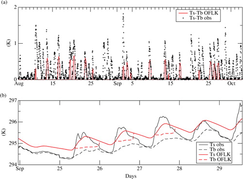
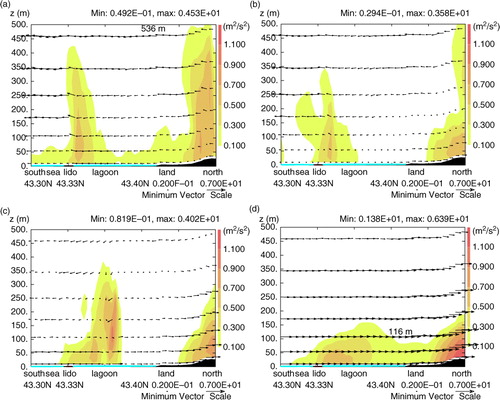
Fig. 12 Vertical cross-section of TKE superimposed onto wind during IOP2. (a), (b), (c) and (d) correspond respectively to 09, 10, 11 and 12 UTC. Numbers on (a) and (d) correspond to the observed ABL height.

4.2. MFLK-coupled simulations

4.2.1. ABL height.

We then calculated the height of the boundary layer in order to quantify the previous results. Table 4 shows the values of the boundary layer height calculated in this way for each radio-sounding, for experiments MFLK and MNLD. Despite the small number of ABL observations, it seems that the transition to the sea breeze is better represented in the MFLK experiment than in the MNLD one, where turbulence is more developed due to the presence of the Lido, which enhances friction and tends to warm up more, and more quickly, than water.

Table 4. Boundary layer height (m) measured and modelled at 09 UTC, 12 UTC and 15 UTC

09 UTC	12 UTC	15 UTC
Observations	536	116	103
MFLK	399	79	107
MNLD	295	107	107

Such a transition from land breeze to local morning breeze, evolving afterwards to a regional breeze in the afternoon, was already observed and modelled (Puygrenier, 2005) during the ESCOMPTE field campaign near Marseille, in southern France. The MFLK experiment showed the same characteristics. Figure 12a–d shows a cross-section (axis shown on Fig. 8) from south to north of the turbulent kinetic energy (TKE hereafter) superimposed on the wind at times 09, 10, 11 and 12 UTC, respectively. As mentioned previously, at 09 UTC, the land breeze was widespread in the model in the region of interest. An hour later, a local southern breeze began between the lagoon and the land in the northern part of the domain, while a north wind component was still evident from the Lido to the Mediterranean Sea. The displacement of the breeze front on the continent was associated with a return current to the rear, and generated subsidence at approximately 400 m over the lagoon. This downdraft induced divergence at the surface and fed both the local breeze generated by the lagoon and the residual land breeze (Fig. 12b). An hour later (Fig. 12c), the local breeze intensified due to the warming of the continent, causing a more intensive updraft and reinforcing the return current. At the same time, the regional sea breeze reached the Lido, advecting the Lido turbulent cell to the lagoon, intensifying it and creating a secondary breeze front characterised by ascending and subsiding air motions (Fig. 12c). The regional breeze was generalised at 12 UTC and superimposed to the local breeze regimes, which then disappeared. Consequently, the boundary layer height dropped below 100 m over the lagoon and below 400 m over land.

4.2.2. Validation over land.

Another validation of the three-dimensional simulation was realised over land. The goal was to evaluate the accuracy of the model by making comparisons with air temperature and relative humidity at 2 m, and wind at 10 m. Table 5 returns the 3-hour average bias and RMSE, computed over the 90 stations, between 06 UTC and 18 UTC, for these surface variables. It highlights the good model results, as biases of all variables are smaller than the accuracy of the instruments (Table 1) and, furthermore, RMSEs are relatively low.

Table 5. IOP2 3-hourly averaged biases and RMSEs computed from 90 meteorological stations over land between 06 UTC and 18 UTC for 2 m temperature, relative humidity and the components of 10 m wind, using MFLK model configuration

T2M (C)	HU2M (%)	U10M (m s^−1)	V10M (m s^−1)
Mean bias	−0.14	1.12	−0.38	−0.32
Mean RMSE	2.26	11.76	2.26	2.74

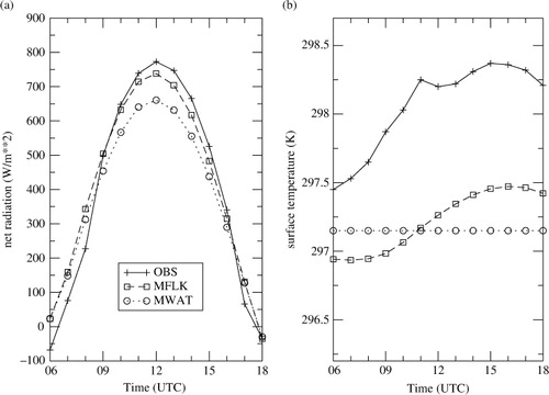
Another model configuration (MWAT) was tested, in order to evaluate the impact of the use of FLake model. The MWAT experiment was derived from the MFLK model configuration but with the FLake model turned off. In the MWAT experiment, the lake surface temperature was kept constant during the run and surface fluxes were computed using the Louis formulation; this model configuration is currently used operationally in French mesoscale forecast models. The results in terms of average biases and RMSEs over the whole domain are very close to those obtained with MFLK, indicating that the regional-scale air circulation was not affected by the lake parameterisation itself, as expected given the small surface area covered by the lagoon. However, when FLake is activated, the local energy balance computed over the lagoon is improved for two reasons. First, the albedo dependence on the zenith angle significantly improves the net radiation computation as shown in Fig. 13a, where the relative error at noon calculated at the Marseillan station is 4% when FLake and its albedo are used, as compared with 15% for the MWAT configuration, in which the albedo is 0.135. In the early morning, both model configurations are less sensitive to the albedo and overestimate the net radiation due to the presence of low clouds advected by the land breeze. Second, the time evolution of the surface temperature is well reproduced with MFLK, as shown in Fig. 13b, even if a cold bias is experienced by the MFLK model. However, the objective of a comparison between in situ observations and the model forecast is to verify that the model behaves correctly, especially as the observations were not assimilated through a data assimilation process.

Fig. 13 Net radiation (a) and surface temperature (b) observed (solid line with crosses), modelled by MFLK (dashed line with squares) and by MWAT (dotted line with circles), for IOP2.

4.2.3. Surface fluxes.

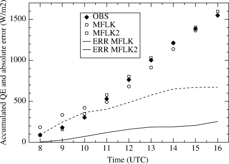
We then tried to evaluate the lake model's ability to represent surface fluxes during IOP2. When comparing the time evolution of the modelled surface fluxes with the measured ones, it turned out that the evaporation QE exhibited a good consistency of the daily evolution in shape and amplitude. However, as previously mentioned, the model sea-breeze establishment was late by approximately 2 hours. When the model result is shifted by 2 hours to simulate an on-time breeze forecast, the accumulated error on the evaporative flux is largely reduced compared to the initial run. Figure 14 shows the accumulated latent heat flux (symbols) for the observations (OBS), the model (MFLK) and the 2-hour shifted model (MFLK2), as well as the accumulated absolute error for the model (ERR MFLK) and the 2-hour shifted model (ERR MFLK2), and demonstrates that the error is reduced by about 400 W m⁻² when shifting is applied. Modelled and measured sensible heat fluxes QH do not reflect such a marked daily cycle because surface temperature does not exhibit a large thermal amplitude and therefore does not evolve rapidly during the day. This comparison proves that the model computations of the surface heat fluxes QH and QE are reliable.

Fig. 14 Time evolution of accumulated latent heat flux QE (symbols) and associated absolute error for the model (ERR MFLK) and the 2-hour shifted model (ERR MFLK2).

4.2.4. Sensitivity to the Lido.

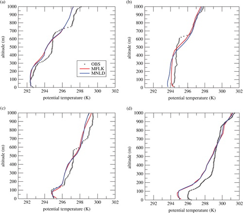
The two experiments MFLK and MNLD were compared with radio-soundings launched from the Marseillan platform, to assess the influence of the Lido on the structure of the lower layers of the atmosphere. According to the observations, at 07 UTC, a land breeze was still sensitive on the lagoon. Then, during the morning, around 08:30 UTC, the sea breeze started up and strengthened gradually during the late morning and the afternoon. The model, meanwhile, retained a north wind until approximately 11 UTC, reflecting the persistence of the land breeze. At 07 UTC, the observed vertical profile of potential temperature (Fig. 15) showed strong gradients, smoothed by the model. Moreover, both experiments showed a colder temperature profile (about 0.5°C) in the first kilometre of the atmosphere, as compared to the observation, indicating that the model nighttime cooling was probably too strong. However, in the lower layers, the profiles are similar and show a first mixed layer, up to about 250 m, caused by the shear induced by the land breeze. A residual layer, reflecting the past convection, was 700 m high according to the observations and only 600 m in the model. At 09 UTC, the presence of natural vegetation near the sea/lagoon interface generated more turbulence in MFLK experiment, especially because of a higher roughness length and a lower heat capacity. As a consequence, the height of the boundary layer was lower in the MNLD experiment. In addition, weaker vertical mixing was detected in MNLD, leading to colder temperatures near the surface and the first atmospheric layers (Fig. 15). At this time, the MFLK profile is closer to the observed one. Subsequently, when the transition was made between the land breeze regime, the calm period that followed and the establishment of the sea breeze, the sea breeze strengthened and the height of the boundary layer abruptly decreased, highlighting a stratification that did not exceed 100 m. At 12 UTC, with the sea breeze already established, the temperature, humidity and wind profiles were quite similar in the observations in both experiments. Later, at 15 UTC, the profiles were also very similar, but the model showed a tendency to generate too strong a breeze, and therefore a slightly underestimated temperature in the boundary layer.

Fig. 15 Potential temperature profiles at 07, 09, 12 and 15 UTC. The crosses is radio-sounding, red line corresponds to MFLK and blue to the MNLD experiment.

5. Conclusion

Over the course of this study, we were able to collect not only standard meteorological data but also EC fluxes, which are necessary for evaluating the parameterisation of the FLake model surface fluxes. Additionally, we developed a special device to measure the temperature profile of the lagoon at the Marseillan station, as these data are essential to the validation of the model. Second, we examined the coupling between Meso-NH and FLake via SURFEX. We have shown that the coupling was working properly. This was the first time a three-dimensional coupled run with Meso-NH model was performed using FLake and compared to existing observations. Despite the time lag observed during the breeze episode, which was mainly due to the fact that the dynamics of the model that day did not accurately reproduce reality, the surface fluxes and consequently the surface temperature were correctly reproduced by the coupled system. This confirms that the fluxes are correctly computed by the FLake model, which underlines the fact that the latent heat flux was dominating the sensible heat flux. This result was also obtained in off-line mode, as we were able to compute an energy budget for the whole water column and estimate the role of the sediment layer. While it acts as an energy sink at night, it is an energy source during the day. We highlighted the sensitivity to the light extinction coefficient and were able to calibrate it to obtain the best surface temperature, the key variable in the coupling process. It turned out that the model was very sensitive to the extinction coefficient of the lake in this particular study, which has involved a clear and shallow water body. We also highlighted the difficulty involved in using the model to retrieve the surface temperature computed from satellite measurements, but were able to explain some of the discrepancies in the surface fluxes by analysing the differences between the radiative temperature and the model bulk one. Local studies such as this are of great importance for validating our models and analysing the parameterisations that compose them. The complementarities between the ‘off-line’ and the ‘on-line’ runs allowed the validation of the Meso-NH/FLake coupling at mesoscale.

Acknowledgements

The authors are very grateful to the people who initiated this work on the Thau lagoon, particularly J. Noilhan, whose enthusiasm was always a source of motivation. They thank S. Faroux for providing the land-use map for the experiment without Lido. The discussions with G. Caniaux and G. Pigeon during the analysis of the lagoon water budget and the surface energy budget, respectively, were very helpful.

References

- Balsamo G , Dutra E , Stepanenko V. M , Viterbo P , Miranda P. M. A , Mironov D . Deriving an effective lake depth from satellite lake surface temperature data: a feasibility study with MODIS data. Boreal Environ. Res. 2010; 15: 178–190.
- Balsamo G , Salgado R , Dutra E , Boussetta S , Stockdale T , Potes M . On the contribution of lakes in predicting near-surface temperature in a global weather forecasting model. Tellus A. 2012; 64(2012): 15829.
- Banas D , Grillas P , Auby I , Lescuyer F , Coulet E , co-authors . Short time scale changes in underwater irradiance in a wind-exposed lagoon (Vaccares lagoon, France): efficiency of infrequent field measurements of water turbidity or weather data to predict irradiance in the water column. Hydrobiologia. 2005; 551(1): 3–16.
- Bessemoulin P . Méthodes expérimentales de détermination des flux de surface (Experimental methods for determining the surface fluxes). 1993. Technical report, Note de centre GMME n6. Centre National de Recherches Météorologiques.
- Blanken P. D , Rouse W. R , Culf A. D , Spence C , Boudreau L. D , co-authors . Eddy covariance measurements of evaporation from Great Slave Lake, Northwest Territories, Canada. Water Resour. Res. 2000; 36(4): 1069–1077.
- Blanken P. D , Rouse W. R , Schertzer W. M . Enhancement of evaporation from a large northern lake by the entrainment of warm, dry air. J. Hydrometeorol. 2003; 4(4): 680–693.
- Bougeault P , Lacarrère P . Parameterization of orography-induced turbulence in a meso-beta scale model. Mon. Weather Rev. 1989; 117: 1870–1888.
- Bouin M.-N , Caniaux G , Traullé O , Legain D , Le Moigne P . Long-term heat exchanges over a Mediterranean lagoon. J. Geophys. Res. 2012a; 117: 23104.
- Bouin M.-N , Legain D , Traulle O , Belamari S , Caniaux G , co-authors . Using scintillometry to estimate sensible heat fluxes over water: first insights. Boundary-Layer Meteorol. 2012b; 143(3): 451–480.
- Boyle J. P . Field results from a second-generation ocean/lake surface contact heat flux, solar irradiance, and temperature measurement instrument – the multisensor float. J. Atmos. Ocean. Tech. 2007; 24: 856–876.
- Canut G , Couvreux F , Lothon M , Pino D , Said F . Observations and large eddy simulation of entrainment in the sheared Sahelian boundary layer. Boundary-Layer Meteorol. 2012; 142(1): 79–101.
- Deardorff J.-W . Stratocumulus-capped mixing layers derived from a three-dimensional model. Boundary-Layer Meteorol. 1980; 18: 495–527.
- Derolez V , Soudant D , Fiandrino A , Cesmat L , Serais O . Impact of weather conditions on Escherichia coli accumulation in oysters of the Thau lagoon (the Mediterranean, France). J. Appl. Microbiol. 2013; 114(2): 516–525.
- Dutra E , Stepanenko V. M , Balsamo G , Viterbo P , Miranda P. M. A , co-authors . An offline study of the impact of lakes on the performance of the ECMWF surface scheme. Boreal Env. Res. 2010; 15: 100–112.
- Finch J , Calver A . Methods for the Quantification of Evaporation from Lakes. 2008; Prepared for the World Meteorological Organization Commission of Hydrology, CEH Wallingford, UK.
- Flocas H. A , Kelesis A , Helmis C. G , Petrakakis M , Zoumakis N . Synoptic and local scale atmospheric circulation associated with air pollution episodes in an urban Mediterranean region. Theor. Appl. Climatol. 2009; 95: 265–277.
- Fritz J. J , Meredith D. D , Middleton A. C . Non-steady state bulk temperature determination for stabilization ponds. Water Res. 1980; 14: 413–420.
- Garrett A , Kurzeje R , O'steen B , Parker M , Pendergast M , co-authors . Observations and model predictions of water skin temperatures at MTI core site lakes and reservoirs. Proc. SPIE – The International Society for Optical Engineering. 2001; 4381: 225–235.
- Harris L , Rao Kotamarthi V . The characteristics of the Chicago Lake breeze and its effects on trace particle transport: results from an episodic event simulation. J. Appl. Meteorol. 2005; 44: 1637–1654.
- Hook S.-J , Prata F , Alley R. E , Abtahi A , Richards R. C , co-authors . Retrieval of lake bulk and skin temperatures using Along-Track Scanning Radiometer (ATSR-2) data: a case study using Lake Tahoe, California. J. Atmos. Ocean. Tech. 2003; 20: 534–548.
- Hostetler S.W , Giorgi F , Bates G.T , Bartlein P.J . Lake-Atmosphere Feedbacks Associated with Paleolakes Bonneville and Lahontan. Science, New Series. 1994; Vol 263., No. 5147, American Association for the Advancement of Science. 665–668.
- Kanakidou M , Mihalopoulos N , Kindap T , Im U , Vrekoussis M , co-authors . Megacities as hot spots of air pollution in the East Mediterranean. Atmos. Environ. 2011; 45(6)
- Kheyrollah Pour H , Duguay C , Martynov A , Brown L. C . Simulation of surface temperature and ice cover of large northern lakes with 1-D models: a comparison with MODIS satellite data and in situ measurements. Tellus A. 2012; 64: 17614.
- Kirillin G , Terzhevik A. Y . Modelling of the shallow lake response to climate variability. Proceedings of the 7th Workshop on Physical Processes in Natural Waters. 2003; Northern Water Problems Institute of the Russian Academy of Sciences, Petrozavodsk, Karelia, Russia. 144–148.
- Kjerfve B . Coastal Lagoon Processes, Elsevier Oceanography Series. 1994; Vol 60, Elsevier, Amsterdam. 69–101.
- Kourzeneva E . External data for lake parameterization in Numerical Weather Prediction and climate modeling. Boreal Environ. Res. 2010; 15: 165–177.
- Kourzeneva E , Braslavsky D , Undèn P . Lake model FLake, coupling with atmospheric model: first steps. Fourth SRNWP/HIRLAM Workshop on Surface Processes and Assimilation of Surface Variables jointly with HIRLAM Workshop on Turbulence, Workshop report. 2005; SMHI, Norrköping, Sweden. 43–53.
- Krinner G . Impact of lakes and wetlands on boreal climate. J. Geophys. Res. 2003; 108(D16): issn: 0148–0227. ACL 10-1 to ACL 10-18.
- Lafore J. P , Stein J , Asencio N , Bougeault P , Ducrocq V , co-authors . The Meso-NH atmospheric simulation system. Part I: adiabatic formulation and control simulations. Ann. Geophys. 1998; 16: 90–109.
- Lehner B , Döll P . Development and validation of a global database of lakes, reservoirs and wetlands. J. Hydrol. 2004; 296(1–4): 1–22.
- Le Moigne P , Boone A , Decharme B , Faroux S , Gibelin A.-L , co-authors . Surfex Scientific Documentation. 2009. Technical Report, Centre National de Recherches Météorologiques, Toulouse.
- Lindim C , Pinho J. L , Vieira J. M. P . Analysis of spatial and temporal patterns in a large reservoir using water quality and hydrodynamic modeling. Ecol. Model. 2011; 222: 2485–2494.
- Lothon M , Couvreux F , Durand P , Hartogensis O.K , Legain D . The boundary-layer late afternoon and sunset turbulence field experiment. Proceedings of the 20th Symposium on Boundary-Layers and Turbulence. 2012; American Meteorological Society, Boston, MA. pp. 14B.1: July. 9–13.
- Louis J.-F . A parametric model of vertical eddy fluxes in the atmosphere. Boundary-Layer Meteorol. 1979; 17: 187–202.
- Mascart P , Noilhan J , Giordani H . A modified parameterization of flux-profile relationships in the surface layer using different roughness length values for heat and momentum. Boundary-Layer Meteorol. 1995; 72: 331–344.
- Masson V , Champeaux J.-L , Chauvin F , Meriguet C , Lacaze R . A global data base of land surface parameters at 1 km resolution in meteorological and climate models. J. Clim. 2003; 16: 1261–1282.
- Mironov D. V , Zilitinkevich S. S . Air–water interaction parameters over lakes. Modeling Air–Lake Interaction. Physical Background. 1991; Springer-Verlag, Berlin. 50–62.
- Mironov D. V . Parameterization of lakes in numerical weather prediction. Description of a lake model. 2008; COSMO Technical Report, No. 11, Deutscher Wetterdienst, Offenbach am Main, Germany. 41.
- Monin A. S , Obukhov A. M . Basic laws of turbulent mixing in the surface layer of the atmosphere. Tr. Akad. Nauk SSSR Geofiz. Inst. 1954; 24: 163–187.
- Noilhan J , Donier S , Lacarrere P , Sarrat C , Le Moigne P . Regional-scale evaluation of a land surface scheme from atmospheric boundary layer observations. J. Geophys. Res. 2011; 116: 01104.
- Nordbo A , Launiainen S , Mammarella I , Leppäranta M , Huotari J , co authors . Long-term energy flux measurements and energy balance over a small boreal lake using eddy covariance technique. J. Geophys. Res. 2011; 116: D02119.
- Perez-Ruzafa A . Detecting changes resulting from human pressure in a naturally quick-changing and heterogeneous environment: Spatial and temporal scales of variability in coastal lagoons. Estuar. Coast. Shelf Sci. 2007; 75: 175–188.
- Pergaud J , Masson V , Malardel S , Couvreux F . A parameterization of dry thermals and shallow cumuli for mesoscale numerical weather prediction. Boundary-Layer Meteorol. 2009; 132(1): 83–106.
- Potes M , Costa M. J , Salgado R . Satellite remote sensing of water turbidity in Alqueva reservoir and implications on lake modelling. Hydrol. Earth Syst. Sci. 2012; 16: 1623–1633.
- Potes M , Costa M. J , Salgado R , Bortoli D , Serafim A , co-authors . Spectral measurements of underwater downwelling radiance of inland water bodies. Tellus A. 2013; 65
- Potes M , Costa M. J , Silva J. C. B , Silva A. M , Morais M . Remote sensing of water quality parameters over Alqueva reservoir in the south of Portugal. Int. J. Remote Sens. 2011; 32(12): 3373–3388.
- Puygrenier V , Lohou F , Campistron B , Saïd F , Pigeon G , co-authors . Investigation on the fine structure of sea-breeze during ESCOMPTE experiment. Atmos. Res. 2005; 74: 329–353.
- Salgado R , Le Moigne P . Coupling of the FLake model to the Surfex externalized surface model. Boreal Environ. Res. 2010; 15: 231–244.
- Samuelsson P , Kourzeneva E , Mironov D . The impact of lakes on the European climate as simulated by a regional climate model. Boreal Env. Res. 2010; 15: 113–129.
- Schneider P , Hook S. J . Space observations of inland water bodies show rapid surface warming since 1985. Geophys. Res. Lett. 2010; 37: 22405.
- Seity Y , Brousseau P , Malardel S , Hello G , Bénard P , co-authors . The AROME-France Convective-Scale operational model. Mon. Weather Rev. 2011; 139: 976–991.
- Smith N. P , Kjerfve B . Chapter 4 water, salt and heat balance of coastal lagoons. Elsevier Oceanography Series. 1994; 60 Elsevier, Amsterdam. 69–101. ISSN 0422-9894, ISBN 9780444882585, 10.1016/S0422-9894(08)70009-6.
- Smith R. C , Baker K. S . Optical properties of the clearest natural waters (200–800 nm). Appl. Opt. 1981; 20: 177–184.
- Soares P.-M , Miranda P. M. A , Siebesma A. P , Teixeira J . An eddy-diffusivity/mass-flux parameterization for dry and shallow cumulus convection. Q. J. Roy. Meteorol. Soc. 2004; 130: 3365–3384.
- Sorokin A. I , Naumenko M. A , Veselova M. F . New morphometrical data of Lake Ladoga. Hydrobiologia. 1996; 322(1–3): 65–67.
- Stein J , Richard E , Lafore J.-P , Pinty J.-P , Asencio N , co-authors . High-resolution non-hydrostatic simulations of flash-flood episodes with grid-nesting and ice-phase parametrization. Meteorol. Atmos. Phys. 2000; 72: 101–110.
- Stepanenko V. M , Goyette S , Martynov A , Perroud M , Fang X , co-authors . First steps of a Lake Model Intercomparison Project: LakeMIP. Boreal Environ. Res. 2010; 15: 191–202.
- Taylor J. P , Edwards J. M , Glew M.-D , Hignett P , Slingo A . Studies with a flexible new radiation code. II: comparisons with aircraft shortwave observations. Q. J. Roy. Meteorol. Soc. 1996; 122: 839–861.
- Vörös M , Istvánovics V , Weidinger T . Applicability of the FLake model to Lake Balaton. Boreal Environ. Res. 2010; 15: 245–254.