Comparison of non-homogeneous regression models for probabilistic wind speed forecasting

Abstract

In weather forecasting, non-homogeneous regression (NR) is used to statistically post-process forecast ensembles in order to obtain calibrated predictive distributions. For wind speed forecasts, the regression model is given by a truncated normal (TN) distribution, where location and spread derive from the ensemble. This article proposes two alternative approaches which utilise the generalised extreme value (GEV) distribution. A direct alternative to the TN regression is to apply a predictive distribution from the GEV family, while a regime-switching approach based on the median of the forecast ensemble incorporates both distributions. In a case study on daily maximum wind speed over Germany with the forecast ensemble from the European Centre for Medium-Range Weather Forecasts (ECMWF), all three approaches significantly improve the calibration as well as the overall skill of the raw ensemble with the regime-switching approach showing the highest skill in the upper tail.

• ensemble post-processing
• non-homogeneous regression
• predictive distribution
• probabilistic forecasting
• weather forecasting
• wind speed

1. Introduction

Reliable forecasts of wind speed are a necessity in a diverse number of applications such as agriculture, most modern means of transportation and wind energy production. Wind power, as a renewable and emission-free alternative to fossil fuels, has been growing rapidly over the last decade. In Europe, the wind power's share of total installed power capacity amounted to about 11.4% at the end of 2012 and it has increased fivefold since 2000 (European Wind Energy Association, 2012). For wind energy production, accurate forecasts of wind speed at different lead times are required to regulate electricity markets, to schedule maintenance and, more generally, to improve the competitiveness of wind power compared to sources of electricity which allow for dispatchable generation (Genton and Hering, 2007; Pinson et al., 2007; Lei et al., 2009). In many of these applications and for weather warnings, high wind speeds are of particular importance.

The focus of this article is daily forecasts with medium-range lead times of 1–3 d. In this setting, forecasts are usually based on outputs from numerical weather prediction (NWP) models which use physical descriptions of the atmosphere and oceans to propagate the state of the atmosphere forward in time based on the current weather conditions. Moreover, to account for uncertainties in the knowledge of the initial state of the atmosphere and in the numerical model, the NWP models are often run several times with different initial conditions and/or numerical representations of the atmosphere resulting in an ensemble of forecasts (Gneiting and Raftery, 2005; Leutbecher and Palmer, 2008). The development of ensemble prediction systems plays a key role in the transition from deterministic to probabilistic forecasting and has become an established part of weather and climate prediction (Palmer, 2002).

Probabilistic forecasts are essential in many applications in that they allow for quantification of the associated prediction uncertainty. Furthermore, optimal decision making requires probabilistic forecasts, particularly for rapidly fluctuating resources such as wind energy where the optimal point forecast depends on permanently changing market features (Pinson et al., 2007; Thorarinsdottir and Gneiting, 2010). See also Gneiting (2011) for a detailed discussion of optimal deterministic forecasts based on probabilistic forecasts. While ensemble systems are valuable in this context, they are finite and do not provide full predictive distributions. Also, they tend to be underdispersive and subject to a systematic bias, and thus they require some form of statistical post-processing (Hamill and Colucci, 1997; Gneiting and Raftery, 2005; Gneiting et al., 2007).

Statistical post-processing methods for ensembles of wind speed forecasts include the ensemble Bayesian model averaging (BMA) method of Sloughter et al. (2010) and the non-homogeneous regression (NR) or ensemble model output statistics (EMOS) approach developed by Thorarinsdottir and Gneiting (2010). BMA predictions are given by weighted mixtures of parametric densities or kernels each of which depends on a single ensemble member, with the mixture weights determined based on the performance of the ensemble members in the training period. For wind speed, Sloughter et al. (2010) apply a mixture of gamma distributions, see also Courtney et al. (2013). The NR method of Thorarinsdottir and Gneiting (2010), on the other hand, applies a single normal distribution truncated at zero, where the location parameter is an affine function of the ensemble members and the scale parameter is an affine function of their variance. In a comparison study, the two methods show very similar predictive performance (Thorarinsdottir and Gneiting, 2010). The NR method has been extended to wind gusts (Thorarinsdottir and Johnson, 2012) and a BMA approach for wind direction is proposed in Bao et al. (2010). Pinson (2012), Schuhen et al. (2012) and Sloughter et al. (2013) study statistical post-processing of bivariate wind vector ensembles.

Hourly average wind speeds are usually modelled using lognormal, gamma, Rayleigh or Weibull densities, with the Weibull model showing the best performance in many case studies, see for example Garcia et al. (1998) and Celik (2004). Here, we consider forecasts of daily maximum wind speed and the predictive distributions are conditioned on the ensemble forecast, the situation for which the post-processing approaches of Sloughter et al. (2010) and Thorarinsdottir and Gneiting (2010) were developed. As daily maximum wind speeds are block maxima, results from extreme value theory imply that the generalised extreme value (GEV) distribution provides a suitable model (Coles, 2001). GEV distributions have especially received attention in modelling maxima of wind and gust speed observations over long return periods, typically 50 yr, see Palutikof et al. (1999) and references therein. Friederichs and Thorarinsdottir (2012) apply a GEV model for probabilistic predictions of daily peak wind speed.

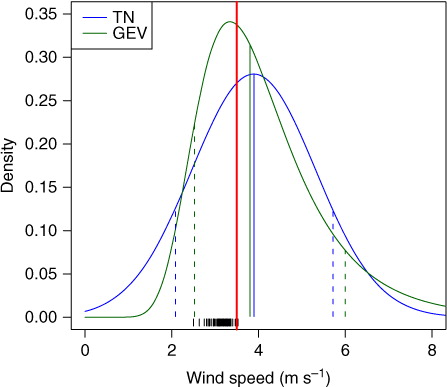
We propose to combine the NR ensemble post-processing framework originally proposed by Gneiting et al. (2005) and later extended by Thorarinsdottir and Gneiting (2010) with results from extreme value theory. That is, we apply a predictive distribution from the GEV family, where the location and scale parameters depend on the ensemble member forecasts. To illustrate the difference between the two NR approaches, Fig. 1 shows the predictive distributions for Frankfurt Airport on 19 March 2011. Both the truncated normal (TN) and the GEV model correct the negative bias and the underdispersion of the ensemble, while the GEV density is less symmetric and exhibits a heavy right tail. We further investigate a regime-switching approach, which issues a TN predictive density when the ensemble median forecast takes a low value and a GEV predictive density for high values of the ensemble median.

Fig. 1 One-day ahead forecasts for daily maximum wind speed at Frankfurt Airport valid on 19 March 2011. The ECMWF ensemble forecasts are indicated in black, the observation in red. The solid blue and green lines indicate the median of the truncated normal (TN) and the GEV predictive distribution, respectively. The dashed lines indicate the corresponding central 80% prediction intervals.

The remainder of the article is organised as follows. In Section 2, the ensemble forecasts and the observational data are introduced. In Section 3, we review the NR technique and describe our extensions using GEV distributions and a regime-switching combination model. Section 4 summarises the probabilistic scores used for estimating the model parameters and evaluating the competing forecasting procedures. In particular, we discuss how appropriately weighted proper scoring rules recently proposed in the economic literature (Diks et al., 2011; Gneiting and Ranjan, 2011) can be used to assess the predictive performance for high wind speeds. In Section 5, we report the results of a case study on daily maximum wind speed over Germany for lead times of 1–3 d with the ensemble issued by the European Centre for Medium-Range Weather Forecasts (ECMWF) from May 2010 to April 2011. We close with a discussion in Section 6.

2. Data

We consider an ensemble forecast with 50 members of near-surface (10-m) wind speed obtained from the global ensemble prediction system of the ECMWF. Ensemble forecasts for lead times up to 10 d ahead are issued twice a day at 00 UTC and 12 UTC, with a horizontal resolution of about 33 km and a temporal resolution of 3–6 hours. To account for uncertainties in the initial conditions and the numerical model, the ensemble members are generated from random perturbations in initial conditions and stochastic physics parametrisation (Molteni et al., 1996; Leutbecher and Palmer, 2008; Pinson and Hagedorn, 2012). The ensemble members are thus statistically indistinguishable and can be treated as exchangeable (Fraley et al., 2010). We restrict our attention to the ECMWF ensemble run initialised at 00 UTC and lead times of 1–3 d. To obtain predictions of daily maximum wind speed, we take the daily maximum of each ensemble member at each grid point location. For instance, one-day ahead forecasts are given by the maximum over lead times of 3, 6, …, 24 hours.

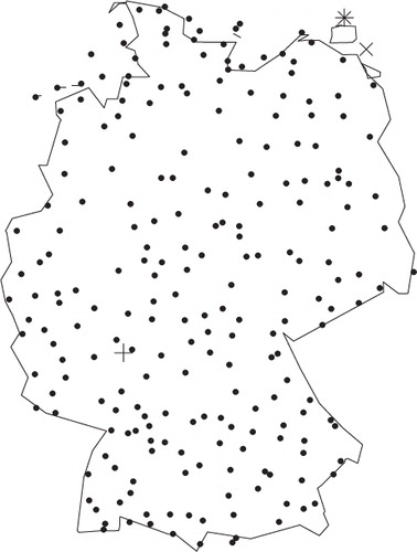
The forecasts are verified over a set of 228 synoptic observation stations over Germany, see Fig. 2. The observations are hourly observations of 10-minute average wind speed which are measured over the 10 minutes before the hour. To obtain daily maximum wind speed, we take the maximum over the 24 hours corresponding to the time frame of the ensemble forecast. In the following, the terms wind speed and daily maximum wind speed are used synonymously. Ensemble forecasts at individual stations are obtained by bilinear interpolation of the gridded model output. The results presented below are based on a verification period from 1 May 2010 to 30 April 2011, consisting of 83220 individual forecast cases. Additionally, we use data from 1 February 2010 to 30 April 2011 to obtain training periods of equal lengths for all days in the verification period and for model selection purposes.

Fig. 2 Map of Germany showing the locations of the 228 synoptic observation stations used in this study. The station at Frankfurt Airport is indicated with +, the station at Greifswalder Oie is indicated with ×, and the station at Kap Arkona is indicated with *.

3. NR prediction models

The NR methodology was originally developed for sea-level pressure and surface temperature under a normal predictive distribution (Gneiting et al., 2005), see also Hagedorn et al. (2008) and Kann et al. (2009) for further applications. Thorarinsdottir and Gneiting (2010) extend the framework to wind speed using a normal distribution truncated in zero, while Thorarinsdottir and Johnson (2012) apply the same setup to predict gust speeds based on NWP forecasts of wind speed and gust factors. A bivariate normal model for wind vectors is discussed in Schuhen et al. (2012). An NR framework for quantitative precipitation has recently been proposed by Scheuerer (2013) using a GEV model for the precipitation accumulations.

3.1. TN model

Let Y denote wind speed and X ₁, …, X _k the corresponding ensemble member forecasts. The predictive distribution for Y is given by a TN distribution with a cut-off at 0,1

where the location parameter is an affine function of the ensemble forecasts and the scale parameter is an affine function of the ensemble variance with . As the ECMWF ensemble members are exchangeable, we assume that , or (Fraley et al., 2010). The cumulative distribution function of the TN distribution is given by

for z>0, and 0 otherwise, where Φ denotes the cumulative distribution function of the standard normal distribution.

3.2. GEV model

As an alternative to the TN model in (1), we consider a model based on extreme value theory. The cumulative distribution function of the GEV distribution with location parameter µ, scale parameter σ and shape parameter ξ is given by2

This distribution is defined on the set {z∈ℝ :1+ξ(z−μ)/σ>0}, where the parameters satisfy ℝ and σ>0. For ξ>0, G is of Fréchet type with a heavy right tail and it holds that . We obtain the Fréchet type in approximately 99.5% of our forecast cases. We estimate the parameters of the model in (2) without any constraints on the parameter values. It is thus possible to obtain non-zero probabilities of negative wind speed. However, as our data consist of daily maximum wind speeds, we find that this rarely happens in practice. The probability of negative wind speed is larger than 1% in about 0.1% of the forecast cases and it never exceeds 5%.

To link the parameters of the predictive GEV distribution to the ensemble, we apply the Bayesian covariate selection algorithm described in Friederichs and Thorarinsdottir (2012) to the data from 1 February 2010 to 30 April 2010. In this analysis, we assume a constant shape parameter ξ, while the location µ and the scale σ may depend on the ensemble mean and variance,

where μ_i ,σ_i ∈ ℝ for i=0,1,2 and κ_i ,ν_i ∈ {0,1} for i=1,2. For 100000 iterations of the Metropolis within Gibbs algorithm with a burn-in period of 20000 iterations, we obtain very high posterior inclusion probabilities for the mean ensemble forecast while k ₂=1 or v ₂=1 holds for less than 0.1% of the posterior sample for each parameter. In our subsequent predictions for the test set from 1 May 2010 to 30 April 2011, we thus set and under the constraint that σ>0, as the results of Friederichs and Thorarinsdottir (2012) indicate that an identity link on σ results in minimally improved performance compared to the logarithmic link for the estimation procedure described in Section 4.

3.3. Regime-switching combination model

The third model we consider is a regime-switching method which combines the TN approach in (1) and the GEV approach in (2). Conditional on the median of the ensemble predictions,

we either issue a TN or a GEV predictive distribution independently at each station. That is, for a model threshold , we define the predictive distribution by3

Here, the parameters of the TN and GEV models depend on the ensemble forecast as described above. However, we train the TN model only on training data for which it holds that . Similarly, the parameters of the GEV distribution are learned from data where . The model threshold θ is selected by comparing predictive performance over a range of possible thresholds based on the out-of-sample data from 1 February to 30 April 2010. Generally, thresholds between 7 and 8 m s⁻¹ prove optimal which approximately corresponds to the 75th and 85th percentiles of the median ensemble predictions over the verification period. These results are discussed in detail below. Under this model, the probability of negative wind speed is less than 1.4×10⁻⁵ for all forecast cases.

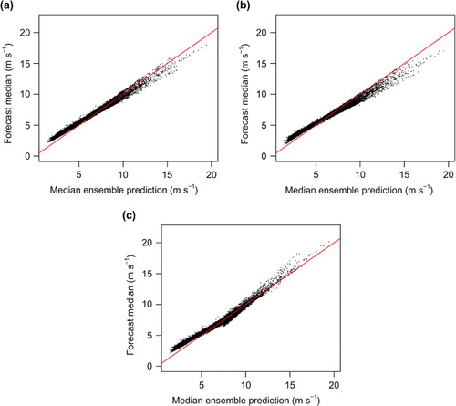
To illustrate the effect of the regime switching in (3), Fig. 3 shows the median of the post-processed predictive distribution as a function of the ensemble median for the three post-processing methods proposed here. While the plots for the TN and the GEV models display a linear though slightly heteroskedastic relationship between the two, this relationship is piecewise linear for the combination method. In particular, as the parameters of the GEV regime are learned from data where only, the median of the post-processed distribution is generally higher than when the GEV distribution is used for all forecast cases.

Fig. 3 The post-processed forecast median for: (a) the truncated normal (TN) model, (b) the generalised extreme value (GEV) model, and (c) the regime-switching combination method as a function of the median ensemble prediction for 20000 randomly selected forecast cases in the test set. The red lines indicate the line x=y.

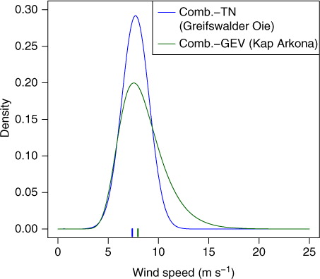
Under the regime-switching framework in (3), stations with similar ECMWF median forecasts might have somewhat different post-processed forecasts when these fall close to the limit θ, see the example in Fig. 4. However, as our data set consists of a collection of individual stations that are separated in space, this does not imply discontinuities in the resulting predictions. If a continuous spatial forecast is needed, a single TN or GEV model as presented above might be more appropriate.

Fig. 4 One-day ahead forecasts for daily maximum wind speed at Greifswalder Oie and Kap Arkona under the combination method valid on 19 March 2011. The ECMWF median forecasts are indicated by the short bars. The ECMWF median forecast at Greifswalder Oie is 7.4 m s⁻¹ resulting in a TN predictive distribution, while the ECMWF median forecast of 7.95 m s⁻¹ at Kap Arkona results in a GEV predictive distribution. The locations of the two stations are indicated in Fig. 2.

4. Parameter estimation and prediction verification

The aim of the prediction is to ‘maximize the sharpness of the predictive distribution subject to calibration’ (Gneiting et al., 2007). Calibration is a joint property of the predictive distribution and the associated observation. It essentially requires that the observation is indistinguishable from a random draw from the predictive distribution. Sharpness refers to the concentration of the predictive distribution and is a property of the forecasts only.

Anderson (1996) and Hamill and Colucci (1997) propose verification rank (VR) histograms as a graphical tool to assess the calibration of ensemble predictions. VR histograms show the distribution of the ranks of the observations when pooled within the ordered ensemble predictions. For a calibrated ensemble, the observations and the ensemble predictions should be exchangeable, resulting in a uniform VR histogram. The continuous analogue of the VR histogram is the probability integral transform (PIT) histogram (Dawid, 1984; Gneiting et al., 2007). The PIT is the value of the predictive cumulative distribution function at the realised observation. Again, for calibrated forecasts, the PIT values should follow a uniform distribution.

To quantify the deviation of VR histograms from uniformity, Delle Monache et al. (2006) propose the reliability index Δ. Here, we define Δ to apply equally to VR and PIT histograms and let it be given by:4

where m denotes the number of classes in the histogram, each of which having expected relative frequency 1/m, and f _i denotes the observed relative frequency in class i.

4.1. Proper scoring rules

Scoring rules assign numerical values to forecast–observation pairs and provide summary measures of predictive performance. Forecasting methods can be compared in this manner by averaging their scores over a test set. If the scoring rule evaluates the full predictive distribution, it can simultaneously address calibration and sharpness. A scoring rule is proper if the expected score is minimised when the true distribution of the observation is issued as the forecast (Bröcker and Smith, 2007; Gneiting and Raftery, 2007). Proper scores thus prevent hedging strategies.

Popular examples of proper scoring rules are the logarithmic or ignorance score (Good, 1952),5

where f denotes the density of F and y denotes the corresponding observation, and the continuous ranked probability score (CRPS) (Hersbach, 2000; Gneiting and Raftery, 2007),6

where the distribution F is assumed to have a finite first moment. Again, y denotes the corresponding observation. We furthermore use the absolute error for the point forecast x given by the median of the predictive distribution as a deterministic measure of accuracy. The median of the predictive distribution is the Bayes predictor under the absolute error loss function (Gneiting, 2011). Here, the scoring rules are negatively oriented in that a smaller score denotes a better performance.

4.2. Evaluation of forecasts for high wind speeds

Despite the variety of theoretically justifiable methods to evaluate probabilistic forecasts, it is not obvious how to assess the predictive performance in the tails of the distribution, for example in the case of extreme wind speed observations. A natural approach is to select extreme events while discarding non-extreme events, and to proceed using standard evaluation procedures. However, it can be shown that restricting proper scoring rules to subsets of events results in improper scoring rules. This approach is thus bound to discredit even the most skilful forecasters (Gneiting and Ranjan, 2011). Instead, weighted scoring rules that emphasise specific regions of interest can be constructed.

Gneiting and Ranjan (2011) propose the threshold-weighted continuous ranked probability score (twCRPS),7

where w(z) is a non-negative weight function on the real line. For , the twCRPS reduces to the original CRPS in (6). If the interest lies in the right tail of the distribution, we may set . Note that the CRPS in (6) represents an integral of the Brier score (Brier, 1950) over all possible thresholds. The twCRPS in (7) with thus allows us to simultaneously assess the exceedance probabilities for all thresholds greater or equal to r. Similarly, Diks et al. (2011) propose proper weighted versions of the logarithmic score in (5).

4.3. Optimum score estimation

The framework of proper scoring rules may also be applied to parameter estimation. Following the general optimum score estimation approach of Gneiting and Raftery (2007), the parameters of a distribution are determined by optimising the average value of a proper scoring rule as a function of the parameters over a training set. Optimum score estimation based on the logarithmic score in (5) thus corresponds to maximum likelihood (ML) estimation. Minimum CRPS estimation, that is, optimum score estimation based on the CRPS in (6) provides a robust alternative to ML estimation if closed-form expressions for the CRPS of the distribution family of interest are available.

Following Thorarinsdottir and Gneiting (2010), we estimate the parameters of the TN model using minimum CRPS estimation. Friederichs and Thorarinsdottir (2012) derive a closed-form expression of the CRPS for the GEV distribution and compare ML and minimum CRPS estimation for their analysis of peak wind speed. For our data set, ML estimation proved to be more parsimonious and numerically stable. There is no analytical solution of the corresponding ML minimisation problem (Coles, 2001). However, numerical approximations can be obtained using standard algorithms for any given data set (Prescott and Walden, 1980). For the regime-switching combination model in (3), minimum CRPS estimation is applied for the parameters of the TN distribution and ML estimation for the parameters of the GEV distribution. For all three methods, the parameters are estimated over a rolling training period consisting of the forecast–observation pairs of the last m days. The parameters are estimated regionally in that training data from all stations are pooled together.

5. Results

Here, we present the results for 1–3 d ahead probabilistic forecasts of daily maximum wind speed over Germany produced by the three different post-processing methods presented in Section 3. The verification period covers 1 yr, from 1 May 2010 to 30 April 2011.

5.1. Selection of training period and regime-switching threshold

The results presented here are based on a rolling training period of length m=30 d for all methods. We have also performed the same analysis for training periods of length m=20, 25, …, 50 d. In general, shorter training periods allow for a rapid adaption to changes in environmental conditions while longer training periods reduce the statistical variability in the parameter estimation (Gneiting et al., 2005). We found that the performance scores reported in Table 1 change by less than 1% for the different values of m, and, in accordance with the results of Thorarinsdottir and Gneiting (2010) and Thorarinsdottir and Johnson (2012), we conclude that the methods are robust against changes in m.

Table 1. Mean continuous ranked probability score (CRPS), mean absolute error (MAE), average coverage and width of 80% prediction intervals of probabilistic one-day ahead forecasts of daily maximum wind speed at 228 synoptic stations in Germany from 1 May 2010 to 30 April 2011. The best score for each performance measure is indicated in bold

Forecast	CRPS (m s^−1)	MAE (m s^−1)	Coverage (%)	Width (m s^−1)
Climatology	1.54	2.13	64.4	6.6
Ensemble	1.26	1.44	26.6	1.0
TN	1.05	1.39	80.4	4.0
GEV	1.04	1.39	82.9	4.6
Combination	1.03	1.38	80.8	4.1

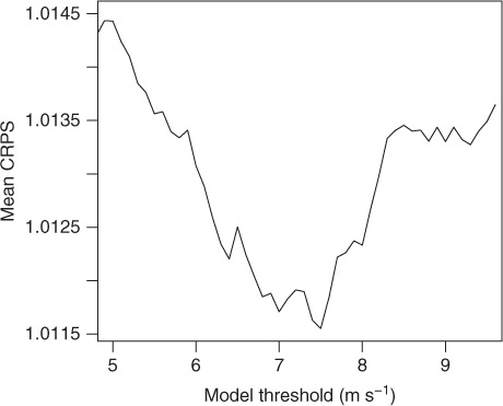
The model threshold θ for the regime-switching combination model in (3) is determined by computing the mean CRPS for a range of threshold values over an out-of-sample training period from 1 February 2010 to 30 April 2010. Using a rolling training period of m=30 d, we obtain the optimal score for θ=7.5 m s⁻¹, see Fig. 5. A sensitivity analysis shows that the results in Table 1 are nearly constant for values of θ between 7 and 8 m s⁻¹ and various choices of m. The threshold of 7.5 m s⁻¹ approximately corresponds to the 80th percentile of the median ensemble predictions in the verification set. Over the verification period, a GEV distribution is used in approximately 18% of the forecast cases.

Fig. 5 Mean continuous ranked probability score (CRPS) for the regime-switching model as a function of the model threshold θ. The results are based on a rolling training period of 30 d during the out-of-sample time period from 1 February 2010 to 30 April 2010.

5.2. One-day ahead predictive performance

We compare the three ensemble post-processing methods discussed above to the raw, unprocessed ECMWF ensemble and a climatological reference forecast. For each day, the climatological reference forecast is obtained from the observed wind speeds in the 30-d training period used for the parameter estimation of the post-processing methods. VR and PIT histograms for the ensemble and the three post-processing methods are shown in Fig. 6. The ECMWF forecasts are underdispersive, with too many observations falling outside the ensemble range. This deficiency has repeatedly been observed for various ensemble prediction systems. Possible causes for the ECMWF ensemble in this case are underdispersiveness of the underlying model, unsatisfactory modelling of the uncertainty using random perturbations, and spatial and temporal interpolation and smoothing issues, see e.g. Hamill and Colucci (1997), Palmer (2002) and Raftery et al. (2005).

Fig. 6 Calibration checks for probabilistic one-day ahead forecasts of wind speed over Germany aggregated over 1 May 2010 to 30 April 2011 and the 228 stations: (a) verification rank (VR) histogram for the ECMWF ensemble forecasts; (b) PIT histogram for the TN model; (c) PIT histogram for the GEV model; (d) PIT histogram for the regime-switching combination technique.

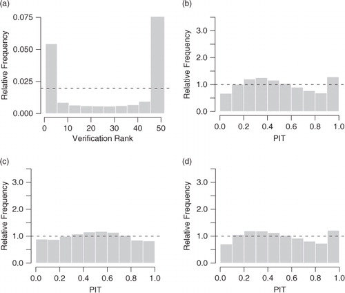
All three post-processing methods significantly improve the calibration of the ensemble. While the GEV forecasts are slightly overdispersive, their PIT histogram shows smaller deviations from uniformity than that of the TN forecasts. The PIT histogram of the combination model resembles the PIT histogram of the TN technique, with minor improvements for large PIT values. The PIT histograms thus indicate that the GEV distributions tend to have minimally too heavy tails, while the upper tails for the TN distributions seem slightly too light. The combination model somewhat compensates for this. Substantial improvements in calibration compared to the raw ensemble are also indicated by values of the reliability index Δ (4). For all observations pooled together, the reliability index of 1.02 for the ECMWF ensemble predictions is reduced to 0.19 for the TN model, 0.12 for the GEV model and 0.16 for the combination model. The post-processing methods further lead to an improvement in local calibration at all observation stations. If the 228 stations are considered individually, the median reliability index of 0.97 for the ensemble predictions reduces to 0.49 for the TN model, 0.53 for the GEV model and 0.48 for the combination model.

Table 1 shows the mean CRPS, the MAE and average coverage and width of 80% prediction intervals for the competing forecasts. Here, the point forecast evaluated by the MAE is given by the median of the corresponding predictive distribution. For calibrated forecasts, the average coverage of 80% prediction intervals should be close to 80% and narrower average prediction intervals indicate sharper forecasts. For discrete distributions such as the ECMWF ensemble and the climatological forecast, the CRPS can be calculated explicitly, see e.g. Berrocal et al. (2008). The CRPS for the TN model and the GEV model is calculated as described in Thorarinsdottir and Gneiting (2010) and Friederichs and Thorarinsdottir (2012), respectively. The ECMWF ensemble predictions outperform the climatological reference forecast and provide sharp prediction intervals at the cost of being uncalibrated. All post-processing methods outperform the ensemble predictions, with the GEV method showing small improvements in mean CRPS compared to the TN method. The regime-switching combination method performs best in terms of both mean CRPS and MAE, slightly improving the results of the GEV method. Note that due to the heavier tails, the GEV model generally results in wider prediction intervals than the TN model.

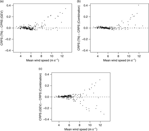
Figure 7 compares the station-specific predictive performance of the individual post-processing models as a function of the site-specific average observed wind speed. Figure 7(a) and (b) indicates that the overall improvements of the GEV and the regime-switching combination model over the TN model are mainly due to improvements at stations with high average observed wind speeds. However, there appears to be no obvious pattern for stations with high average wind speeds when comparing the GEV model and the regime-switching combination model in Fig. 7(c). However, the combination model outperforms the GEV model for most stations with average observed wind speeds below 7 m s⁻¹.

Fig. 7 Station-specific comparisons of the continuous ranked probability score (CRPS) for the three post-processing methods as a function of the average observed daily maximum wind speed at the station. The plots compare (a) the TN and the GEV models, (b) the TN and the regime-switching combination models, and (c) the GEV and the regime-switching combination models. The horizontal dashed lines indicate equal predictive performance.

5.3. One-day ahead performance in the upper tail

With a focus on the performance in the upper tail, Table 2 shows values of the mean twCRPS for the competing forecasts where we have employed the indicator weight function for r=10,12 and 15 m s⁻¹. The threshold values approximately correspond to the 90th, 95th and 98th percentiles of the marginal distribution of the wind speed observations. The twCRPS is here calculated using numerical integration methods. All three post-processing methods improve the ECMWF ensemble predictions, and the GEV approach outperforms the TN method. The regime-switching combination of the two models further improves the performance. Note that the relative improvement over the TN method for the upper tail is comparatively larger than the improvement under the unweighted CRPS in Table 1. Similar rankings hold for any value of r between 10 and 20 m s⁻¹.

Table 2. Mean threshold-weighted continuous ranked probability score (twCRPS) for one-day ahead forecasts of daily maximum wind speed at 228 synoptic stations in Germany from 1 May 2010 to 30 April 2011 using an indicator weight function for different values of r. The best score for each threshold value is indicated in bold

Forecast	r=10	r=12	r=15
Climatology	0.250	0.128	0.045
Ensemble	0.211	0.113	0.043
TN	0.200	0.111	0.042
GEV	0.195	0.107	0.041
Combination	0.191	0.103	0.039

We further consider the threshold-weighted continuous ranked probability skill score (twCRPSS) given by8

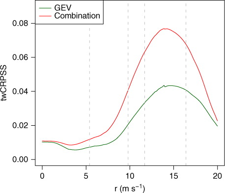
where F _ref denotes the predictive cumulative distribution function of a reference forecast, in our case the TN method. The twCRPSS is positively oriented and can be interpreted as an improvement over the reference forecast. Figure 8 shows the twCRPSS for the GEV and the regime-switching combination method as a function of the threshold r for the indicator weight function, using the TN method as a reference forecast. For all thresholds and both models, the twCRPSS is strictly positive, indicating an improved predictive performance compared to the TN model with the regime-switching combination method showing greater improvement. In general, the score values increase for larger threshold values, with the largest differences obtained for threshold values around 14 m s⁻¹.

Fig. 8 Threshold-weighted continuous ranked probability skill score of probabilistic one-day ahead forecasts of daily maximum wind speed at 228 synoptic stations in Germany from 1 May 2010 to 30 April 2011 as a function of the threshold r in the indicator weight function , using the forecasts produced by the TN method as reference. The grey dashed vertical lines indicate the 50th, 90th, 95th and 99th percentile of the marginal distribution of the observations.

5.4. Performance for longer lead times

For lead times of two and three days, we obtain similar results as above. Table 3 shows the mean CRPS, MAE, and average coverage and width of 80% prediction intervals for those lead times. Compared to the one-day ahead forecasts, forecasts for longer lead times result in slightly less accurate predictions and wider prediction intervals. The ECMWF ensemble predictions exhibit wider prediction intervals compared to the one-day ahead forecasts resulting in small improvements in calibration. However, the ensemble predictions are still underdispersive and the three post-processing methods significantly improve the predictive skill of the ensemble. The differences among the three post-processing models are less pronounced than for one-day ahead forecasts. The results for the mean twCRPS and lead times of two and three days are shown in Table 4. We obtain the same ranking as for the one-day ahead forecasts while the differences in the scores for the three models are small. Note that while the post-processing methods show a slight decline in accuracy from two to three days ahead, the scores for the upper tail of the ensemble are identical for these lead times.

Table 3. Mean continuous ranked probability score (CRPS), mean absolute error (MAE), average coverage and width of 80% prediction intervals of daily maximum wind speed forecasts at 228 synoptic stations in Germany from 1 May 2010 to 30 April 2011. The best score for each performance measure is indicated in bold

Forecast	CRPS (m s^−1)	MAE (m s^−1)	Coverage (%)	Width (m s^−1)
Two-day ahead
Climatology	1.55	2.14	64.4	6.6
Ensemble	1.22	1.47	38.8	1.6
TN	1.07	1.43	80.5	4.1
GEV	1.06	1.43	82.5	4.7
Combination	1.06	1.43	80.6	4.2
Three-day ahead
Climatology	1.55	2.14	64.4	6.6
Ensemble	1.22	1.52	48.0	2.1
TN	1.10	1.47	80.4	4.3
GEV	1.09	1.47	82.3	4.8
Combination	1.09	1.47	80.7	4.3

GEV=generalised extreme value; TN=truncated normal.

The upper half shows results for two-day ahead forecasts, the lower half results for three-day ahead forecasts.

Table 4. Mean threshold-weighted continuous ranked probability score (twCRPS) of daily maximum wind speed forecasts at 228 synoptic stations in Germany from 1 May 2010 to 30 April 2011 using an indicator weight function for different values of r. The best score for each threshold value is indicated in bold

Forecast	r=10	r=12	r=15
Two-day ahead
Climatology	0.250	0.128	0.045
Ensemble	0.209	0.113	0.043
TN	0.202	0.111	0.043
GEV	0.198	0.108	0.041
Combination	0.196	0.106	0.040
Three-day ahead
Climatology	0.250	0.128	0.045
Ensemble	0.209	0.113	0.043
TN	0.204	0.112	0.043
GEV	0.200	0.109	0.041
Combination	0.199	0.107	0.041

GEV=generalised extreme value; TN=truncated normal.

The upper half shows results for two-day ahead forecasts, the lower half shows results for three-day ahead forecasts.

6. Discussion

We propose two extensions to the NR ensemble post-processing approach of Thorarinsdottir and Gneiting (2010) employing GEV predictive distributions for daily maximum wind speed. In a case study over Germany using the exchangeable ECMWF ensemble, all three NR methods significantly improve the calibration as well as the overall skill of the raw ensemble. The best method according to our results is a regime-switching method, where a TN model is applied when we expect low winds, while a GEV framework is used when high winds are expected.

In our GEV approach, we have not accounted for the possibility of the method predicting negative wind speeds. While this rarely happens in our case study, different results are likely to be obtained for less extreme wind variables. In an application to quantitative precipitation, Scheuerer (2013) considers the GEV distribution to be left-censored at zero assigning all mass below zero to exactly zero. This approach seems very appropriate for precipitation, where there is often high probability of zero precipitation. However, it seems less appropriate for wind variables. Instead, one might consider a truncation of the GEV distribution similar to the TN distribution in (1).

The regime-switching combination of the TN and the GEV models offers several starting points for further extensions and potential improvements. For each forecast case, either the TN or the GEV model is selected based on the median ensemble prediction falling below or exceeding a fixed threshold θ. Instead of assuming a fixed threshold value, it might be interesting to develop an adaptive method to automatically estimate θ, for example based on station-specific information or other weather variables. Alternatively, improvements of the predictive performance for extreme events might be achieved by considering a mixture model using a TN distribution for the bulk of the distribution, and an adaptive generalised Pareto distribution (GPD) for the tail. Bentzien and Friederichs (2012) propose such a mixture model for precipitation using lognormal and gamma mixtures for the bulk of the distribution and an adaptive GPD tail which is able to significantly improve the predictive performance for extreme quantiles, see also Frigessi et al. (2002). Similarly, all three methods could be extended by allowing for local adaption of the parameter estimation. This might be obtained with a geostatistical approach analogous to Kleiber et al. (2011a, b), where the spatially varying parameters are estimated locally and interpolated to locations without available observations.

When assessing the predictive performance in the upper tail, we have focused on the twCRPS with a simple indicator weight function. Under this weight function, it is not possible to distinguish between forecasts with the same behaviour on , but different behaviour on . Following Gneiting and Ranjan (2011), we have also performed our analysis using weight functions of the form , where denotes the cumulative distribution function of a normal distribution with mean µ _r and variance . For example, we might set and , or , where S ² is the sample variance of the wind speed observations during the out-of-sample training period from 1 February to 30 April 2010. The average values of the twCRPS using these weight functions result in the same ranking and in comparable relative improvements as reported above for the indicator weight function. We have therefore focused on the indicator weight function which is computationally less demanding.

Our data set does not contain any missing forecasts or observations. Single missing observations would presumably only have negligible effects on the predictions since observations from all stations are pooled together for the parameter estimation. Bayesian adaptions of ensemble post-processing methods as proposed by Bishop and Shanley (2008) and Di Narzo and Cocchi (2010) allow for incorporation of uncertainty in both observations and parameters and might help to overcome the effects of missing data. However, they are computationally quite demanding compared to the frequentist approach taken in this work and might thus be infeasible for a large number of stations and observations. For further relevant work, see also Crochet (2004) and references therein.

7. Acknowledgements

The authors thank Tilmann Gneiting and Michael Scheuerer for helpful discussions and for providing the observation data. The comments of two reviewers greatly improved the quality of this article. The support of the Volkswagen Foundation through the project ‘Mesoscale Weather Extremes – Theory, Spatial Modelling and Prediction (WEX-MOP)’ and Statistics for Innovation sfi ² in Oslo is gratefully acknowledged.

References

- Anderson J. L . A method for producing and evaluating probabilistic forecasts from ensemble model integrations. J. Clim. 1996; 9: 1518–1530.
- Bao L , Gneiting T , Grimit E. P , Guttorp P , Raftery A. E . Bias correction and Bayesian model averaging for ensemble forecasts of surface wind direction. Mon. Weather Rev. 2010; 138: 1811–1821.
- Bentzien S , Friederichs P . Generating and calibrating probabilistic quantitative precipitation forecasts from the high-resolution NWP model COSMO-DE. Weather Forecast. 2012; 27: 988–1002.
- Berrocal V. J , Gneiting T , Raftery A. E . Probabilistic quantitative precipitation field forecasting using a two-stage spatial model. Ann. Appl. Stat. 2008; 2: 1170–1193.
- Bishop C. H , Shanley K. T . Bayesian model averaging's problematic treatment of extreme weather and a paradigm shift that fixes it. Mon. Weather Rev. 2008; 136: 4641–4652.
- Brier G. W . Verification of forecasts expressed in terms of probability. Mon. Weather Rev. 1950; 78: 1–3.
- Bröcker J , Smith L. A . Scoring probabilistic forecasts: the importance of being proper. Weather Forecast. 2007; 22: 382–388.
- Celik A. N . A statistical analysis of wind power density based on the Weibull and Rayleigh models at the southern region of Turkey. Renew. Energ. 2004; 29: 593–604.
- Coles S . An Introduction to Statistical Modeling of Extreme Values. 2001; Springer, London.
- Courtney J. F , Lynch P , Sweeney C . High resolution forecasting for wind energy applications using Bayesian model averaging. Tellus A. 2013; 65: 19669.
- Crochet P . Adaptive Kalman filtering of 2-metre temperature and 10-metre wind-speed forecasts in Iceland. Meteorol. Appl. 2004; 11: 173–187.
- Dawid A. P . Statistical theory: the prequential approach. J. Roy. Stat. Soc. A. 1984; 147: 278–292.
- Delle Monache L , Hacker J. P , Zhou Y , Deng X , Stull R. B . Probabilistic aspects of meteorological and ozone regional ensemble forecasts. J. Geophys. Res. 2006; 111: D24307.
- Diks C , Panchenko V , van Dijk D . Likelihood-based scoring rules for comparing density forecasts in tails. J. Econ. 2011; 163: 215–230.
- Di Narzo A. F , Cocchi D . A Bayesian hierarchical approach to ensemble weather forecasting. J. Roy. Stat. Soc. C. 2010; 59: 405–422.
- European Wind Energy Association. Wind in power: 2012 European statistics. 2012. Online at: http://www.ewea.org/fileadmin/files/library/publications/statistics/Wind_in_power_annual_statistics_2012.pdf.
- Fraley C , Raftery A. E , Gneiting T . Calibrating multimodel forecast ensembles with exchangeable and missing members using Bayesian model averaging. Mon. Weather Rev. 2010; 138: 190–202.
- Friederichs P , Thorarinsdottir T. L . Forecast verification for extreme value distributions with an application to probabilistic peak wind prediction. Environmetrics. 2012; 7: 579–594.
- Frigessi A , Haug O , Rue H . A dynamic mixture model for unsupervised tail estimation without threshold selection. Extremes. 2002; 5: 219–235.
- Garcia A , Torres J. L , Prieto E , De Francisco A . Fitting wind speed distributions: a case study. Sol. Energ. 1998; 62: 139–144.
- Genton M , Hering A . Blowing in the wind. Significance. 2007; 4: 11–14.
- Gneiting T . Making and evaluating point forecasts. J. Am. Stat. Assoc. 2011; 106: 746–762.
- Gneiting T , Balabdaoui F , Raftery A. E . Probabilistic forecasts, calibration and sharpness. J. Roy. Stat. Soc. B. 2007; 69: 243–268.
- Gneiting T , Raftery A. E . Weather forecasting with ensemble methods. Science. 2005; 310: 248–249.
- Gneiting T , Raftery A. E . Strictly proper scoring rules, prediction, and estimation. J. Am. Stat. Assoc. 2007; 102: 359–378.
- Gneiting T , Raftery A. E , Westveld A. H , Goldman T . Calibrated probabilistic forecasting using ensemble model output statistics and minimum CRPS estimation. Mon. Weather Rev. 2005; 133: 1098–1118.
- Gneiting T , Ranjan R . Comparing density forecasts using threshold- and quantile-weighted scoring rules. J. Bus. Econ. Stat. 2011; 29: 411–422.
- Good I. J . Rational decisions. J. Roy. Stat. Soc. B. 1952; 14: 107–114.
- Hagedorn R , Hamill T. M , Whitaker J. S . Probabilistic forecast calibration using ECMWF and GFS ensemble reforecasts. Part I: two-meter temperatures. Mon. Weather Rev. 2008; 136: 2608–2619.
- Hamill T. M , Colucci S. J . Verification of Eta-RSM short-range ensemble forecasts. Mon. Weather Rev. 1997; 125: 1312–1327.
- Hersbach H . Decomposition of the continuous ranked probability score for ensemble prediction systems. Weather Forecast. 2000; 15: 559–570.
- Kann A , Wittmann C , Wang Y , Ma X . Calibrating 2-m temperature of limited-area ensemble forecasts using high-resolution analysis. Mon. Weather Rev. 2009; 137: 3373–3387.
- Kleiber W , Raftery A. E , Gneiting T . Geostatistical model averaging for locally calibrated probabilistic quantitative precipitation forecasting. J. Am. Stat. Assoc. 2011a; 106: 1291–1303.
- Kleiber W , Raftery A. E , Baars J , Gneiting T , Mass C. F , co-authors . Locally calibrated probabilistic temperature forecasting using geostatistical model averaging and local Bayesian model averaging. Mon. Weather Rev. 2011b; 139: 2630–2649.
- Lei M , Shiyan L , Chuanwen J , Hongling L , Yan Z . A review on the forecasting of wind speed and generated power. Renew. Sust. Energ. Rev. 2009; 13: 915–920.
- Leutbecher M , Palmer T. N . Ensemble forecasting. J. Comput. Phys. 2008; 227: 3515–3539.
- Molteni F , Buizza R , Palmer T. N . The ECMWF ensemble prediction system: methodology and validation. Q. J. Roy. Meteorol. Soc. 1996; 122: 73–119.
- Palmer T. N . The economic value of ensemble forecasts as a tool for risk assessment: from days to decades. Q. J. Roy. Meteorol. Soc. 2002; 128: 747–774.
- Palutikof J. P , Brabson B. B , Lister D. H , Adcock S. T . A review of methods to calculate extreme wind speeds. Meteorol. Appl. 1999; 6: 119–132.
- Pinson P . Adaptive calibration of (u, v)-wind ensemble forecasts. Q. J. Roy. Meteorol. Soc. 2012; 138: 1273–1284.
- Pinson P , Chevallier C , Kariniotakis G. N . Trading wind generation from short-term probabilistic forecasts of wind power. IEEE Trans. Power Syst. 2007; 22: 1148–1156.
- Pinson P , Hagedorn R . Verification of the ECMWF ensemble forecasts of wind speed against analyses and observations. Meteorol. Appl. 2012; 19: 484–500.
- Prescott P , Walden A. T . Maximum likelihood estimation of the parameters of the generalized extreme-value distribution. Biometrika. 1980; 67: 723–724.
- Raftery A. E , Gneiting T , Balabdaoui F , Polakowski M . Using Bayesian model averaging to calibrate forecast ensembles. Mon. Weather Rev. 2005; 133: 1155–1174.
- Scheuerer M. Probabilistic quantitative precipitation forecasting using ensemble model output statistics. Q. J. Roy. Meteorol. Soc. 2013. Online at: http://onlinelibrary.wiley.com/doi/10.1002/qj.2183/abstract.
- Schuhen N , Thorarinsdottir T. L , Gneiting T . Ensemble model output statistics for wind vectors. Mon. Weather Rev. 2012; 140: 3204–3219.
- Sloughter J. M , Gneiting T , Raftery A. E . Probabilistic wind speed forecasting using ensembles and Bayesian model averaging. J. Am. Stat. Assoc. 2010; 105: 25–35.
- Sloughter J. M , Gneiting T , Raftery A. E . Probabilistic wind vector forecasting using ensembles and Bayesian model averaging. Mon. Weather Rev. 2013; 141: 2107–2119.
- Thorarinsdottir T. L , Gneiting T . Probabilistic forecasts of wind speed: ensemble model output statistics by using heteroscedastic censored regression. J. Roy. Stat. Soc. A. 2010; 173: 371–388.
- Thorarinsdottir T. L , Johnson M. S . Probabilistic wind gust forecasting using non-homogeneous Gaussian regression. Mon. Weather Rev. 2012; 140: 889–897.