The performance of FLake in the Met Office Unified Model

Abstract

We present results from the coupling of FLake to the Met Office Unified Model (MetUM). The coupling and initialisation are first described, and the results of testing the coupled model in local and global model configurations are presented. These show that FLake has a small statistical impact on screen temperature, but has the potential to modify the weather in the vicinity of areas of significant inland water. Examination of FLake lake ice has revealed that the behaviour of lakes in the coupled model is unrealistic in some areas of significant sub-grid orography. Tests of various modifications to ameliorate this behaviour are presented. The results indicate which of the possible model changes best improve the annual cycle of lake ice. As FLake has been developed and tuned entirely outside the Unified Model system, these results can be interpreted as a useful objective measure of the performance of the Unified Model in terms of its near-surface characteristics.

• coupled model
• surface exchange
• inland water
• lake ice
• FLake
• MetUM

1. Introduction

The Met Office Unified Model (MetUM, Davies et al., 2005), including the Joint UK Land Environment Simulator (JULES) surface-exchange scheme (Best et al., 2011; Clark et al., 2011), divides the earth's surface into land and sea. The surface exchange on land points is further subdivided, in almost all model configurations, into separate calculations on each type of land surface (‘tile’) represented in JULES. Each tile has its own defined properties of roughness length, canopy fraction, canopy height, and so on. Results of these calculations are weighted by tile fraction and summed to give gridbox properties. JULES makes provision for diffusive heat flux into the land surface, with the possible buffering of the atmosphere-surface exchange by an intermediate ‘canopy’ layer coupled radiatively to the land surface. Heat exchange between the atmospheric surface layer and this canopy is not limited by the diffusive rate based on its thermal properties; instead the entire canopy mass is assumed to be available for thermal interaction. The atmosphere and the surface/canopy are coupled implicitly (Best et al., 2004).

One tile type within JULES is that of inland water, often referred to as the lake tile. While JULES models surface exchange on all tiles similarly, in reality inland water behaves very differently from other, solid land-cover types, and in many ways is more similar to the sea. Thermal exchange between the atmosphere and lakes may be controlled by turbulent processes both above and below the interface, and the upper portions of a lake can behave similarly to an inverted atmospheric boundary layer. This analogy has been developed at length by Zilitinkevich (1991), in a work which also describes the INOZ one-dimensional model for the numerical solution of the seasonal temperature characteristics of inland water bodies. The efficiency of lake–atmosphere turbulent exchange means that non-frozen lake surfaces are observed to exhibit a much smaller diurnal temperature variation than solid land surfaces.

It should be noted that the inland-water tile fraction is also used to indicate the presence of rivers. These features are more turbulent, and less suitable for one-dimensional modelling, even than lakes. In future, it may be possible to have separate tiles for lakes and rivers, enabling them to be modelled differently.

The correct representation of lake-surface behaviour is important for accurate Numerical Weather Prediction (NWP). The lake model FLake has been developed by a similar approach to that of INOZ, as a parametrisation of lake properties for NWP (Mironov, 2008; Mironov et al., 2010). Principally, this means providing an accurate surface temperature, although to do this much of the physical behaviour of lakes such as wind stirring, convection, freezing, and so on must be considered. Here, we describe the method and results of coupling FLake to MetUM.

Lake–atmosphere interaction is of wider interest besides NWP. Lake modelling for water quality or other purposes has recognised the influence of atmospheric forcing. Attempts have been made to incorporate this into lake studies by simpler, broader scale input compared to that of coupling with a full atmospheric model (e.g. George and Taylor, 1995). The additional detail and insight into lake response, which may be derived from an operational coupled model, is of interest to water companies and others. The biological aspect of lake turbidity may interact with or feed back on temperature structure (Paerl and Huisman, 2008). The possibility of future modelling (or assimilation, Potes et al., 2011) of biological or other lake turbidity is an interesting prospect.

More generally, as a model designed for NWP, FLake does not yet interact with the carbon cycle or indeed the hydrological cycle (the lake depth is fixed by default, and the energy budget does not consider changes in lake temperature caused by river influx or efflux). The importance of lakes in climate has recently been described, for example, by Williamson et al. (2009, and others in that special issue). More sophisticated lake modelling for climate purposes, accounting for the thermal, hydrological and carbon aspects together, ought to be considered in future. It is possible that such developments may be built into a future version of FLake. A prerequisite is the integration of lakes into the network of rivers and other lateral water movement on land.

2. Using FLake in MetUM

2.1. Coupling

The FLake code is quite small, and for standalone use is divided into two main parts, FLake and SfcFlx, which calculate the lake properties and the lake-surface fluxes, respectively. The SfcFlx section is unused when FLake is coupled to MetUM.

The coupling of FLake to MetUM follows the coupling to JULES described by Rooney and Jones (2010) in that, to preserve the implicit surface-temperature calculation in JULES, the surface-temperature output from FLake is not used directly in MetUM. Instead, the lake temperature distribution is drawn upon to provide a subsurface temperature and effective thermal conductivity, which are used in place of the equivalent ‘solid’ subsurface properties in the implicit calculation. The surface flux passed to the soil is also restricted to the fraction-weighted sum of fluxes to each tile except inland water.

FLake requires two components of heat flux as input, the first is the net turbulent and long-wave heat flux at the lake surface, and the second is the downwelling short-wave irradiance, which is supplied together with an albedo. The fluxes are partitioned in this manner because the short-wave irradiance is allowed to penetrate to some depth into the lake, through a parametrisation which makes use of an extinction coefficient. FLake behaviour is sensitive to the value of this coefficient (Potes et al., 2012), which is unfortunately not yet specified in any detail on the global scale. The FLake reference value of the extinction coefficient for water, γ=3 m⁻¹, is set as the default.

To achieve an energy balance in FLake, it is important that the albedo value is the same as that used in MetUM. This is done by computing the albedo directly from the downwelling and net lake-tile short-wave fields in the radiation code in MetUM, and passing the result to FLake. The default unfrozen albedo for the lake tile in MetUM is 0.06. For frozen lakes, the snow-free albedo is calculated as a function of the tile surface temperature which is the same as that of Mironov et al. (2010, equation 33).

The FLake snow scheme is not used. Snowdepth on the lake tile is calculated by the JULES snow scheme and passed to FLake with other prognostics for use in thermodynamic calculations. The snowdepth output by FLake is discarded as a precaution. Another important point is that FLake calculates snow and ice melt, and so the adjustment of the surface energy balance within JULES to take account of surface melting processes must be removed before the net surface heat flux is passed to FLake. Without this step, FLake lacks the energy to melt lake ice in spring.

In the absence of snow cover, JULES assigns a fixed value for the roughness length z ₀ to the inland-water tile (as with other non-vegetated tiles) for surface-exchange calculations. In the MetUM configurations described below, the lake-tile value is z ₀=1×10⁻⁴ m. JULES reduces the roughness length in the presence of snow cover (which would accumulate on a frozen lake) but not below a limit of 5×10⁻⁴ m. Thus, the inland-water roughness length is effectively fixed in the default configurations used here.

2.2. Lake depth

Kourzeneva and Braslavsky (2005) state that the lake depth is the parameter to which FLake is most sensitive. A lake-depth dataset, and accompanying FORTRAN routines to generate a representative gridbox lake depth, have been provided as part of the FLake download package. The representative lake depth for a gridbox may need to parametrise approximately the bathymetry of several lakes or other water bodies (including rivers), which make up the inland-water fraction of that gridbox. The statistical procedure used to produce such a representative depth is described in detail by Kourzeneva (2010). Although thousands of lake depths are collated into the FLake dataset, many times that number remain unknown. Suggested methods of producing a more complete dataset include statistical methods based on geology and physical geography (Sobek et al., 2011), or even data-assimilation techniques (Balsamo et al., 2010).

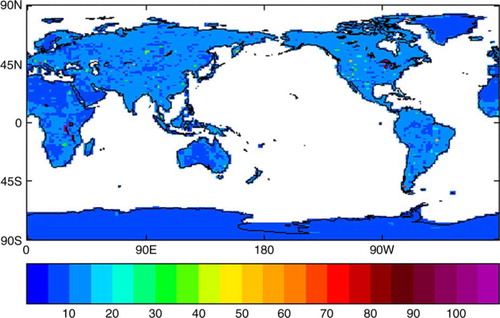
The FLake database routine ProjectLake takes the lat.-long. coordinates of the vertices of a polygon as input, and returns the optimum lake depth inside the polygon. For a rectangular MetUM grid, the program is given the four corners of each gridbox in turn, and the output is combined to produce a file containing the required global data in a single array. For present use, the lake depths generated have been bounded between the limits of 5 and 100 m. A plot of the resulting depth field is shown in Fig. 1.

Fig. 1 Lake-depth (m) for climate testing, generated using FLake software and then bounded between 5 m and 100 m.

2.3. Initialisation

Kourzeneva et al. (2012) have developed a global dataset of lake properties for initialisation of NWP models, by running FLake globally with various lake depths, forced by reanalysis and other data. They also state that high correlations are expected between long-term mean lake temperatures and soil temperatures. A lake-climatology dataset has not yet been implemented in MetUM for lake initialisation, and FLake variables are presently initialised based on the properties of the surface and soil at the same gridpoint.

At present, the soil column in MetUM is divided vertically into four layers with thicknesses of 0.1, 0.25, 0.65 and 2.0 m from the surface downward, making a total column depth of 3.0 m. The lake mixed-layer temperature is initialised from the temperature of the first soil level and constrained to be at least 0.1 K above 0°C. The lake mean temperature is set to the mean temperature of the soil column, but constrained to be between the mixed-layer temperature and 0°C with a margin of at least 0.05 K.

If the column-mean soil temperature, top-level soil temperature and surface temperature are all above 0°C then the ice thickness at that gridpoint is initialised to zero. If either of those soil temperatures is below 0°C, then lake-ice thickness h _i is initialised according to1 where T _m is 0°C, and h _s and T _s are the thickness and mean temperature, respectively, of either the whole soil column or the top soil level (with the first of these taking precedence). Equation (1) is empirical and gives reasonable lake-ice thicknesses in MetUM. Ground frost-penetration depth and lake-ice thickness have previously been linked through proxies such as the freezing index (Frauenfeld et al., 2007).

If only the surface temperature is below 0°C, then the ice thickness is initialised to twice the value of the minimum ice thickness parameter in FLake, h_Ice_min_flk=1.0×10⁻⁹ m. The ice thickness is also constrained to not exceed the maximum ice thickness parameter in FLake, H_Ice_max=3.0 m. From (1), the ice thickness will reach this limit at a column-mean soil temperature of 248.2 K.

3. Results with standard model configurations

3.1. UKV model

MetUM-FLake has been trialled at high resolution, in an extended spin-up run of the UK 1.5 km variable-resolution model (UKV, Tang et al., 2012). This is a 70-level model on a grid which varies from 4 km in the outer region to 1.5 km in the inner region. The domain is shown in Fig. 2, although as the model is based on a grid with a rotated pole, the domain is not rectangular in true coordinates. Similarly, the inner domain is shown in Figs. 3 and 4. The outer region extends from approximately 17°W to 8°E and 46°N to 61°N. The inner region extends from approximately 13°W to 4° and 48° to 59°N.

Fig. 2 Inland-water tile fraction in the UKV. Zero fraction is shown as black, other values up to 1 are shown on the colour scale. The model domain is as described in Section 3.1. Note that the stretched model grid produces distortion around the edges of the plot, e.g., the thinning of the Finistère peninsula.

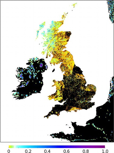
Fig. 3 Gridbox-mean surface temperature, T* (K), around the 8/9 April 2011. (a) T* at 12 UTC on 8 April, MetUM-FLake; (b) T* at 00 UTC on 9 April, MetUM-FLake; (c) T* difference at 00 UTC on 9 April, MetUM-FLake minus control.

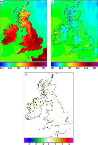
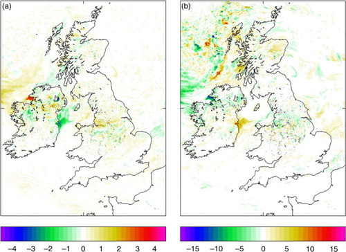
Fig. 4 MetUM-FLake minus control: (a) screen temperature (K) and (b) relative humidity (%) at 6 UTC on 24 March 2011.

Parallel MetUM-FLake and control runs were performed, with the same lateral boundary conditions taken from a run of the Global Model. The trial described here was the final one of a small number, which were useful in testing the MetUM-FLake set-up and highlighting remaining problems.

The inland-water tile fraction in the UKV is shown in Fig. 2. This figure demonstrates the slightly unusual nature of the UKV tile-fraction ancillary, in that the mainland-Britain part is based on the 25 m-resolution dataset from the Centre for Ecology and Hydrology (CEH, Fuller et al., 1994) which is different, and of higher resolution, to the International Geosphere–Biosphere Programme dataset (IGBP, Loveland et al., 2000) used for the rest of the domain. The result for inland water is that large areas of Britain have a small but non-zero fraction, whereas continental Europe and, particularly, Ireland tend to have a more polarised distribution, with small areas of high fraction embedded in a background of predominantly zero fraction.

The trial starting point was 1 January 2011, and MetUM-FLake and a control were run for several months. The lake tile in the control had ‘Neon’ lake settings, which attempt to emulate the heat-exchange characteristics of a water body using an on-tile canopy of high heat capacity. These settings are so called since they were originally used in the Neon tactical decision aid (Fox et al., 2010), although they were previously referred to as ‘JULES-ml’ by Rooney and Jones (2010). The MetUM-FLake run did not use a lake-depth ancillary as such a dataset had not been generated before the start of these extended runs. Instead, the default setting of 5 m lake depth was used for the entire domain.

Two examples from these runs have been chosen to illustrate the potential effect of including FLake. These instances, in March and April 2011, occur during anticyclonic periods over the United Kingdom, and the settled conditions at these times appear to be favourable for amplifying the observed near-surface effects.

Figure 3 shows an example of the effect of FLake in moderating the surface temperature, T*, as observed in this trial. Figure 3a and b shows the gridbox mean T* in two dumps 6 hours apart, at midday on 8 April 2011 and midnight on 9 April 2011. It is evident that, for example, the lake-surface temperature for Lough Neagh in Northern Ireland does not change by nearly as much as the surrounding land surface over this period. Strikingly, at this time in the morning, this water body and others in the west of Ireland have a higher surface temperature in the model than heavily urbanised areas in England. Figure 3c shows the difference between MetUM-FLake and the control at the later time, indicating that the maintained warming in Ireland may have a contribution of as much as 3 K which is attributable to FLake. The weaker, opposite signal in some parts of Scotland indicates that this difference depends to some extent on the weather history at each location, rather than being entirely a simple moderation of the land-surface response.

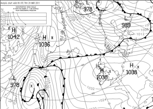
Another potentially interesting lake effect is evident in Fig. 4. This shows differences in screen-level temperature and relative humidity at 6Z on 24 March 2011. In general these differences are of opposite sign, merely indicating small differences in temperature between the two runs. However, there is a small area of much colder and drier air, around the eastern shore of Lough Neagh. The analysis chart for this time, see Fig. 5, shows an anticyclone over the British Isles, and in fact for large areas from Northern Ireland to SW Scotland the relative humidity was at or near 100% in both runs. The small area of cooling is associated with a drop below saturation in the MetUM-FLake run, possibly caused by advection of slightly warmer air off the lake, which has then allowed the temperature on the shore to drop by a few degrees through radiative cooling. This may be an example of the modification of weather in the locality of lakes, caused by the contrast in properties between inland water and other surface types.

Fig. 5 Section of analysis chart at 6 UTC on 24 March 2011.

3.2. Global climate model

MetUM-FLake has also been tested in a 10-yr climate run (beginning in September 1981). FLake and control model runs were based on the MetUM Global Atmosphere 4.0 configuration (Walters et al., 2013). This uses a global-domain climate model, see Fig. 6, at N96 (192 gridpoints E–W, 145 gridpoints N–S) with 85 levels in the vertical, 50 of which are below 18 km, up to a model lid at 85 km. The FLake run used the initialisation and global lake-depth ancillary described in Section 2.

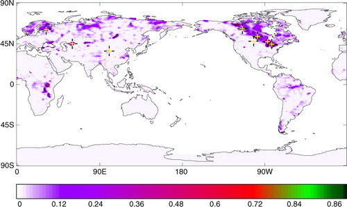
Fig. 6 Lake fraction in MetUM, global climate model domain. The positions of the eight locations examined in detail are marked with yellow-on-black crosses and listed in Table 1.

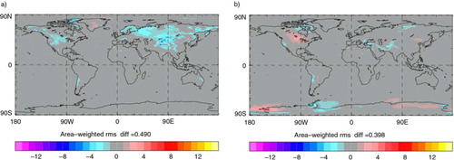
Figures 7 and 8 show screen-temperature comparisons in summer and winter, respectively, between the control run, MetUM-FLake, and climatology from CRUTEM3 (Brohan et al., 2006). In summer, the most significant feature is a cooling along the edge of the Canadian Shield, and stretching west from the Laurentian Great Lakes. The fraction of the lake tile in MetUM is significantly greater than zero over large areas of the Canadian Shield, as shown in Fig. 6. This cooling has the beneficial effect of slightly reducing the peak value of the summertime warm bias in the United States. The warming in the Antarctic is not directly connected with the model change since Antarctica and much of Greenland are designated as surface-type ‘land ice’, which always has a tile fraction of unity in present configurations of MetUM. We speculate that this warming is due to a change in circulation patterns between the two model runs, an effect that may possibly be reduced if the run times were extended.

Fig. 7 Ten-year mean 1.5 m temperature (K), summer months June, July and August: (a) MetUM-FLake mean temperature; (b) MetUM-FLake minus MetUM control; (c) MetUM control minus climatology from CRUTEM3 (Brohan et al., 2006); and (d) MetUM-FLake minus climatology from CRUTEM3.

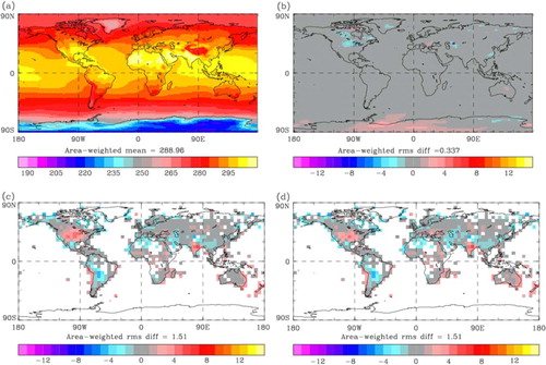
Fig. 8 Ten-year mean 1.5 m temperature (K), winter months December, January and February: (a) MetUM-FLake mean temperature; (b) MetUM-FLake minus MetUM control; (c) MetUM control minus climatology from CRUTEM3 (Brohan et al., 2006); and (d) MetUM-FLake minus climatology from CRUTEM3.

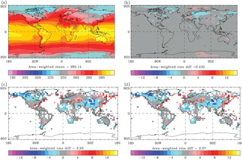
In winter, the screen-temperature changes caused by FLake are both more pronounced and more varied, with cooling over north-western Eurasia, a slight warming around Germany, and a warming–cooling dipole across China, for instance. The overall effect of these changes on model performance does not seem to be very significant, other than an increased cold bias in the Nordic countries and northern Canada.

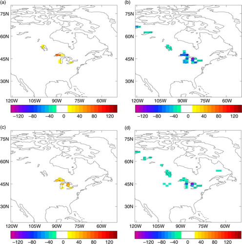
Particularly in the region of the Great Lakes, MetUM-FLake causes large differences in the surface energy balance, as shown in Fig. 9. This figure shows the differences in atmospheric heat fluxes and net downwelling long-wave irradiance at the surface, as well as the difference in screen temperature. (These changes are also evident to a lesser degree in one other gridpoint in the vicinity of the Aral Sea.) The net downwelling short-wave irradiance at the surface is not shown, and does not display any large perturbation unlike the other fluxes. The change in the long-wave balance reflects the fact that the lake surfaces are colder with FLake in this configuration, and this appears to mainly inhibit evaporation. The resultant of the radiative and turbulent fluxes indicates that there is a much greater ‘ground’ heat flux in MetUM-FLake than in the control. This is probably because the parametrised turbulent heat flux in FLake results in a much more efficient transport of energy into the lake body, lowering the surface temperature and perturbing the surface energy balance. Despite the availability of moisture for evaporation, the lowered temperature seems to reduce the mean upward latent heat flux more readily than sensible heat flux. In this case, the change in latent heat flux is greater in magnitude, as well as of opposite sign to the change in sensible heat flux. Subin et al. (2012, see also references therein) note that a reduction in latent heat flux has been observed previously upon the addition of lake-modelling components to atmospheric or general circulation models. Lofgren (1997) attributes such an effect over the Great Lakes to greater atmospheric moisture convergence, as the cooler surface temperature enhances condensation processes over the lakes in spring and summer. As in that study, the changes in the surface energy balance here are not strictly confined to the same grid boxes directly over the lakes, perhaps indicating that local circulatory effects are also induced from the change in the lake-surface energy balance. Related points will be discussed further in the next section.

Fig. 9 Differences in the surface energy balance, MetUM-FLake minus MetUM control, zoomed in to the area around the Laurentian Great Lakes. Fields shown are means for the summer (June, July and August) period. (a) Sensible heat flux (W m⁻²), upward positive; (b) latent heat flux (W m⁻²), upward positive; (c) net downwelling surface long-wave irradiance (W m⁻²); and (d) 1.5 m temperature (K).

To look in more detail at FLake behaviour in the global model, MetUM-FLake and control global climate experiments were run for 40 months from September 1981 to January 1985, retaining monthly timeseries of FLake fields. These used the same model configuration and initialisation as the 10-yr climate runs. Examination of the lake-ice thickness field in these timeseries revealed that there were some locations, for example, in the United States and in China, where lake ice persisted throughout one or more summers, at odds with the expectations from climatology, see below. As FLake has been developed outside the MetUM system, it is hypothesised that this behaviour is a result of features of the forcing data passed to FLake from MetUM. One possible source of variation is the forcing wind stress, as this is a known sensitivity (Subin et al., 2012), and may be more subject to variation between models than more critical or verifiable fields such as surface temperature. In the next section, we describe a range of model tests that were carried out to explore FLake behaviour and sensitivity within MetUM, to try and address this issue.

4. Results of modifications to the MetUM-FLake system

4.1. Modelling concerns and modifications

Some specific points of concern for FLake and lake–atmosphere coupling were discussed at the 2012 Workshop on the Parametrization of Lakes in Numerical Weather Prediction and Climate Modelling (http://netfam.fmi.fi/Lake12/index.html). These include:The relaxation constant C _rc is the coefficient in the scaling relationship which gives the relaxation timescale for thermocline adjustment in terms of thermocline stability, the dominant velocity scale and stratified-layer depth (Mironov et al., 2010, equation 27).

Sensitivity of lake properties to roughness length z ₀ has also been discussed by Subin et al. (2012), who found a trend of reducing surface temperature with increasing local z ₀ for non-frozen lakes, which was associated with increasing evaporation. They conclude that careful treatment of lake aerodynamic roughness lengths is required if large biases in surface fluxes and surface temperatures are to be avoided.

Arising from these considerations, a set of modifications to MetUM-FLake was composed and tested over the 40-month period of the original experiments. The modifications proposed were:Regarding change (B), it was noticed that two specific locations displaying persistent ice problems were also in regions of relatively high orographic roughness, see below. These were the locations numbered 5 and 8 in Table 1. They are referred to as Lake Sakakawea and Qinghai Lake, respectively. (Lake Sakakawea is in fact a reservoir created by a dam.)

Table 1. Characteristics of points extracted for month-by-month evaluation

No.	Name	Lat.	Long.	Lake fraction	Lake depth (m)	Orographic height (m)	Orographic z 0 (mm)
1	Great Slave Lake	61.59	−114.58	0.68	5.0	212.2	2.6
2	Lake Winnipeg	53.01	−98.03	0.62	5.0	238.6	1.8
3	Lake Superior	47.35	−86.99	0.95	100.0	267.1	11.3
4	Lake Huron	44.58	−82.54	0.98	70.0	225.6	5.9
5	Lake Sakakawea	47.80	−102.31	0.03	27.0	706.9	10.4
6	Aral Sea	45.00	60.00	0.98	10.0	57.3	2.0
7	Lake Ladoga	60.86	31.53	0.60	7.0	65.8	6.0
8	Qinghai Lake	36.91	100.23	0.08	18.0	3691.0	65.0

The locations are also plotted in Fig. 6. The model data are taken from the gridboxes containing each point.

The effective roughness-length scheme (Wood and Mason, 1993) and the distributed form-drag scheme (Woodet al., 2001) are both coded in MetUM. The two schemes produce a similar value of the parametrised surface drag on the atmosphere, but differ in the details of the parametrisation and hence in effects near the surface. In the roughness-length scheme, the form drag due to sub-grid orography is added through an increase in the momentum roughness length via an orographic-roughness-length contribution. In the form-drag scheme, an additional stress term decaying with height is added in the boundary layer. This second approach may cause less unphysical reduction of the low-level winds (Lindvall et al., 2013), and hence provide a more realistic forcing to FLake.

For (C) and (D), the changes in z ₀ are quite large, and take the roughness length outside the conventional physical range for lakes. However, these tests are intended to produce a large perturbation to the system, to gauge the response of the lake tile.

Change (E) was found to have a detrimental effect, and was also limited by the maximum value of 3 m for lake-ice thickness in FLake. Its results will not be included in what follows.

4.2. All modifications: effect on persistent lake ice

The results of the remaining tests, in terms of the effect on lake-ice thickness, are shown in Fig. 10. This shows the original run, the results of tests (A)–(D), and the result of a final test which was a combination of two most promising changes (B) and (D), that is, a change in the drag scheme and a reduction in the lake-tile momentum roughness length.

Fig. 10 Results of testing modifications to MetUM-FLake, in terms of the effects on lake-ice thickness at (a) Lake Sakakawea (USA) and (b) Qinghai Lake (China). These are locations 5 and 8 in Table 1, see also Fig. 6. The configurations which the colours represent are as follows: Green – unmodified MetUM-FLake. Blue – changes to the FLake code (A). Cyan – switching the MetUM drag scheme (B). Pink – increasing z ₀ (C). Yellow – decreasing z ₀ (D). Red – a combination of (B) and (D). The modifications (A)–(D) are described further in Section 4.

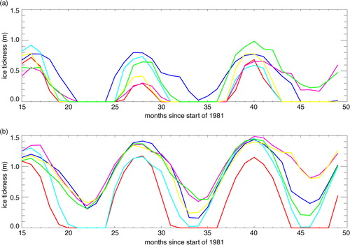
The 1981–1982 autumn–winter period, which formed the first 6 months of the experiments, is assumed to be a spin-up period and is not plotted on this or subsequent figures. In general, spin-up effects were not very noticeable, although there was some indication from the surface fluxes of an initial adjustment period over Lake Superior. Of all the locations examined, this lake has the largest depth, see Table 1. This initial transient may indicate that the lake initialisation currently coded in the MetUM reconfiguration, based on the temperature structure of the soil column, is inadequate for deep lakes. The database and/or approach of Kourzeneva et al. (2012) may be used in future to provide a better-conditioned initial state.

Figure 10 shows that in the original, unmodified experiment, Qinghai Lake persisted in a permanently frozen state, and Lake Sakakawea became permanently frozen for the third year of the experiment. This location was an isolated frozen gridbox, south-west of the main area of lake freezing in the Canadian Shield, see Fig. 6. The most successful modifications in ameliorating these unphysical states were the reduction of the lake-tile momentum roughness length and, especially, the change in the drag scheme. The combination of these two changes appears to be nonlinear, for example, the increase in length of the final non-frozen period in Fig. 10b. (Subsequent tests have shown that much of the improvement in ice behaviour can be obtained through a combination of the distributed-drag scheme and a reduction of roughness length of only one order of magnitude.)

The next section shows more general results from testing this optimum configuration.

4.3. Results from the optimum configuration

Month-by-month behaviour was examined more widely at the eight locations around the globe listed in Table 1 and plotted in Fig. 6. One of the main motivations of this point-based study was to examine behaviour around the Great Lakes, on account of the difference in the flux balance observed above, see Fig. 9. Thus, four of the locations were in the region of high lake fraction at the edge of the Canadian Shield. The southernmost of these was located on Lake Huron, corresponding to the point with the largest mean summer temperature perturbation of MetUM-FLake from the control run in Fig. 9.

The lake water-surface temperature (LWST) bi-monthly climatology produced by the ESA ARC-Lake project was also available for this study (MacCallum and Merchant, 2011), and it is used for additional comparison. MacCallum and Merchant (2012) indicate that, along with satellite data, FLake was also used in some aspects of the construction of this climatology.

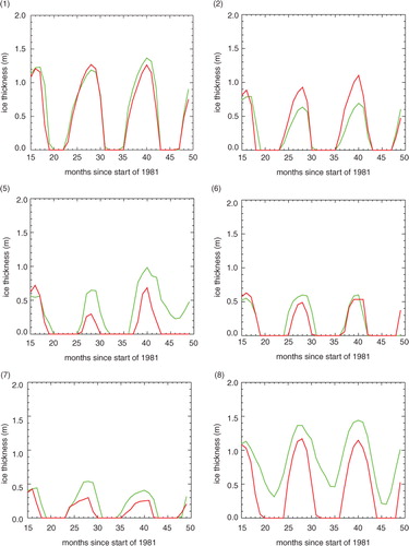
First, ice thickness is plotted in Fig. 11 for the six locations that had non-negligible winter ice thickness. The data for points 5 and 8 are the same as those plotted earlier, and they show the effect of the optimum configuration on reducing unphysical permanent ice cover. For the other locations, the effect on lake ice is more mixed, with point 2 having generally increased ice thickness, point 7 having generally reduced thickness, and points 1 and 6 showing little systematic difference. It would appear from this that the effect of the modifications is not merely to produce a general warming which reduces lake ice uniformly, but it is particularly evident at locations with high orography and orographic roughness, where the default configuration performs poorly. There is some indication, however, of a slight reduction in the duration of the frozen period with the modified configuration.

Fig. 11 Timeseries of monthly ice thickness at those test locations which formed lake ice, see Table 1 and Fig. 6. Green shows the original MetUM-FLake run. Red shows the MetUM-FLake run with modifications (B) and (D).

Monthly lake-tile temperature data are plotted for all locations in Fig. 12. As well as the default and modified MetUM-FLake runs, this figure shows the lake-tile temperature from the control MetUM run and the ARC-Lake climatology. It should be noted that the climatology does not provide surface temperatures for frozen lakes, but instead defaults to 0°C, which then indicates the frozen period. For this reason, and also to emphasise the differences in FLake output rather than those arising from the performance of the MetUM surface scheme over snow or ice, the plots are truncated to show mainly the non-frozen lake-tile temperatures. These temperatures are also more stable than those for the frozen state, and this is reflected in the smoothness of the plots at this timescale.

Fig. 12 Timeseries of monthly lake-tile surface temperature at the eight test locations, see Table 1 and Fig. 6. Black shows the control MetUM run. Green shows the original MetUM-FLake run. Red shows the MetUM-FLake run with modifications (B) and (D). Blue shows the ARC-Lake LWST climatology. Note that the climatology does not provide surface temperatures for frozen lakes, but instead defaults to 0°C, which then indicates the frozen period. No climatology data were available for location 5.

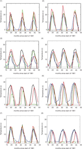
The temperature data in Fig. 12 indicate that the lake-tile surface temperature generally has a longer frozen period than the climatology. When not frozen, the peak in temperature is often shifted to a later time, compared to both the control MetUM run and the climatology. Such effects for lakes in the boreal zone were also observed by Kourzeneva et al. (2012). This shift in the timing of the annual temperature maximum appears to be an important factor in the large differences in summer mean temperatures, which were evident e.g. in Fig. 9. The data in Fig. 12 indicate that the difference in the maximum values at location 4 (Lake Huron) is about half the maximum difference in the mean summer temperatures computed in this region for the 10-yr comparison (Fig. 9d). Thus, the remainder of the difference in summer mean temperatures is attributable to the shift in peak temperature relative to the averaging window of June to August.

As with the lake ice, away from points 5 and 8 there appears to be little significant systematic difference evident in Fig. 12 between the default and modified MetUM-FLake runs in these timeseries. However, comparing the results of the original and modified MetUM-FLake configurations in a 10-yr climate run (see Fig. 13), reveals that the modified run produces a wintertime (December, January and February) cooling over large parts of the Northern Hemisphere land masses, which is not entirely beneficial in terms of model performance against climatology. In summer, the difference is mainly limited to the Canadian Shield, which is slightly warmer with the modified configuration. (Again, we assume that the differences in the Antarctic are attributable to circulation differences between the model runs.)

Fig. 13 Ten-year mean seasonal screen-temperature differences, computed as modified minus default MetUM-FLake configurations: (a) winter (December, January and February) and (b) summer (June, July and August).

5. Conclusion

We have presented a description of the coupling of FLake to the MetUM for weather and climate prediction. The MetUM system has been extended to include FLake prognostics and code-repository handling, and the FLake lake-depth database has been used to provide a lake-depth ancillary for global climate testing. However, full ancillary treatment of lake parameters and initialisation has yet to be incorporated into MetUM.

In tests of two standard model configurations, a high-resolution limited-area model of the UK and a global climate model, the overall impact of FLake has been found to be small at a statistical level, globally. However, we have shown an example of possible weather modification by an improved treatment of lakes at a local level.

Of equal interest is the behaviour of FLake upon coupling with MetUM. Examination of lake-ice thickness has revealed an unrealistic, annual or multi-annual persistence of lake ice at locations of high orographic roughness in the standard model configuration. Testing with a variety of modifications has revealed that a change in the MetUM sub-grid drag scheme, together with a change in the roughness length z ₀ of the lake tile, produces a more realistic annual cycle of freezing and melting at these points. This has been achieved without a general warming of the model, and it appears to target a particular feature of the model in locations of this type. This result is significant because FLake has been developed entirely outside MetUM, and it has been configured and tested against observational data. It is therefore a useful tool to gauge objectively the near-surface state of MetUM. Based on these tests, the distributed-drag scheme would appear to produce more realistic low-level winds than the orographic-roughness scheme in the standard configuration, albeit at the expense of increased wintertime screen-temperature bias with the current model physics settings. A possible further implication of this result is that the JULES surface exchange within MetUM may also be producing reduced fluxes in high orography, or may have been partly tuned to compensate for the wind error in such regions.

Finally, we hope to complete the implementation of FLake into standalone-JULES and MetUM in the near future, and thence to use it operationally in some MetUM configurations.

6. Acknowledgments

The authors thank Adrian Lock and Emma Fiedler for their help and advice.

References

- Balsamo G , Dutra E , Stepanenko V. M , Viterbo P , Miranda P. M. A , co-authors. Deriving an effective lake depth from satellite lake surface temperature data: a feasibility study with MODIS. Boreal Environ. Res. 2010; 15: 178–190.
- Best M , Beljaars A , Polcher J , Viterbo P . A proposed structure for coupling tiled surfaces with the planetary boundary layer. J. Hydrometeorol. 2004; 5(6): 1271–1278.
- Best M. J , Pryor M , Clark D. B , Rooney G. G , Essery R. L. H , co-authors . The Joint UK Land Environment Simulator (JULES), model description – part 1: energy and water fluxes. Geoscientific Model Dev. 2011; 4(3): 677–699.
- Brohan P , Kennedy J. J , Harris I , Tett S. F. B , Jones P. D . Uncertainty estimates in regional and global observed temperature changes: a new data set from 1850. J. Geophys. Res. Atmos. 2006; 111(D12):
- Clark D. B , Mercado L. M , Sitch S , Jones C. D , Gedney N , co-authors . The Joint UK Land Environment Simulator (JULES), model description – part 2: carbon fluxes and vegetation dynamics. Geoscientific Model Dev. 2011; 4(3): 701–722.
- Davies T , Cullen M. J. P , Malcolm A. J , Mawson M. H , Staniforth A , co-authors . A new dynamical core for the Met Office's global and regional modelling of the atmosphere. Q. J. Roy. Meteorol. Soc. 2005; 131(608): 1759–1782.
- Fox S , Wilson D , Lewis W . Neon: the UK Met Office electro-optic tactical decision aid-current and future capability. Proc. Optics in Atmospheric Propagation and Adaptive Systems XIII, 782805. 2010
- Frauenfeld O. W , Zhang T , McCreight J. L . Northern hemisphere freezing/thawing index variations over the twentieth century. Int. J. Climatol. 2007; 27(1): 47–63.
- Fuller R. M , Groom G. B , Jones A. R . The land cover map of great Britain: an automated classification of Landsat Thematic Mapper data. Photogramm. Eng. Remote Sensing. 1994; 60(5): 553–562.
- George D. G , Taylor A. H . UK lake plankton and the Gulf Stream. Nature. 1995; 378: 139.
- Kourzeneva E . External data for lake parameterization in Numerical Weather Prediction and climate modeling. Boreal Environ. Res. 2010; 15: 165–177.
- Kourzeneva E , Martin E , Batrak Y , Le Moigne P . Climate data for parameterisation of lakes in numerical weather prediction models. Tellus A. 2012; 64
- Kourzeneva K , Braslavsky D , Gollvik S . Lake model FLake, coupling with atmospheric model: first steps. 4th SRNWP/HIRLAM Workshop on Surface Processes and Assimilation of Surface Variables jointly with HIRLAM Workshop on Turbulence. 2005; SMHI, Norrkoping, Sweden. 43–54.
- Lindvall J , Svensson G , Hannay C . Evaluation of near-surface parameters in the two versions of the atmospheric model in CESM1 using flux station observations. J. Clim. 2013; 26(1): 26–44.
- Lofgren B. M . Simulated effects of idealized Laurentian Great Lakes on regional and large-scale climate. J. Clim. 1997; 10(11): 2847–2858.
- Loveland T. R , Reed B. C , Brown J. F , Ohlen D. O , Zhu Z , co-authors . Development of a global land cover characteristics database and IGBP DISCover from 1 km AVHRR data. Int. J. Remote Sens. 2000; 21(6–7): 1303–1330.
- MacCallum S. N , Merchant C. J . ARC-Lake v1.1, 1995–2009. [dataset]. 2011. Online at: http://www.geos.ed.ac.uk/arclake/ .
- MacCallum S. N , Merchant C. J . Surface water temperature observations of large lakes by optimal estimation. Can. J. Remote Sens. 2012; 38(1): 25–45.
- Mironov D , Heise E , Kourzeneva E , Ritter B , Schneider N , co-authors A . Implementation of the lake parameterisation scheme FLake into the numerical weather prediction model COSMO. Boreal Environ. Res. 2010; 15: 218–230.
- Mironov D. V . Parameterization of Lakes in Numerical Weather Prediction. Description of a Lake Model.
- Potes M , Costa M. J , da Silva J. C. B , Silva A. M , Morais M . Remote sensing of water quality parameters over Alqueva Reservoir in the south of Portugal. Int. J. Remote Sens. 2011; 32(12): 3373–3388.
- Potes M , Costa M. J , Salgado R . Satellite remote sensing of water turbidity in Alqueva reservoir and implications on lake modelling. Hydrol. Earth Syst. Sci. 2012; 16(6): 1623–1633.
- Rooney G. G , Jones I. D . Coupling the 1-D lake model FLake to the community land-surface model JULES. Boreal Environ. Res. 2010; 15: 501–512.
- Sobek S , Nisell J , Folster J . Predicting the depth and volume of lakes from map-derived parameters. Inland Waters. 2011; 1(3): 177–184.
- Subin Z. M , Riley W. J , Mironov D . An improved lake model for climate simulations: model structure, evaluation, and sensitivity analyses in CESM1. J. Adv. Model. Earth Syst. 2012; 4(1):
- Tang Y , Lean H. W , Bornemann J . The benefits of the Met Office variable resolution NWP model for forecasting convection. Meteorol. Appl. 2012
- Walters D. N , Williams K. D , Boutle I. A , Bushell A. C , Edwards J. M , co-authors . The Met Office Unified Model global atmosphere 4.0 and JULES Global Land 4.0 configurations. Geoscientific Model Development Discussions. 2013; 6: 2813–2881.
- Williamson C. E , Saros J. E , Vincent W. F , Smol J. P . Lakes and reservoirs as sentinels, integrators, and regulators of climate change, Limnol. Oceanogr. 2009; 54(6, part 2): 2273–2282.
- Wood N , Brown A. R , Hewer F. E . Parametrizing the effects of orography on the boundary layer: an alternative to effective roughness lengths. Q. J. Roy. Meteorol. Soc. 2001; 127(573): 759–777.
- Wood N , Mason P . The pressure force induced by neutral, turbulent flow over hills. Q. J. Roy. Meteorol. Soc. 1993; 119(514): 1233–1267.
- Zilitinkevich S. S . Turbulent Penetrative Convection. 1991; Avebury Technical, The Academic Publishing Group, Aldershot, England.