A response in the ENSO cycle to an extratropical forcing mechanism during the El Niño to La Niña transition

Abstract

Current El Niño-Southern oscillation (ENSO) theory emphasizes that the forcing that drives the cycle mainly exists within tropical regions. However, these ideas are quite limited in explaining completely the occurrence of ENSO. Here, we examine whether extratropical forcing can affect ENSO cycle, specifically the transition from El Niño to La Niña. Although dispersion of the Okhotsk-Japan (OKJ) atmospheric wave train across the mid-latitude North Pacific during June terminates in the subtropics, the associated regime of southward surface wind anomalies could reach Eastern Equatorial Pacific (EEP). The OKJ wave train plays a substantial role in generating a similar underlying sea surface temperature (SST) wave train through a barotropic process in air–sea interactions and after September, it is negatively correlated strongly with the SST around EEP. Strong OKJ propagation in the positive (negative) phase during June is more (less) significantly associated with a subsequent La Niña (El Niño) episode that is matured after October. Negative SST anomalies at the southern end of the SST wave train with strong overlying OKJ propagation in the positive phase during June and the associated southward surface wind anomalies retained its strength by the further infusion of energy and gradual southward displacement joining the negative SST anomalies around EEP after the October when La Niña usually matured in-situ. Strong OKJ propagation in the positive phase during June tends to occur during a quick summer and fall transition period from El Niño to La Niña. This study strongly suggests that extratropical forcing plays an ignored role in affecting ENSO cycle especially in the formation of La Niña, which was not included in current ENSO theory.

• Rossby wave
• ENSO cycle
• air–sea interaction

To access the supplementary material to this article, please see Supplementary files under Article Tools online.

1. Introduction

The El Niño-Southern oscillation (ENSO) cycle predicates the alternating occurrence of El Niño and Anti-El Niño (La Niña) with a period of about 2–7 years (McPhaden et al., 2006), and which deeply affects human life. Since an atmospheric bridge linking the ENSO with tropical sea surface temperature (SST) anomalies was introduced by Bjerknes (1966, 1969), the understanding of the ENSO mechanism has improved rapidly. Subsequently, evidence (Wytrki, 1975) has shown that almost all of the occurrences of El Niño are closely associated with a sudden weakness of the trade winds and the variation of the thermocline from the west to the east tropical Pacific is a substantial sign of ENSO event onset.

The delayed-oscillator model is currently one of the widely acknowledged theories for explaining the ENSO cycle (Battisti, 1988; Schopf and Suarez, 1988; Battisti and Hirst, 1989; Tziperman et al., 1994). This theory declares that wind stress from the trade winds provides a positive ‘Bjerknes feedback’ on East Pacific SST anomalies (SSTA), while equatorially trapped waves in the upper ocean that propagate across the Pacific and reflect at the boundaries affords a delayed restoring force. Thus, a build-up of the heat content in the Western Pacific is a forerunner of El Niño and the build-down of the heat content in the region plays the opposite role. However, all ENSO theories were limited to discussing the evolution of these elements within tropical regions.

Chiang and Vimont (2004) found that the Intertropical Convergence Zone in the Pacific Region can be displaced toward the warm hemisphere in an analogous manner to that in the Atlantic. They called this phenomenon the Pacific Meridional Mode (PMM) and found that, as in the Atlantic, this phenomenon originated in the trade wind belt. Zhang et al. (2009) found that the PMM emerges during the Northern Hemisphere spring and occasionally links to the ENSO phenomena. Their study also demonstrated that the PMM connection to the ENSO is confined to tropical region; however, Chiang and Vimont (2004) suggest that the PMM may provide a bridge to connect the extratropics to the tropics.

Thus, it cannot be denied that impacts from factors originating in the extratropical regions on the ENSO cycle could potentially exist since the exchange of the energy between the tropical and the extratropical regions occurs all the time. The major problem is that such evidence regarding the extratropical influences especially from the atmosphere is extremely hard to obtain. It is well known that atmospheric eddies rarely travel from extratropical to tropical regions due to the differing basic flow in the two regions. Thus, the extratropical atmospheric impacts on ENSO may be more easily hidden by either highly chaotic effects occurring in the climate system or other random factors which cannot be predicted compared with the tropical influences. On the other hand, current ENSO theory is not perfect, as it fails to explain adequately the onset or termination of El Niño (McPhaden, 1999). One of the major problems is that the equatorial oceanic waves as dynamic indices for measuring ENSO cycle evolve too fast in a coupled atmosphere–ocean model compared to the observed ENSO time-scale (Deser et al., 2006). Thus, identifying an extratropical impact on the decay or the transition (warm to cold or cold to warm) of the ENSO cycle would be helpful to improve the theory regarding its evolution, which is the primary purpose of this study. Such a mechanism was suggested by earlier studies. Finally, in order to better understand the role of such an extratropical forcing mechanism, we provided a simple schematic to summarize the major result found here.

2. Data

There was an inter-decadal change in the character East Asia summer monsoon between the periods before and after 1963, as pointed by Wang and Lupo (2009). They proposed that this change might be due to the sparse data available over the Pacific. Consequently, this study does not include the data from the period before 1963. The National Centers for Environmental Prediction (NCEP)/National Center for Atmospheric Research global atmospheric reanalysis dataset is the primary dataset used in this study (Kalnay et al., 1996). Specifically, the monthly (1963–2011) 500-hPa geopotential heights (Z500) on a 2.5° latitude/longitude grid were used here. To provide a convenient benchmark, the 1981–2010 height climatology of 500 hPa is used for generating the anomalies and long-term mean plots, which can be found at: http://www.esrl.noaa.gov/psd/cgi-bin/data/composites/printpage.pl from the Earth System Research Laboratory. The National Oceanic and Atmospheric Administration Extended Reconstructed monthly SST V3b on a 2° latitude/longitude grid from 1963 to 2011 was used.

3. ENSO occurrences and the OKJ wave train

3.1. An asymmetric transition of ENSO

Historically, El Niño (warm) and La Niña (cold) events often appear to follow one after another. Both of them tend to mature near the end of a calendar year (Rasmusson and Carpenter, 1982). However, they may not occur with roughly the same time interval in between them. Table 1 shows the years when the warm (cold) episodes matured in a minimum of five consecutive overlapping seasons including October to the following February, in which±0.5K for the Oceanic Niño Index was the threshold for determining warm/cold events. The definition for the ENSO events was provided by the Climate Prediction Center, and can be found at: http://www.cpc.ncep.noaa.gov/products/analysis_monitoring/ensostuff/ensoyears.shtml. Although the number of warm and cold events was almost the same (Table 1), the occurrence of a cold event following a warm one in the following year (quick succession) was far more common than the opposite case. Ten pairs belong to the former category, i.e. 1963–1964, 1969–1970, 1972–1973, 1982–1983, 1987–1988, 1994–1995, 1997–1998, 2004–2005, 2006–2007 and 2009–2010, but there are only five pairs for the latter, i.e. 1964–1965, 1971–1972, 1975–1976, 2005–2006 and 2008–2009, respectively. Thus, a quick transition period from El Niño to La Niña tends to occur in most of the cases where the phases appeared back-to-back. This asymmetric occurrence in the transition between the warm/cold events implies that the air–sea coupled climate system itself possesses the tendency to quickly eliminate the El Niño conditions. This would be related to the restoring force that tends to bring the El Niño state back to equilibrium. This was discussed in the delayed-oscillator theory. A forcing originating from extratropical regions might be an important source of this restoration since a large quantity of heat must be exchanged between north and south regions to keep the balance in a rather conservative global climate system.

Table 1. Warm and cold years when the episodes matured after October

Warm events	Cold events
1963	1964
1965	1970
1968	1971
1969	1973
1972	1974
1976	1975
1977	1983
1982	1984
1986	1988
1987	1995
1991	1998
1994	1999
1997	2000
2002	2005
2004	2007
2006	2008
2009	2010
2011

3.2. The OKJ wave train

The SST tends to respond to an equivalent-barotropic low-frequency atmospheric anomaly as a linear process and there is a positive feedback of large-scale eddies, reinforced by high frequency eddies (or an eddy mediated process), on the ocean mixed layer temperature (Kushnir et al., 2002). The air–sea interaction results in a warm (cold) SST centre with an overlying high (low) height centre up to approximately middle troposphere. Although we cannot show the movement of the sea surface water here, the in-situ sea current would have a similar circulation forced by the overlying flow without other impacts. Note that the SST anomalies do not always represent changes in ocean current; see section 7 for a detailed footnote.

On the other hand, atmospheric Rossby waves acting as a transmitter of energy exist almost everywhere. The energy dispersion of the Rossby wave is able to intensify or weaken eddies downstream. The quasi-stationary atmospheric Rossby wave propagation, which is associated with the development of the Okhotsk High, could play a role in forming a SST wave train (SWT) through an air–sea interaction process in the extratropical Pacific in early summer (Wang and Lupo, 2009). This Rossby wave is called the Okhotsk-Japan (OKJ) wave, which may be largely enhanced by the preceding El Niño event (Wang and Lupo, 2009). The primary question here is: if El Niño can impact the circulation over extratropical regions in terms of the Rossby wave propagation, why can't the ENSO receive a feedback from the extratropics in return? However, extratropical Rossby waves cannot propagate from extratropical regions into the equatorial regions directly because according to Rossby wave ray theory, Rossby wave dispersion in the westerlies is blocked as it meets the easterlies over subtropical regions (Hoskins and Karoly, 1981). Rossby wave trains in lower latitudes tend to have smaller amplitudes than those in higher latitudes. It is probably impossible that Rossby waves from extratropical regions directly cause variations in the circulations over the equator so as to affect the equatorial SST by the barotropic air–sea interaction without the westerlies extending to the equator. However, what role the SWT can play within the extratropical region pointing toward the equator (Wang and Lupo, 2009) still challenges our imagination. Since extratropical Rossby waves have little direct impact on the tropics, this was the reason why the signal in SWT was examined here.

In order to investigate if the extratropical forcing impacts the tropics, first we introduce the OKJ index in June (OKJ–JUN), which is simply a measurement of amplitude of the OKJ propagation during June. This index was derived using the methods of Wallace and Gutzler (1981) and described in earlier research papers (e.g. Wang, 1992), but a detailed description of the index can be found in Wang et al. (2013) in which other derivations by using normal and rotated empirical orthogonal functions were investigated also. The OKJ index is designed as follows:

In eq. (1 ), Z^* denoted the normalized height anomalies at 500 hPa. A positive index is indicative of anomalously high height around the Okhotsk Sea, and low heights around the Lake Baikal and the Pacific Ocean east of Japan, while a negative index indicates the opposite sense. We assigned the first grid point (57.5°N, 137.5°E) twice the weight of the other two grid points to make the sum of the weight equal to zero. This assignment also emphasized the importance of the height change around the Okhotsk Sea since OKJ wave propagation in the positive phase during June (OKJ-POS) is associated with the Okhotsk High, which plays a role in maintaining persistent monsoon rainfall in China (Wang, 1992). In this sense, OKJ propagation in the negative phase in June tends to occur rarely.

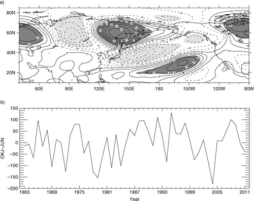
Figure 1a shows the correlation between the index and Z500 and Fig. 1b shows year-to-year fluctuations in the index. We can see the correlation centres extending from European regions in high latitudes to the subtropical Pacific sea areas in Fig. 1a, which coincides with the OKJ pattern (Wang, 1992; Wang et al., 2007). This is a late-spring and summer teleconnection pattern that is similar to those such as the Pacific North America pattern (e.g. Wallace and Gutzler, 1981; Lupo and Bosart, 1999). Except for the normal OKJ action centres, an additionally significant positive correlation centre (30°N, 155°W) and a less significant negative one (15°N, 142.5°W) that penetrated into subtropical Eastern Pacific can also be found (Fig. 1a). These additional correlation centres, which were not widely recognized before, imply that air–sea interactions might occur over the subtropical region that is close to the areas where warm/cold events are usually identified. Note that high values of the OKJ–JUN are roughly associated with a previously strong El Niño event, e.g. that in 1997–1998 (coinciding with the result of Wang and Lupo, 2009).¹

Fig. 1 The correlation coefficient between the OKJ–JUN and Z500 in (a) June and (b) the evolution of the OKJ–JUN from 1963 to 2011. Shaded areas in (a) indicated the regions over the 95% confidence level. The contour interval is 0.1.

4. The correlation between OKJ wave train and SST over the North Pacific

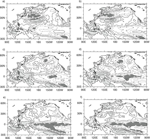
Figure 2a–f showed the correlations between the OKJ–JUN and SST in June, and the following July, August, September, October and November, respectively. Significant positive, negative and positive correlation areas were located around the Okhotsk Sea, the Kuroshio Extension and the area to the south of the Kuroshio Extension, respectively (Fig. 2a), which suggests a clear wave train structure. The correlation centres in the extratropical Pacific in Fig. 2a roughly coincided with those in Fig. 1a. This pattern significantly persisted through the next month (Fig. 2b). On the other hand, a significant negative correlation area in Eastern Equatorial Pacific (EEP) emerged in Fig. 2c and then became strong in Fig. 2d–f. The correlation implied that the strong OKJ-POS occurring during June tends to be associated with an EEP cooling by the end of the year and vice versa. Since both La Niña and El Niño normally mature in the boreal winter, the preceding OKJ propagation may be linked with the cool ENSO events forming.

Fig. 2 The correlation coefficient between the OKJ–JUN and SST during (a) June, (b) July, (c) August, (d) September, (e) October, (f) November, from 1963 to 2011. Shaded areas indicated the regions over the 95% confidence level. The contour interval is 0.1.

We divided the values of OKJ–JUN into three intensity levels, i.e. Level 1: larger than 11 units; Level 2: −10 units to +10 units; Level 3: lower than −11 units (Table 2), in order to further check the relationship between OKJ–JUN and the warm/cold events listed in Table 1. The Level 2 events in Table 2 show that the moderate index values are relatively infrequent. The result from Table 2 shows a preponderance for the occurrence of rapid transition from warm to cold ENSO events. The percentage between cold (warm) events in Level 1 (Level 3) and those in Level 1 and 3 is 11/14 (9/15) without the inclusion of events occurring in Level 2, in which there are two warm and four cold events. In spite of the limited number of samples, we have performed a Chi-square (χ²) test for the cold and warm events in Level 1 and Level 3 columns of OKJ index without counting the neutral events.² The occurrences of cold (warm) events in Level 1 (Level 3) rejected the null hypothesis at the 0.05 (0.10) significance level. In addition, the percentage of the events with single asterisk in Level 1 is 7/7 whereas that with double asterisks in Level 3 is 3/4 when limiting the count to Levels 1 and 3. These results suggested that the strong OKJ-POS tends to be followed more frequently by a cold event than the negative phase OKJ propagation during June with a subsequent warm event. Furthermore, the strong OKJ-POS tends to be much more often associated with a preceding warm event followed immediately by a cold event, rather than the opposite situation. Thus, the strong OKJ-POS Index tends to appear during the quick summer and fall transition period from El Niño to La Niña. The OKJ-POS accompanying the development of the Okhotsk High appeared to be much more robust than the OKJ propagation in the negative phase in June because the Okhotsk High is normally strong in June (Wang et al., 2007). This can be further confirmed by the OKJ–JUN values in Table 2, i.e. the years in Level 1 were more numerous than those in Level 3.

Table 2. The years with the OKJ–JUN values for the three intensity levels of the index from 1963 to 2011

Level 1: OKJ–JUN≥11		Level 2: OKJ–JUN ≤ ∣10∣		Level 3: OKJ–JUN≤− 11
Year	OKJ–JUN	Year	OKJ–JUN	Year	OKJ–JUN
1966	96.7	1964*	−6.5	1963	−14.4
1968	55.2	1971	−0.4	1965**	−65.9
1970*	13.6	1977	6.6	1967	−15.5
1973*	34.3	1985	−9.2	1969	−104.6
1974	80.3	2005*	8.7	1972**	−126.1
1975	79.2	2006**	7.1	1976**	−45.8
1981	23.4	2010*	−3.0	1978	−127.4
1983*	35.3	1979	−153.4
1986	59.2	1980	−62.0
1987	30.5	1982	−109.9
1988*	94.0	1984	−100.8
1989	96.6	1991	−13.7
1990	48.2	1994	−83.0
1992	110.4	2000	−75.0
1993	30.8	2001	−41.3
1995*	130.5	2003	−80.5
1996	40.8	2004	−179.9
1997	37.4	2011	−40.1
1998*	85.8
1999	12.0
2002	12.3
2007*	51.5
2008	100.5
2009**	77.5

Italic and bold digits indicate warm and cold years, respectively, listed in Table 1. Single (double) asterisks show the cold (warm) years that follow warm (cold) years immediately.

5. Evolution of the observational elements

5.1. Composite maps

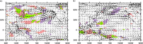
Figure 3(a–d) shows the composite of Z500 and horizontal wave activity flux (HWAF) with the OKJ–JUN to be higher than 50 units and lower than −50 units for the months of June and November, respectively. Figure 4(a–d) shows a similar composite except for the anomalies of the Z500 and the SST. For brevity, we omitted the figures (Supplementary file) that connected with Figs. 3 and 4 from July to October. The HWAF was used to indicate the direction and magnitude of stationary wave propagation (Plumb, 1985; Wang and Yasunari, 1994; Wang et al., 2007). The south-eastward HWAF (SE-HWAF) associated with a large Okhotsk High strongly propagated from the upstream Okhotsk Sea region extending into the subtropical Pacific during June (Fig. 3a). Large fluxes could be found even around 22.5°N, 140°W, indicating that the in-situ circulation would be enhanced by OKJ-POS environment. At the same time, narrow strips of significantly positive, negative and positive SSTA tilted northwest–southeast appeared with a wave train-like structure over the extratropical Northern Pacific (Fig. 4a). Note that a significant high (low) SSTA centre was basically covered by an overlying significant high (low) Z500 anomaly (Z500A) centre in spite of a minor phase drift. According to the quasi-geostrophic approximation, an anomalous horizontal wind that roughly parallels the anomalous height contour line tends to follow an anomalously cyclonic (anticyclonic) rotation around a negative (positive) Z500A centre over extratropical regions. Since the SWT was generated by the OKJ propagation through the process of quasi-barotropic air–sea interaction (e.g. Kushnir et al., 2002), an anomalous sea current associated with the SWT should move horizontally similar to the overlying air flow. The centre positions in Fig. 4a roughly coincided with those in Fig. 2a. Note that significantly southward (northerly) surface wind anomalies (SSWA) generated by the anticyclonic rotation from the east side of an anomalously anticyclonic centre (30°N, 155°W, Fig. 5a) extended all the way from the extratropical region down to the EEP. Because there should be an anomalously oceanic anticyclonic centre forced by the overlying the atmospheric one, a similar southward sea surface current anomalies from the east side of the oceanic eddy is foreseeable. This was the impact of the OKJ propagation also (Kushnir et al., 2002; Wang and Lupo, 2009). Note that the surface anticyclonic air flow centre was located only near a positive SSTA centre (37.5°N, 150°W, Fig. 4a) at the south-eastern end of the SWT. Another notable feature is that the easterly anomalies along the equator dominated at all times (Fig. 5a and 5b; Supplementary file), which coincides with the explanation for La Niña forming in the original ENSO theory. The SWT pattern roughly remained through July and the major part of the wave train weakened moving to the northeast Pacific during August when no strong SE-HWAF appeared (Supplementary file). The SWT in the east was significantly enhanced by the accompanying and stronger overlying SE-HWAF during September (Supplementary file). The initial SWT pattern less significantly reappeared in November when an overlying strong SE-HWAF dominated again (Fig. 3b and 4b). Nonetheless, although the negative SSTA had weakly existed in the EEP since June, the strength and the scope of it continued to expand in the following months. Additionally, the La Niña, which is marked by the negative SSTA in the EEP, had significantly matured since September. In fact, the significantly negative SSTA with a strong centre near the equator extending to about 20°N began to appear in August (Supplementary file). Note that this La Niña SST emerged just two months after the establishment of the OKJ wave train. The negative SSTA developed in a wide belt during the mature phase of La Niña (e.g. Fig. 4b). The development of negative SSTA in the EEP can simply be seen as a consequence of Table 2. The data going into the composite has a preference for a developing cold ENSO event. This part provided major evidences for the mechanism and its evolution that is depicted in a schematic (Fig. 10) in Section 7.

Fig. 3 The composite of Z500 and HWAF (unit: m² s⁻²) for the years: 1966, 1968, 1974, 1975, 1986, 1988, 1989, 1992, 1995, 1998, 2007, 2008, 2009 for (a) June and (b) November, and for the years 1965, 1969, 1972, 1978, 1979, 1980, 1982, 1984, 1994, 2000, 2003, 2004 for (c) June and (d) November. The blank area between 10°S and 10°N indicates the HWAF near zero. The contour interval is 40 gpm.

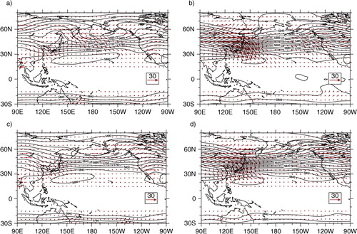
Fig. 4 As in Fig. 3, except for the composite of SSTA and Z500A. Thin contour line indicated SSTA (interval 0.1 K) and thick lines show the contour of the Z500A (interval: 10 gpm). Areas with purple (pink) colour indicated the regions where the difference in Z500 anomalies (SSTA) between high and low OKJ composite were statistically significant at 95% confidence level by t-test. Areas with green colour indicated the overlapping regions for the significant SSTA and Z500 anomalies.

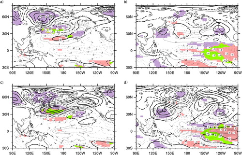
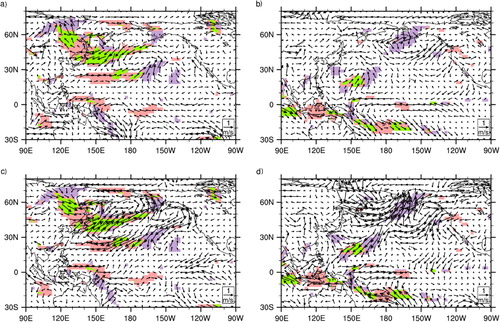
Fig. 5 As in Fig. 3, except for the anomalies of the surface wind vector (unit: ms⁻¹). Areas with purple (pink) colour indicated the regions where the difference in meridional (zonal) surface wind anomalies between high and low OKJ composite were statistically significant at 95% confidence level by t-test. Areas with green colour indicated the overlapping regions for the significant meridional and zonal wind surface anomalies.

On the contrary, Fig. 4c–d outwardly appeared to display the opposite signs when compared with Fig. 4a–b. However, the positive SSTA in the EEP, which represents the El Niño phenomenon, appeared in a much narrower belt (mainly within 10°N–10°S) than that in Fig. 4a–b. Although the atmospheric forcing could similarly produce SWT-like structures in extratropical regions (Fig. 4c), the SE-HWAF (Fig. 3c) that measures the OKJ propagation in the negative phase was weaker especially during June than that shown in Fig. 3a. In addition, the negative SSTA covered most of oceanic areas to the north of the positive SSTA in the EEP (Fig. 4d). There was no SSWA extending into the EEP in June. Note that although north-easterly surface wind anomalies appeared in the region of 0–10°N, 100–160°W, more significant westerly surface wind anomalies dominated from 130°E to 160°W along the equator during November when a strong El Niño SSTA covered the EEP (Fig. 4d and 5d). This sign coincides strongly with the current explanation for El Niño formation.

5.2. The case of the 1998 transition

As the composite showed in first subsection, the SWT caused by atmospheric forcing in the extratropical regions was associated with the negative SSTA around the EEP after autumn when mature phase of La Niña tends to occur. Here, we investigate further this phenomenon involving the El Niño event of 1997–1998 that was the one of the strongest on record. The quick transition from El Niño to La Niña occurred during the summer of 1998 (Table 2). In addition, the OKJ–JUN reached 85.8 units in 1998 and belongs among the strongest OKJ-POS values.

The strong SE-HWAF accompanying the development of the Okhotsk High widely dominated over the mid-latitudes of the north Pacific during June of 1998 (Fig. 6a). Compared with the composite (Fig. 4a), the anomalous centres of the OKJ-like wave train were distributed over the farther north-eastward ocean areas (Fig. 7a). The strong SE-HWAF penetrated into the subtropics to about 20°N, 110°W (Fig. 6a), which implies the extending of an area of the impact of the OKJ-like propagation on the SSTs. The oceanic region with the SWT was only covered by the strong overlying SE-HWAF. Afterward, the strong SE-HWAF did not occur until November (Fig. 6b; Supplementary file). However, the SWT roughly persisted in its position from July to September (Supplementary file) and largely shifted its phase southward by November. The southern end of the SWT was connected with the negative SSTA around the EEP after October (Fig. 7b; Supplementary file) when the La Niña matured completely. Note that the negative SSTA was mainly located on the northern side of the equator in autumn (Fig. 7b; Supplementary file). On the other hand, the SSWA was strongly forced outward from the east side of the anticyclonic surface wind centre (45°N, 150°W, Fig. 8a) and extended into the EEP during June also. The anticyclonic surface wind centre shifted southward to about 30°N until November (Fig. 8b; Supplementary file) and a strong SSWA extending into the EEP existed during the entire time. Thus, the case study here showed strong similarities to the composite analysis.

Fig. 6 As in Fig. 3, except for (a) June and (b) November 1998.

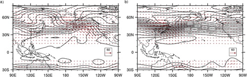
Fig. 7 As in Fig. 4, except for (a) June and (b) November 1998. The contour interval for the Z500A is 20 gpm and that for SSTA is 0.3 K.

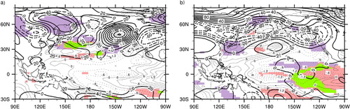
Fig. 8 As in Fig. 5 except for (a) June and (b) November 1998.

6. Summary

Based on the statistical and composite analyses above, the results of this study are summarized below:

1. The sphere of the influence of the OKJ-like atmospheric wave train or teleconnection during June could be extended from East Asia across the mid-latitude north Pacific reaching to about 15°N, 142.5°W which is near the equatorial region of the Eastern Pacific (the less significant correlation centre as shown in Fig. 1a). The atmospheric wave train basically accompanies an underlying SWT over the extratropical regions.

2. The OKJ–JUN is strongly negatively correlated with the SST around the EEP especially within those regions to the east of the International Date Line after September.

3. The percentage of the occurrences of La Niña events accompanied by a previously strong OKJ-POS index is much larger than that of an El Niño event with a previously strong OKJ propagation in the negative phase during June. Thus, for a majority of rapid ENSO transition cases, the La Niña events succeed the El Niño events in association with a strong OKJ-POS Index, but not vice versa.

4. An additional positive height anomaly centre over northeast Pacific (APHAC), which is associated with the OKJ-POS, tends to generate an SSWA that approaches the EEP.

5. The SWT created by a strong OKJ-POS could persist for about 2 months without succeeding supplementary SE-HWAF. Any kind of upstream SE-HWAF could enhance the SWT and adjust some of its position or extent. The southern end of the SWT associated with the SSWA joined the strong negative SSTA located around the EEP after October or November when La Niña usually matured. On the other hand, although the similar SWT in the opposite phase can be produced by strong OKJ propagation in the negative phase in June, no positive SSTA at the southern end of the SWT joined the positive SSTA around the EEP.

7. Discussions

Thus, the results demonstrate a clear mid-latitude genesis region for the proposed forcing mechanism on El Niño here. Such a mechanism was suggested in earlier studies (e.g. Chiang and Vimont, 2004), but not described until this study. Additionally, this mechanism is clearly not the PMM as the PMM is generated in the spring and in the trade wind area. However, in light of other studies, the PMM could serve as a bridge for the proposed mechanism here to interact with El Niño. Alternately, this mechanism could merge with the PMM during its evolution and the PMM is part of this proposed mechanism.

There are two questions generated here by the above results: (1) why is June important in identifying the impact of the atmospheric forcing on the maturing La Niña 3–5 months later? (2) How does the atmospheric forcing in the extratropical region through the generated SWT affect the SSTA in the EEP?

The answer for (1) is due to the large thermal contrast between the continent and the Western Pacific in mid- to high latitudes, that is formed annually typically by, and into, June such that the OKJ-POS index accompanying the development of the blocked Okhotsk High tends to occur (Wang, 1992). The preceding El Niño may further enhance the OKJ-POS associated with a strong Okhotsk High (Wang and Lupo, 2009). The SWT associated with the SE-HWAF may exist prior to June (Supplementary file). However, there is no relatively stable teleconnection pattern in the region that can organize the SWT as effectively during other seasons such as that which normally appears during June of a decaying El Niño event. The initially extratropical forcing during June appears more important in decreasing SSTs in the subsequent EEP.

On the other hand, the evolution of the oceanic circulation is much slower than that of the atmospheric circulation. The oceanic circulation of the SWT may persist in its strength for about 1–2 months or possibly more without the additional supplement of energy whereas the atmospheric wave train cannot. The SWT that was caused by an overlying eddy can be regarded as a kind of oceanic wave train that may have a similarly anomalous flow to the overlying air flow (e.g. Fig. 5a). The SWT would be able to act as either a stationary Rossby wave or a phase propagating planetary wave by inheriting the feature of the atmospheric wave train. The APHAC attached in the southern end of the OKJ-POS is able to cause underlying warm water as discussed above. Meanwhile, it would be a key component in the system for causing a negative SSTA in the EEP. The SSWA could be produced by the anticyclonic rotation on the eastern side of APHAC.³ According to Ekman theory, the sea surface current tends to be at a systematic deviation of about 45° to the surface wind in the direction of higher pressure in middle latitudes (Peixoto and Oort, 1992), which suggests that an atmospheric anticyclonic eddy could generate a similar oceanic anticyclonic eddy below. Similar to the SSWA escaping out from the atmospheric eddy, there must be similar southward surface current anomalies (SSCA) flowing out from the oceanic one as well. Note that the SSWA could extend to the south of 20°N where the Coriolis force has been largely reduced. In this case, the surface Ekman transport of the SSWA that is superposed on the SSCA forced by the oceanic eddy would be mainly southward but with a slightly westward component. Suppose the SWT is also acting as an oceanic Rossby-like wave that is further enhanced by the strong upstream SE-HWAF, and the continuously generated SSCA can gradually push the cooler waters from extratropical region into the EEP where the sea surface height is decreasing normally with a large poleward SST gradient (Fig. 9). However, the cooling process in this study may include some transition of the ENSO itself also, since the original ENSO theory that explains the cooling mechanism cannot be ignored. The significant negative SSTA in the EEP could occur in August two months after OKJ-POS establishment and might be a sign. The southward advection of SST from the southern end of the APHAC (e.g. ~20°N) to the equator would be estimated to take about 2 months if the advection speed is remaining ~0.5 ms⁻¹. In fact, the SSCA occurring in June would be able to arrive at 15°N or further south if considering the position that the SSWA reached (Fig. 5a). In addition, the SSWA that joined the EEP may play a role in enhancing the trade wind that is crucial to forming La Niña in the original ENSO theory. The slightly westward bias of the SSCA caused by Coriolis force and other damping factors might further slowdown the cooling process that would mainly function to the west of 140°W (Fig. 5a). Suppose the APHAC remains for 2 months (e.g. June and July if following the wave train pattern in Fig. 2a–b), large quantities of cold water would be transported into EEP until October or November when La Niña usually matures. It is highly plausible that this cooling process could accelerate the La Niña formation progress. The composites provide strong evidence for this point, in which the negative SSTA belt in the EEP after autumn is much more widely distributed along the equator than the positive SSTA (see Fig. 4b,d). However, how soon (especially the indirect) the influence of the OKJ wave train can reach the EEP remains a mystery due to the complex air–sea interactions as discussed here.

Fig. 9 The SSTs during (a) June, and (b) November averaged from 1963 to 2011. The contour interval is 1°C.

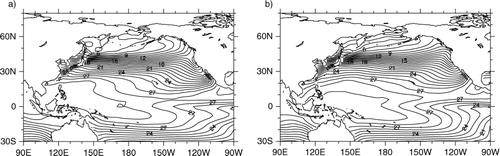
On average, the poleward SST gradient appeared much larger in the EEP than that in the western equatorial Pacific during June and November (Fig. 9). Thus, it is reasonable to assume that the negative SSTA in the western equatorial Pacific is caused mainly by the upwelling water as in the delayed-oscillator described due to the in-situ broad warm water area. However, the SSTA in the EEP is not only caused by in-situ upwelling water, but is also easily affected by cold water transported from higher latitudes due to the in-situ narrow warm water area. This is the reason why the extratropical forcing proposed here cannot support the formation of El Niño. Contrarily, the positive SSTA in the western equatorial Pacific or the EEP could more easily affect SSTs or weather over extratropical regions, as shown by many studies (e.g. Simmons et al., 1983). On the other hand, this study only focuses on the forcing from the Northern Hemisphere, and may not be sufficient to explain entirely the transition to La Niña, although the case studied here from 1998 suggests the point. The equator-ward HWAF in the Southern Hemisphere during June was also found in the composites (Fig. 3a). The cold water from higher latitudes of the Southern Hemisphere side would be easily pushed into the EEP as well. The forcing from the Southern Hemisphere should be further examined after overcoming some problems, e.g. the lack of historical data there. However, this adds support for our contention that extratropical forcing could influence tropical ENSO circulations.

The above analyses suggest an improvement on a version for the delayed-oscillator theory that explains the evolution of ENSO cycle. This new version further confirms the part of the theory about the formation of the El Niño, i.e. the forcing is limited within the tropical regions. However, and most importantly, the development of La Niña might be largely due to, but is at least in part due to, the forcing far away from tropical regions (the extratropics). The previous explanation about the evolution of the ENSO cycle placed too much emphasis on the role of the east-westward propagation of the oceanic waves trapped in tropics. Our study proposes a new physical process for contributing to the rapid formation of La Niña possibly involving a trigger mechanism, especially for that which immediately follows El Niño, and provides a possible way of forecasting it. The scenario suggests that there may be a major impact on the ENSO cycle that extends globally. The idea that extratropical forcing impacts tropical circulations remotely is not new. For example, forcing from the Antarctic circulation has been shown to be responsible for variations in the intensity of the India Monsoon in several studies (e.g. Prabhu et al., 2010).

There were indications that the equator-ward surface wind from the subtropics to near the EEP is unable to resist the warm water invasion caused by strong equatorial westerlies (e.g. Fig. 5d) though strong cold events tend to follow OKJ-POS (Table 2). Although we do not claim that our mechanism is the key driver here, a more objective way to show this as Giannini et al. (2000) did, might be used to further explore if a leading circulation mode for OKJ wave can play a role in triggering the ENSO in future. On the other hand, Matthews and Kiladis (2000) found that during the winter, a westerly duct is established in the upper level of the EEP, which may allow for an active interaction between the tropics and extratropics. Since the westerly duct could extend from the mid-latitudes to the equator in this season, the Rossby wave across the equator becomes possible. Moreover, we mainly discuss and emphasize the role of the quasi-stationary wave by using monthly data that are suitable for analysing stationary eddies here. We cannot deny the role of propagating waves. Until now, we have not found stronger evidence that a kind of propagating wave can seasonally impact on the ENSO cycle. The study of all the above problems might be a future plan for the extratropical impact on ENSO. Note that there were no data available regarding the surface oceanic circulation for analysing the possible impact of wind regimes on surface currents or in the discussion of the results. Using a good atmosphere–ocean coupled general circulation model may partly solve this problem in future.

Wang and Lupo (2009) pointed out that the strong OKJ-POS might be associated with the mature phase of a strong El Niño from the previous year. On the other hand, this study shows strong evidence for the impact of the same OKJ-POS on the development of La Niña by the end of that year. This is further supported by the statistical result i.e. the majority of the cases in which the La Niña events succeed the El Niño events were through the strong OKJ-POS. In other words, first, El Niño changes the atmospheric circulation in mid- to high latitudes through the physical process of the heating air. And then, the anomalous atmospheric circulation in turn impacts on the SSTA in the EEP through the opposite physical process of the air–sea interaction so as to end the current El Niño and start a new ENSO cycle. Thus, a restoring force in driving the ENSO cycle in the delayed-oscillator theory may not be limited within tropical regions, but in retrospect may come from mid- to high latitudes. The stronger the El Niño is, the larger the proposed restoring force would appear (reflected in all the tables and figures, especially in the cases of 1982/1983 and 1997/1998). Figure 10 summarizes the process of a quick transition from El Niño to La Niña via a conceptual model.

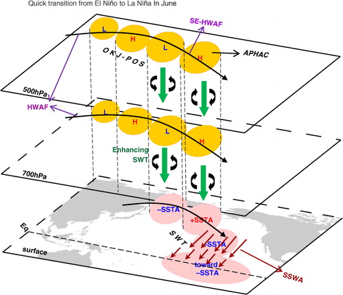
Fig. 10 The schematic of the quick transition from El Niño to La Niña: (1) The OKJ-POS dominates with barotropic structure in the middle and lower troposphere when El Niño has been decaying. The APHAC over about 30°N, 155°W with an anticyclonic rotation formed by propagation is shown. Upstream SE-HWAF further enhances all action-centres of the OKJ-POS teleconnection. (2) The SWT was generated in response to the propagation through the process of barotropic air–sea interaction, in which sea current has similar motion to the overlying flow. The SSWA forced out by the anticyclonic rotation on the east side of the APHAC can arrive into the EEP, which implies that the similar southward sea current could be generated in the southern SWT. This process plays a role in transporting cold water towards the EEP gradually. (3) The SWT can maintain itself for months without OKJ-like forcing or be enhanced by other types of SE-HWAF albeit with some phase shift southward. The transmission of the cold water from the SWT into the EEP keeps working and accelerates the decrease of the SST in the EEP with the reduction of the sea surface height in-situ so that La Niña matures completely in the following months.

7. Acknowledgements

We thank two anonymous reviewers for their valuable suggestions and comments. The first author thanks Ms. Yan Zhang for the assistant works for this paper. This study was supported by the project of the Ministry of Science and Technology of China (No. 2012CB417202), National Natural Science Foundation of China (No. 41375091) and the Special Fund of Laboratory of Severe Weather of China.

Notes

To access the supplementary material to this article, please see Supplementary files under Article Tools online.

1 They found a significant positive correlation between the Okhotsk high index during June and the SSTs in the Niño3 region in the preceding autumn. In fact, there is no significant correlation between the SSTs and the subsequent OKJ-JUN. However, the OKJ-POS statistically tends to accompany the development of the Okhotsk High that follows a previously strong El Niño event.

2 It is Pearson's cumulative test statistic, which was calculated by using the Minitab software. The alternate (null) hypothesis for cold events is that the occurrence of the cold events in Levels 1 and 3 of the OKJ-JUN is (not) mainly distributed in the Level 1. Similarly, the alternate (null) hypothesis for warm events is that the occurrence of the warm event is (not) mainly distributed in the Level 3.

3 Air masses generally flow out with clockwise rotation from anticyclone centre over Northern hemisphere. However, if the system has a large enough horizontal scale, the changes of the Coriolis force can cause the non-consistency in the rotation. Thus, the southerly flow on the west side of the anticyclone tends to move closer to the centre because of the Coriolis force getting larger with an increase in latitude. For the same reason, the northerly flow on the east side of the centre tends to move farther away from the centre. In the latter situation, a mass of fluid would escape from the anticyclone region and move farther southward. The SSWA on the southern end of the OKJ-POS even reached into the EEP (Figs 5a and 8a). Note that the real northerly wind speed is much larger than the anomaly in Figs 5 and 8.

References

- Battisti D. S . Dynamics and thermodynamics of a warming event in a coupled tropical atmosphere–ocean model. J. Atmos. Sci. 1988; 45: 2889–2919.
- Battisti D. S , Hirst A. C . Interannual variability in a tropical atmosphere–ocean model: Influence of the basic state, ocean geometry, and nonlinearity. J. Atmos. Sci. 1989; 46: 1687–1712.
- Bjerknes J . A possible response of the atmospheric Hadley circulation to equatorial anomalies of ocean temperature. Tellus. 1966; 18: 820–829.
- Bjerknes J . Atmospheric teleconnections from the equatorial Pacific. Mon. Wea. Rev. 1969; 97: 163–172.
- Chiang J. C. H , Vimont D. J . Analogous Pacific and Atlantic meridional modes of tropical atmosphere–ocean variability. J. Climate. 2004; 17: 4143–4158. http://dx.doi.org/10.1175/JCLI4953.1 .
- Deser C , Capotondi A , Saravanan R , Phillips S . Tropical Pacific and Atlantic climate variability in CCSM3. J. Climate. 2006; 19: 2451–2481.
- Giannini A , Kushnir Y , Cane M. A . Interannual variability of Caribbean Rainfall, ENSO, and the Atlantic Ocean. J. Climate. 2000; 13: 297–311.
- Hoskins B. J , Karoly D. J . The steady linear response of a spherical atmosphere to thermal and orographic forcing. J. Atmos. Sci. 1981; 38: 1179–1196.
- Kalnay E , Kanamitsu M , Kisler R , Collins W , Deaven D , co-authors . The NCEP/NCAR 40-year reanalysis project. Bull. Amer. Meteor. Soc. 1996; 77: 437–471.
- Kushnir Y , Robinson W. A , Bladé I , Hall N. M. J , Peng S , co-authors . Atmospheric GCM response to extratropical SST anomalies: synthesis and evaluation. J. Climate. 2002; 15: 2233–2256.
- Lupo A. R , Bosart L.F . An analysis of a relatively rare case of continental blocking. Quart. J. Roy. Meteor. Soc. 1999; 125: 107–138.
- Matthews A. J , Kiladis G. N . A model of Rossby waves linked to submonthly convection over the eastern tropical Pacific. J. Atmos. Sci. 2000; 57: 3785–3798.
- McPhaden M. J . Genesis and evolution of the 1997–98 El Niño. Science. 1999; 283: 950–954.
- McPhaden M. J , Zebiak S. E , Glantz M. H . ENSO as an integrating concept in Earth science. Science. 2006; 314: 1740–1745.
- Peixoto J. P , Oort A. H . Physics of Climate.
- Prabhu A , Mahajan P. N , Khaladkar R. M , Chipade M. D . Role of Antarctic circumpolar wave in modulating the extremes of Indian summer monsoon rainfall. Geophys. Res. Lett. 2010; 37: L14106. 5.
- Rasmusson E. M , Carpenter T. H . Variations in tropical sea surface temperature and surface wind fields associated with the Southern oscillation/ El Niño. Mon. Wea. Rev. 1982; 110: 354–384.
- Schopf P. S , Suarez M. J . Vacillations in a coupled ocean–atmosphere model. J. Atmos. Sci. 1988; 45: 549–566.
- Simmons A. J , Wallace J. M , Branstator G. W . Barotropic wave propagation and instability, and atmospheric teleconnection patterns. J. Atmos. Sci. 1983; 40: 1363–1392.
- Tziperman E , Stone L , Cane M. A , Jarosh H . El Niño Chaos: Overlapping of Resonances between the seasonal cycle and the Pacific Ocean–atmosphere oscillator. Science. 1994; 264: 72–74.
- Wallace J. M , Gutzler D. S . Teleconnections in the geopotential height field during the Northern Hemisphere winter. Mon. Wea. Rev. 1981; 109: 784–812.
- Wang Y . Effects of blocking anticyclones in Eurasia in the rainy season (Meiyu/Baiu season). J. Meteor. Soc. Japan. 1992; 70: 929–951.
- Wang Y , Lupo A. R . An extratropical air–sea interaction over the North Pacific in association with a preceding El Niño episode in early summer. Mon. Wea. Rev. 2009; 137: 3771–3785.
- Wang Y , Yamazaki K , Fujiyoshi Y . The interaction between two separate propagations of Rossby Waves. Mon. Wea. Rev. 2007; 135: 3521–3540.
- Wang Y , Yasunari T . A diagnostic analysis of the wave train propagating from high-latitudes to low-latitudes in early summer. J. Meteor. Soc. Japan. 1994; 72: 269–279.
- Wang Y , Zhai P , Qin J . Construction of the OKJ teleconnection index. Theor. Appl. Climatol. 2013; 111: 303–314.
- Wytrki K . The dynamic response of the equatorial Pacific Ocean to atmospheric forcing. J. Phys. Oceanogr. 1975; 5: 572–584.
- Zhang L , Chang P , Ji L . Linking the Pacific Meridional Mode to ENSO: Coupled Model Analysis. J. Climate. 2009; 22: 3488–3505. http://dx.doi.org/10.1175/2008JCLI2473.1 .