Generation and transfer of internal variability in a regional climate model

Abstract

There is a strong need for tools allowing the comparison between the performance of a regional climate model (RCM) and the corresponding model providing lateral boundary conditions (LBC) for the RCM, which is a global general circulation model (GCM) in most cases. A method is presented to investigate the temporal scales on which a RCM is able to generate internal variability on its own and on which variability is copied from the driving model. This is implemented by a cross-spectral analysis between the RCM output and a bi-linearly interpolated version of the driving model, leading to an estimate of the coherence spectrum. Applying the aforementioned technique to surface temperature and temperature and specific humidity at 850 hPa from the RCM COSMO-CLM East Asia with a horizontal resolution of 50 km and its driving model ECHAM5, it was found that features in the spatial distribution of coherence are related to atmospheric dynamics in East Asia, e.g. monsoons and inter-tropical convergence zone (ITCZ). A further application to a double-nesting approach, where COSMO-CLM East Asia is the driving model for two domains – namely the Haihe catchment and the Poyang catchment – each with a horizontal resolution of 7 km, shows that the frequencies on which internal variability is generated by the driven model are much higher compared to the first nesting step. Concluding RCMs can produce a considerable variability on the respective temporal scales. This implies that a dynamical downscaling with a re-analysis as LBC is conceptually different to a regional re-analysis, i.e. data assimilation on the regional scale.

• East Asia
• COSMO
• cross-spectrum
• internal variability
• dynamical downscaling
• nesting
• double-nesting

1. Introduction

Assessing and projecting climate change is usually based on global general circulation models (GCMs). Due to high computational cost, the spatial resolution of GCMs is limited. This results in grid boxes with areas of the order of 10⁴ km ² (Roeckner et al., 2003; Uppala et al., 2005) and even lower effective resolutions. Studies investigating the energy spectra of numerical weather prediction models (NWPs) (Skamarock, 2004; Bierdel et al., 2012) suggest effective resolutions about 4–7 times coarser than the original grid. In addition, the low horizontal resolution of GCMs leads to a weak representation of local extreme events (Easterling et al., 2000), which is associated with the change of support effect (Wackernagel, 2010).

To add additional regional information to the global input and to keep computational cost on an acceptable level, dynamical downscaling via regional climate models (RCMs) (e.g. Giorgi et al., 2001; Frei et al., 2006; Gao et al., 2008; Rummukainen, 2009) became an established method over the past 10–20 yr. The popularity of RCMs is also caused by the increasing demand for high-resolution data from other disciplines, e.g. hydrology, biology (e.g. Kuemmerlen et al., 2012; Schmalz et al., 2012). This led the World Climate Research Programme (WCRP) to establish the Coordinated Regional Climate Downscaling Experiment (CORDEX) with the goal to coordinate and to keep record of RCM simulations undertaken by research groups all over the world (Giorgi et al., 2009). Within CORDEX, 13 RCM domains are defined covering the globe. Examples of a CORDEX-based effort are the RCM ensemble simulations performed for Europe (EURO-CORDEX, see Vautard et al., 2013), Africa (CORDEX-Africa, see Nikulin et al., 2012) and within the North American Regional Climate Change Assessment Program (NARCCAP, see Mearns et al., 2012).

One conceptual shortcoming of RCMs is emphasized here, as it is closely related to the generation of internal variability in RCMs. While GCMs integrate the coupling between multiple components of the climate system – at least atmosphere and ocean (hydrosphere), but also cryosphere, biosphere and lithosphere – RCMs restrict the coupling usually to biosphere and lithosphere via so-called land surface models (Giorgi et al., 2001). Due to the usually applied one-way nesting technique of RCMs – as it is also the case in our simulations – one drawback of these simulations is that teleconnections are not included and hence large-scale climate feedbacks are suppressed. For example, in a RCM adapted to East Asia the monsoon systems do not influence ENSO, while ENSO signals are transmitted via lateral boundary conditions (LBC) as it was simulated in the driving GCM (Wang et al., 2005). Furthermore, air–sea interactions are no part of most RCM simulations as the SST of the driving GCM is often used as a lower boundary instead of a dynamical ocean component (Hagedorn et al., 2000) or at least a slab ocean, which would model the damping effect of the ocean mixed layer and hence allow to store heat in the ocean (Lorbacher et al., 2006; Dommenget, 2010).

The main purpose of RCM simulations is to explicitly resolve and thus not to parameterize processes at finer spatial and temporal scale. Therefore, internal variability is generated on scales, which are not modelled by global GCMs. This self-generated internal variability is often referred to as added value of a RCM simulation compared to a GCM, though added value is often also defined as the ability of a RCM to modify the externally forced variability. After all, there is still demand for basic research about the credibility of RCMs. Therefore, there is a strong need for studies on the comparison of RCM simulations and their driving models (Laprise et al., 2008; Feser et al., 2011). After reviewing literature (see references below), three categories of different definitions of added value can be identified. In the first category, added value is defined in terms of estimating the level of the change of support effect between global and regional simulations compared to point-like observations. In the second and third category, added value is described as the gain of internal variability at small spatial and temporal scales, respectively.

The definition of added value on the basis of verification has been applied in studies dealing with different models, e.g. regional models driven by re-analysis data, NWP models and regional models driven by global climate simulations. Feser (2006) compared two RCM simulations – with and without spectral nudging (von Storch et al., 2000) – and the NCEP re-analysis with the analysis generated by the model run operationally at Germany's National Meteorological Service (DWD). Applying a spatial filter technique to separate spatially large and regional scale signal, it was found that the spectrally nudged RCM leads to the best reproduction of the observations. The investigation of a double-nesting approach for East Asia showed the ability to reconstruct single events like typhoons more realistically than in the original re-analysis data (Feser and von Storch, 2008). A comparison between near surface wind speed of spectrally nudged RCM simulations driven by re-analysis data and QuikSCAT observations exhibited added value, especially along coastlines and for regions with complex terrain (Winterfeldt and Weisse, 2009). Using a verification approach based on Bayesian statistics, Röpnack et al. (2013) showed the ability of the COSMO-DE convection permitting ensemble prediction system (COSMO-DE-EPS, 2.8 km grid) to forecast the probability of tropospheric temperature profiles in a superior manner compared to two other COSMO-based ensembles (each 10 km grid). Another study falling in this first category is an analysis of the NARCCAP ensemble (Di Luca et al., 2012). This analysis does not use the original data of the driving model, but uses an upscaling technique for the RCM output, which works as a filter for high-resolution variability. The added value of a RCM is defined as the improvement of the representation of climate statistics, e.g. the 95th quantile of precipitation. Thus, this first category is not restricted to studies dealing with re-analysis and NWP models, and also includes studies investigating climate simulations.

There are different approaches to assess added value in terms of spatial small-scale variability, which refers to the second category of definitions. Via spatial spectral analysis (Errico, 1985) of kinetic energy and moisture flux convergence, it was revealed that the RCM increases variability on smaller scales in comparison to the driving re-analysis (Rockel et al., 2008a). Using the same spectral technique, it was found that the sensitivity of a RCM to surface forcing depends on the implemented convection scheme (Castro et al., 2005). A special way to evaluate the added value of a RCM is the so-called ‘Big-Brother Experiment’ (BBE) (Denis et al., 2002). Here, both a Big-Brother and a Little-Brother have to be generated by a RCM and compared afterwards, with the Big-Brother working as a mentor for the Little-Brother: First, the high-resolution Big-Brother data is filtered to remove fine-scale variability. Second, the filtered Big-Brother is used as a driving dataset for the Little-Brother. This allows us to evaluate RCM specific errors. The downside of this method is the high computational costs. Nevertheless, an important outcome of studies analysing BBEs is that the merit of a RCM simulation emerges rather when a large domain is setup than in the case of a smaller domain. In the first case, more internal variability on small spatial scales develops compared to the second case (Laprise et al., 2012).

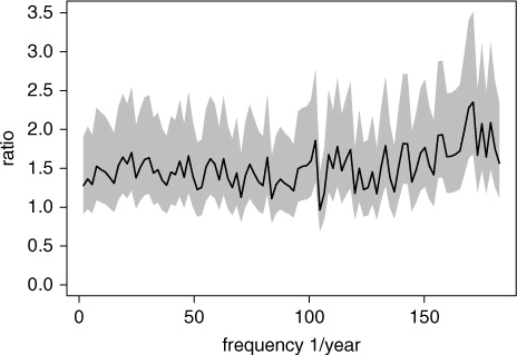
We follow a third way of defining added value. Added value is the ability of the regional model to generate internal variability on temporal frequencies in opposition to variability that is transferred from the driving model. The ratio of the univariate spectra of both models – computed with time series of single grid boxes that have close to equal locations – shows the increase of variance in the RCM (Fig. 1). However, we are aiming at investigating the contribution of the RCM in terms of developing dynamics on small temporal scales. This kind of approach is feasible with coherence spectra between both models (Section 3).

Fig. 1 Exemplary ratio of the RCM spectrum and the GCM spectrum for one grid cell in the Pacific (140°E, 20°N) for T850 in winter taken from the ‘20C’ experiment. The shaded area indicates the 95% confidence interval.

Considering the effective resolution of a circulation model, which is known from experimental studies on the mesoscale to be about 4–7 times coarser than the original grid (e.g. Bierdel et al., 2012), leads to a rough estimate for the spatial scales. The 50-km horizontal grid spacing of a RCM runs would result in an effective resolution of 200–350 km. The driving model ECHAM5 has a horizontal resolution of T63, which equals a resolution of 630 km at the equator in spectral space. Added value would then be expected at spatial scales from 350 to 600 km. The corresponding temporal scales with respect to atmospheric processes lie in a range between 1 h and 1 d (Orlanski, 1975), but this rough estimate for the temporal scales leaves open the question as to whether the involved regional model has the ability to develop dynamics on these scales.

In this paper, we address the problem, on which temporal scales added value can be expected. A method, based on cross-spectral analysis (Section 3), is proposed to investigate the potential of a RCM to adapt and self-generate internal variability. The method is applied to simulations over East Asia with COSMO-CLM and ECHAM5. Both a nesting and a double-nesting approach are analysed (Section 2). The results presented in detail in Section 4 are discussed in Section 5, with the focus set on special issues that require further explanations and on added value of RCM simulations in general. Special attention is given to a conceptual formulation of the methodology (Section 6). Section 7 contains concluding remarks and proposes further applications for the method.

2. Data

The basis for this study is RCM simulations for East Asia (Fig. 2) performed with the COSMO-CLM (COnsortium for Small-scale MOdelling–Climate Limited area Model, Rockel et al., 2008b). The domain covers both tropical and extra-tropical regions. The centre of the domain is located above eastern China, where the East Asian Summer Monsoon dominates the regional climate during summer (Ding and Chan, 2005; Simon et al., 2013). The model is integrated on a 0,44°grid (about 50 km) and forced by LBC once every six hours, using a sponge zone with a width of 10 grid points on each side. One run is forced by ECHAM5 20C3M_all run no.3 (hereafter: ECHAM5) (Roeckner, 2005), another one by ECHAM5 A1B run no.3, and a third run by the ECMWF 40 yr Re-analysis (ERA-40) (Uppala et al., 2005). For further details on the adaption of COSMO-CLM to the domain and on physical and numerical parameters, the reader is referred to Wang et al. (2013). However, an extract of the model parameters is given in Table 1. Wang et al. (2013) also discussed how typical summer and winter weather phenomena for East China are represented in the model. The basic concept of the analysis is the comparison of the output of the driving model with the output of the driven model. To this end, the coarse data (ECHAM5, ERA 40) is bi-linearly interpolated to the grid of COSMO-CLM. For the spectral analysis (cf. Section 3), only daily mean values were used. The main focus is set on temperature at 2 m (T_2M), temperature at 850 hPa (T850) and specific humidity at 850 hPa (Q850). This choice of variables allows us to analyse differences of the properties at the surface and in the lower atmosphere (T_2M vs. T850), as well as to account for specific features for the water cycle (Q850 vs. T850).

Fig. 2 Orography [m a.m.s.l.] for the East Asia domain in 0,44°resolution. The grey frame indicates the sponge zone. Two subdomains (North—Haihe, South—Poyang) are highlighted by boxes.

Table 1. Simulations performed with COSMO-CLM for East Asia

Single-nesting	Double-nesting Haihe	Double-nesting Poyang
Model	COSMO_4.8_CLM_11 (and higher)
Horizontal resolution	0,44° (50 km)	0,0625° (7 km)
Horizontal grid size (excl. sponge zone)	183×147	160×160	128×144
Timestep	150s	60s
Convection scheme	Tiedtke
Time interval for boundary conditions	6 hours
Driving model & simulated period	ERA40 1971–2000 (CCLM_eval_50km)	CCLM_eval_50km 1971–2000	CCLM_eval_50km 1971–1975
ECHAM5_20C3M_all_3 1971–2000 (CCLM_20C_50km)	CCLM_20C_50km 1971–2000	CCLM_20C_50km 1971–1997
ECHAM5_A1B_3 2011–2050 (CCLM_A1B_50km)	CCLM_A1B_50km 2021–2050	CCLM_A1B_50km 2021–2050

In addition to the 0,44° model, a double-nesting approach has been applied to two smaller regions simultaneously. The motivation for the double-nesting approach is to enter a very fine spatial resolution representing more details of the topography. The first region is the catchment of the Haihe river in the Northeast of China, and the second region is the catchment of the Poyang lake in the Southeast of China (Fig. 2). The resolution for both of these domains is 0,0625° (7 km), but the areal extend of both domains differs. The calculation was run on a 160×160 and a 128×144 grid (excluding the lateral sponge zone) for the Haihe catchment and the Poyang catchment, respectively. These simulations were driven by the output of the 50 km run forced by ECHAM5 20C3M. Again, the output of the 50 km run is bi-linearly interpolated to the grids of the Haihe domain and the Poyang domain, respectively. As the spatial resolution of the model is finer – 7 km vs. 50 km – added value is also expected on shorter time scales. Therefore, the data was taken in a temporal resolution of one value per hour for this analysis, which is only available for T_2M. An overview of the simulations performed for East Asia by COSMO-CLM and an extract of the model parameters is given in Table 1.

3. Methods

The basis of our methodology is a cross-spectral analysis. Before the estimation of the spectral parameters can be applied, the time series should be filtered from obvious periodic signals, e.g. (semi-) annual cycle and diurnal cycle, which is done by a standard linear regression model fitted to the time series at each grid point. For the comparison between the COSMO-CLM 50 km run and its driving model, ECHAM5, the purpose of the linear regression is to detect the annual and semi-annual cycle, as both extra-tropics and tropics are included in the East Asia domain. The diurnal cycle is excluded from the time series, as the data for this comparison is daily mean values.1

The indices m, lt, ac and sac stand for mean, linear trend, annual cycle and semi-annual cycle, respectively. X′ represents the filtered time series, which will be analysed later. Both annual cycle and semi-annual cycle are described by two parameters: amplitude and phase shift of a sine signal at the annual and semi-annual frequencies. For most regions, σ ² depends on the season, thus X′ will be analysed conditioned on the season. In this analysis (ECHAM5 vs. COSMO-CLM 50 km), we consider the summer season, from April to September, and the winter season, from October to March, which results in about 180 data values per season and year.

For the comparison between the COSMO-CLM 7 km runs and its driving model, COSMO-CLM 50 km, hourly values are available. First, the summer season, from June to August (JJA), and the winter season, from December to February (DJF), were selected from the time series. The selected seasons differ in length compared to the seasons selected above due to computational aspects. Hourly values and seasons of three months in length result in about 2160 values per season and year. Second, to detect the diurnal cycle, a linear regression model has been fitted to each season individually:2

Here, the diurnal cycle term X_dc consists of 24 parameters, one for each hour of the day. In Section 4, we will see that the relevant time scale, on which the driven RCM changes from transfer to generation of variability, is about 1 d. In order to avoid aliasing effects (Von Storch and Zwiers, 2002) from sampling high frequency signals at low rates, only temperatures at 2 m, which are available with hourly resolution, will be analysed for the step from 50 to 7 km resolution.

To examine this nature of co-variability between the driving model and the driven model over a continuum of frequencies, the cross-spectra3

are estimated grid-point wise. Here, denotes the Fourier transform, γ _xy stands for the cross-covariance function of the time series X and Y. On the right-hand side of eq. (3), the cross-spectrum is expressed in polar coordinates, where A_xy and Φ _xy are called amplitude spectrum and phase spectrum, respectively. However, the amplitude of the complex cross-spectrum Γ _xy will be represented as squared coherency spectrum,4

Γ _xx and Γ _yy refer to the univariate spectra of the time series X and Y, respectively. The coherence is dimensionless and formally similar to the squared correlation. Thus, the coherence function can be seen as a linear transfer function of information from the driving model to the driven model (Jenkins and Watts, 1968). Due to the experiment setup, a phase lag of a climate signal occurring in both models is unexpected and the phase spectrum can be neglected.

Technically, the estimation of the cross-spectrum is based on bi-variate periodograms. As the pure bi-variate periodogram is not a good estimator for the cross-spectrum, smoothing techniques have to be applied (Jenkins and Watts, 1968; Von Storch and Zwiers, 2002). For the frequency 1/yr, a Daniell spectral estimator was used. For higher frequencies, the time series was split into blocks of the same length called chunks. The periodograms computed individually for each chunk are averaged afterwards in order to account for different variances σ ² of the residual time series conditioned on the season. To keep the inference of both the Daniell spectral estimator and the chunk spectral estimator consistent, it was ensured that both estimators result in about the same degrees of freedom. Uncertainty of the estimation is assessed via 95% confidence intervals. For more details on the applied estimators, the reader is referred to Von Storch and Zwiers (2002).

4. Results

The results for the first nesting step, i.e. from ECHAM5 to COSMO-CLM 50 km, are presented first, followed by the comparison of COSMO-CLM 50 km and the double-nesting COSMO-CLM 7 km for the two catchments, Haihe and Poyang.

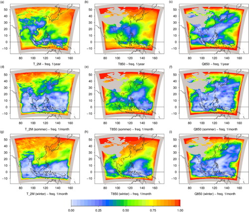
Appearing for all examined variables and frequencies is a red frame along the lateral boundaries (Fig. 3), where coherence is close to unity. This indicates a strong transfer of climate variability at the boundaries, which can be expected due to the experimental setup. The width of the red frame varies between the different variables, but is of the order of the width of the sponge zone, which is 10 grid boxes at each side in our setup.

Fig. 3 Grid-point wise coherence between COSMO-CLM (0,44°resolution) driven by ECHAM5 20C3M_all run no.3 and ECHAM5 20C3M_all run no.3. The 1st, 2nd and 3rd columns show results for the variables T_2M, T850 and Q850, respectively. The 1st, 2nd and 3rd rows show results for the frequencies 1/yr, 1/month in summer and 1/month in winter, respectively. The grey frame indicates the sponge zone. The grey shaded areas within the domain cover mountainous regions, that lie above 850 hPa.

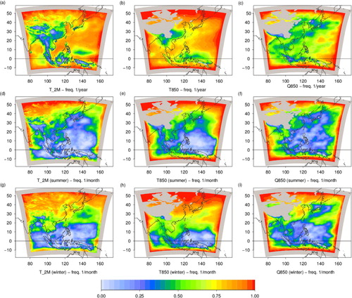
For the variables T_2M, T850 and Q850, more variability in the spatial patterns of coherence at frequency 1/yr is found in the inner domain (Fig. 3a–c). The field for T_2M exhibits a pronounced land–sea contrast, with a strong transfer of variability over the ocean and a weak transfer over land (Fig. 3a). This is especially apparent for the tropics with its large islands and the Indochinese peninsula, but it is also visible in the extra-tropics at the coastlines of East China, Korea and southern Japan. Here, one should keep in mind that the sea surface temperature of ECHAM5 serves as a boundary condition and drives COSMO-CLM from the ocean. Exceptions to this general image are found in the higher latitudes of the domain, where for both land and sea a strong transfer of variability can be detected, and over the tropical ocean at 5°N to 10°N in the eastern part of the domain, where a local minimum of coherence is located (cf. Section 5).

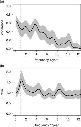
To investigate the coherence spectrum at this local minimum over a range of frequencies, we averaged the 2 m temperature, over the box 4°N to 9°N and 132°E to 144°E, before calculating the spectrum (Fig. 4a). This procedure also cancels out fine-scale variability. The coherence is about 0.5 at 1/yr and decreases close to zero at 1/month. This result matches with the values presented in the maps. For completeness, the ratio between the univariate spectra of the two models is also computed (Fig. 4b). The ratio gives a measure of the absolute similarity. Though the variability of T_2M in COSMO-CLM is higher than in ECHAM5 at the frequency 1/yr, it is still in the same order.

Fig. 4 Analysis of T_2M averaged over the box 4°N to 9°N and 132°E to 144°E. (a) Coherence between the time series from COSMO-CLM driven by ECHAM5 20C3M_all run no.3 and ECHAM5 20C3M_all run no.3. (b) The ratio between the corresponding univariate spectra.

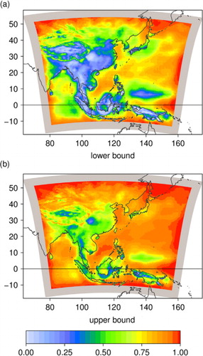
To give an impression of the uncertainties coming along with the estimator, a closer look is taken at the 95% confidence interval for T_2M at the frequency 1/yr (Fig. 5). The most important feature is the local minimum around 10°N in the Pacific, which remains even in the upper bound of the confidence interval. In the lower bound, the degree of decoupling is pronounced over East South Asia and the area South of the equator in the Indic exhibits a local minimum with values around 0.5.

Fig. 5 95% confidence interval for T_2M at the frequency 1/yr (Fig. 3a).

In the lower troposphere at 850 hPa, the temperature reveals a slightly different image (Fig. 3b). For most of the domain, a strong transfer of variability is obviously similar to T_2M, but the pronounced land–sea contrast over the tropics has weakened towards higher coherence values over the land. A possible explanation is the stronger dependence of T_2M on the parameterisation of land surface processes, which differs between ECHAM5 and COSMO-CLM and hence leads to low coherence between the models at 2 m. Another difference between the spatial pattern of T850 and T_2M is a shift of the local minimum over the tropical North Pacific further South closer to the equator. Both minima are connected vertically, which was checked with a cross-section at 135°E (figure not shown). Furthermore, compared to the pattern of T_2M, the transfer of variability over the Asian landmass is more enhanced. Only very close to the mountain range, where the temperature at 2 m coincides with the temperature at 850 hPa, low coherence values are found.

While variability of temperature at 850 hPa is strongly dictated by ECHAM5, the variability of specific humidity at 850 hPa is rather decoupled (Fig. 3c). Even the green areas (κ _xy (1/year) = 0.5) indicate that still 50% of the variance in the RCM can be explained by the driving GCM. However, this finding suggests a decoupling of the modelled water cycle.

In general, the results for the frequency 1/month (Fig. 3d–i) exhibit that the RCM is decoupled from its driving model in the inner domain with coherence values <0.25 for large areas of the domain. The extent of this ‘inner domain’ varies for the different variables and seasons. For summer (Fig. 3d–f), the areas, for which the driven and the driving model are decoupled from each other, reach further North than in winter (Fig. 3g–i); the Asian landmass is covered with coherence values >0.5 in winter, with the lower coherence for Q850 over the Indochinese peninsula being the only exception. Over the Bay of Bengal, both variables (temperature and humidity) at 850 hPa are influenced by the driving model stronger in summer (Fig. 3e,f) than in winter (Fig. 3h,i), which can be associated with the prevailing southwesterly trade winds in this region.

Similar to the results for the frequency 1/yr, there is a stronger coupling between ECHAM5 and COSMO-CLM for a temperature at 850 hPa than for humidity at the 1/month frequency. For Q850, coherence values less than 0.5 extend even to the northeastern part of the domain. In contrast, the decoupling for T850 is more concentrated on tropical regions, which is especially true for the winter (Fig. 3h).

Comparing T_2M and T850 exhibits similar patterns for the coherence values at the frequency 1/month. However, the influence of ECHAM5 on the temperature in COSMO-CLM is slightly stronger at 850 hPa than at the surface. This is remarkable, as the ECHAM5 SST serves as a boundary condition for the RCM runs. Parameterized processes at the surface might cause the strong decoupling between the surface temperatures in the models.

For the sake of completeness, the results of the cross-spectral analysis between COSMO-CLM driven by ECHAM5 under the A1B scenario reveal nearly the same spatial coherence pattern as under the 20C conditions (Fig. 3). All correlations between the 20C coherence pattern and the corresponding A1B pattern exceed 0.9. This circumstance should only be mentioned here as it makes the results for 20C more robust, but a presentation of the results for A1B in detail can be omitted.

Figure 6 shows an extract of the results gained from the comparison of the two 7-km domains (namely Haihe catchment and Poyang catchment) with their driving counterpart at the 1/48 h frequency. As discussed in the Methods section, only a temperature at 2 m is analysed. Similar to the first nesting step, coherence values for summer (JJA) are smaller than for winter (DJF). This finding indicates that convective-scale processes typical for summer are generated in the driven model independent from the processes passed by the 50-km driving model, which leads to a decoupling in the surface temperature. The reason for the decoupling might be found in the different applicability of the Tiedtke convection scheme on the different resolutions (Kuell et al., 2007). In contrast, the large-scale processes typical for winter lead to the transfer of variability in the surface temperature.

Fig. 6 Grid-point wise coherence at frequency 1/48h between COSMO-CLM (0,0625°resolution) driven by COSMO-CLM ‘20C’ (0,44°resolution) and COSMO-CLM ‘20C’ (0,44°resolution). The 1st and 2nd columns show the results for COSMO-CLM (0,0625°) adapted to the Haihe catchment and the Poyang catchment, respectively. The 1st and 2nd rows show the results for summer season (JJA) and winter season (DJF), respectively. The grey frame indicates the sponge zone.

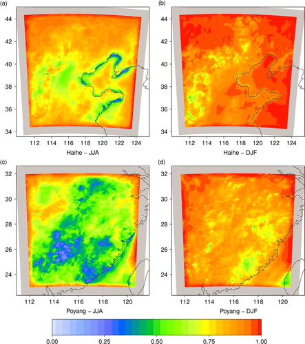
Comparing the coherence distribution in both domains with each other, we find smaller values for the Poyang catchment. We suppose that day-to-day variability in the Poyang basin is dominated strongly by monsoon dynamics, which is associated with higher variability in small-scale features, compared to the weather in the Haihe region (Wang, 2006; Simon et al., 2013). Although a similar dipole structure is already visible in the results of the first nesting step (Fig. 3d), the results in Fig. 3 cannot be directly compared with the results in Fig. 6. These findings are absolutely independent from each other, as no ECHAM5 information is integrated in the analysis of the second nesting steps. Another remarkable feature is the band of relatively low coherence values along the coastline in the Haihe domain for the JJA season (Fig. 6a), which is a direct effect of the change from low to high resolution and the attended better representation of the land–sea mask. In winter (DJF), where coherence is high for the whole domain, the minima lie in the mountainous regions. This is an effect of orography, which is represented more realistically in COSMO-CLM at higher resolution.

However, the fact that for the Poyang catchment coherence values less than 0.5 m at the frequency 1/48h were found for large parts of the domain is a sufficient condition for an expected added value of further analyses, such as the application of extreme value theory on weather extremes associated with a daily time scale (Katz et al., 2002; Friederichs, 2010). The strong transfer of variability for the winter months indicates that there is no potential to expect added value in terms of additional variability on high temporal frequencies. For completeness, it is tested for added value in terms of modification of the amplitude of the input signal. This is done via the ratio of the univariate spectra of both models (not shown). For our example, this aspect of added value could be detected at some isolated spots. Furthermore, our methods provide no sufficient condition to reject the potential of the RCM to generate more variability on high spatial frequencies, which can be assessed by the method presented by Errico (1985).

5. Discussion

In this section, two key aspects will be addressed. On the one hand, we suggest an explanation for the local minimum of coherence in the T_2M field for the frequency 1/yr over the tropical North Pacific. On the other hand, we discuss transfer and generation of climate variability in RCMs in general.

In order to investigate the local minimum in Fig. 3a, we take a closer look at the precipitation distribution generated by COSMO-CLM and ECHAM5, which is closely related to the dynamics of the inter-tropical convergence zone (ITCZ) (Fig. 7). In this region, with its dominant easterly trade winds, ECHAM5 directly feeds COSMO-CLM. A typical feature of ECHAM5 in the tropical Pacific is the so-called double ITCZ, which is a well-known phenomenon in most coupled GCMs (Li et al., 2004). This leads to a northern ITCZ, broadened and shifted further North compared to observations that persist throughout the year (Jungclaus et al., 2006). In the precipitation field of ECHAM5 (Fig. 7b), the northern ITCZ is clearly visible as a strong rain belt around 10°N in the Pacific.

Fig. 7 Comparison of mean annual precipitation from COSMO-CLM and ECHAM5 for the period from 1971 to 2000 in mm. The field of ECHAM5 is bi-linearly interpolated to the COSMO-CLM grid and the sponge frame is added for better visual orientation. The right-hand plot shows the relative change between COSMO-CLM values and ECHAM5 values, with the darkest red indicating a relative change of –100% or less.

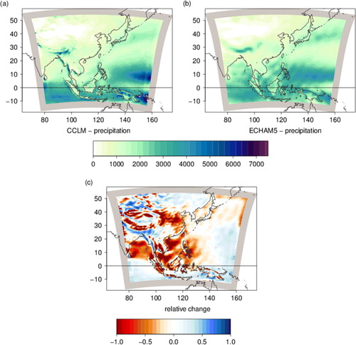
When this strong precipitation belt enters the RCM domain, it has to get adapted to the new grid. The ECHAM5 ITCZ transports a huge amount of moisture into the COSMO-CLM domain. The major part of this humid air accumulates close to the boundary, where mean annual precipitation up to 7000 mm/year is simulated. This is a strong positive wet bias compared to the mean annual precipitation in ECHAM5. About 95% of the simulated precipitation in COSMO-CLM in this region is related to convective processes, which depend on the applied parameterisations. Following the ITCZ in COSMO-CLM to the East the mean annual precipitation values decrease. The sign of the bias changes at about 140°E and close to the Philippines the bias reaches strong negative values. This finding indicates a strong dissonance between the convection schemes of the two models. In turn, this could cause the decoupling (κ _xy (1/year)~0.5) of the variability of the 2 m temperature in COSMO-CLM and the variability of 2 m temperature in ECHAM5. Further parameter tuning, e.g. adjustment of the Rayleigh sponge damping layer (Wang et al., 2013), could help to reduce this dissonance.

We now enter the discussion about transfer and generation of climate variability in RCMs in general. To this end, we review the results of a second experimental setup and examine the coherence spectra between COSMO-CLM driven by ERA-40 and ERA-40 itself (Fig. 8). The applied LBC differ from the ones of the ECHAM5 driven experiment, which helps to gain information about the influence of the LBC versus the potential of the RCM to develop an independent inner domain. The spatial resolution of ERA-40 is higher than the spatial resolution of ECHAM5, which leads potentially to more fine-scale variability that is directly passed into the regional model.

Fig. 8 Grid-point wise coherence between COSMO-CLM (0,44 °resolution) driven by ERA-40 and ERA-40. The 1st, 2nd and 3rd columns show results for the variables T_2M, T850 and Q850, respectively. The 1st, 2nd and 3rd rows show results for the frequencies 1/yr, 1/month in summer and 1/month in winter, respectively. The grey frame indicates the sponge zone. The grey shaded areas within the domain cover the mountainous regions that lie above 850 hPa and contain only artificial results for T850 and Q850.

The results based on ERA-40 (Fig. 8) are similar to the ones based on ECHAM5 (Fig. 3) with respect to the high coherence values near the boundaries and on the landmass in the North and low values in the inner domain, particularly in the tropics. Strong similarities prevail for the frequency 1/month, which leads to the conclusion that the patterns for transfer and generation of variability on this frequency are mainly based on the model itself, COSMO-CLM. Stronger differences can be seen at the frequency 1/yr with a distinct feature related to the ITCZ in the eastern part of the tropics (Fig. 8a). In contrast to ECHAM5, there is no persistent double ITCZ in ERA-40 and accordingly the associated LBC differ strongly from each other. Another remarkable feature is the decoupling of the water cycle (i.e. Q850, Fig. 8c) between COSMO-CLM driven by ERA-40 and ERA-40, which is even more pronounced compared to the ECHAM5 case (Fig. 3). There are different possible explanations for this finding. On the one hand, this finding might be related to the fact that intrinsic model noise is abandoned in ERA-40 and replaced by observational noise. On the other hand, one could also expect such a difference if the physical parameterisations (e.g. boundary layer, shallow convection, etc.) that affect Q850 differ more between ERA40 and COSMO-CLM than between ECHAM5 and COSMO-CLM.

The experiment with LBC from ERA-40 reveals that a dynamical downscaling driven by re-analysis data is conceptually different to a regional re-analysis, which would include data assimilation on the regional scale. The results (Fig. 8) show that COSMO-CLM generated variability in the inner domain by itself. Within a regional re-analysis framework, this freely developing variability would be suppressed by the data assimilation.

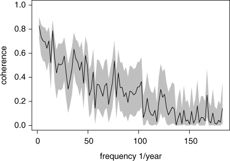
Finally, although the significance of the presence of self-generated climate variability cannot be assessed quantitatively due to the lack of appropriate test statistics (cf. Section 3), a qualitative statement can be made. Looking at an example of a coherence spectrum for one grid cell (Fig. 9), it is obvious that a decay of coherence takes place over a broad band of frequencies rather than a sharp drop.

Fig. 9 A exemplary coherence spectrum for one grid cell in the Pacific (140°E, 20°N) for T850 in winter taken from the ‘20C’ experiment. The grey shaded area indicates the 95% confidence interval.

6. Conceptual model

In this section, we are formulating an approach to assess the analysed aspect of added value theoretically.

The purpose of this method is to find the frequency band on which the RCM simulations copy the internal variability of the driving model and on which the RCM potentially generates internal variability on its own. The first and the latter frequency bands refer to slow and fast variations in the time series, respectively. Conceptually, one can imagine a decomposition as follows:5 6

with the following indices: the driving model (driving), slow varying variability (sv), noise (n), the driven model (driven), adapted variability (av), self-generated variability (sgv). This conceptual model allows us to interpret the co-variability between X _driving and Y _driven,7

as a function of the time scale. A high correlation can only be expected between X _gv and Y _av All terms, in which noise is taken into account, the correlation equals zero by definition. One should keep in mind that X _gv and Y _av are not necessarily truncated at the same frequency, but there might also be a band of frequencies, which is populated by both X _gv and Y _sgv Therefore, the correlation between X _gv and Y _sgv is not necessarily zero, but rather is expected to show a decay for the correlation towards shorter time scales.

Within this framework, it can be considered how a proper hypothesis testing for the above analysis could be designed. Usually a coherence value has to be tested against H ₀:κ _xy=0. Considering our conceptual model [eqs. (5) and (6)], this type of test is not appropriate for our problem. The question to be answered would be whether the self-generated internal variability of the driven model is greater than zero H ₁:E(Y′ _sgv ²) > 0. Formally, this means to test H ₀:E(Y′_sgv ²) = 0, which cannot be easily assessed.

7. Conclusions

This study introduces a method defining one aspect of added value in terms of ability of the regional model to generate variability on its own. With this technique, it is possible to analyse the temporal scales on which internal variability is generated by the RCM itself and on which variability is dictated by the driving model (a GCM in most cases). This method does not account for added value in term of a modification of the amplitude of the input signal, which can be tested by the ratio of the univariate spectra of the two models. Though not applied in this study, coherence spectra might also be used in studies dealing with added value on spatial scales.

An example – COSMO-CLM East Asia – illustrates the problems that can be assessed with this method. Self-generated variability was found in the 50-km RCM already on temporal frequencies between 1/yr and 1/month. In a second nesting step, i.e. from 50 to 7 km, variability in the driven model was dictated by the driving model even up to a day-to-day scale. That is a vast difference of temporal scales between the two nesting steps. The method was also applied to COSMO-CLM driven by the re-analysis ERA-40. The circumstances that the method reveals self-generated variability in the RCM output make clear that this simulation is conceptually different to a regional re-analysis, in which a data assimilation scheme is implemented (e.g. Mesinger et al., 2006).

A straightforward benefit of this method is that it gives insights in the usability of RCM output for further studies, e.g. the representation of extreme events (e.g. Katz et al., 2002; Friederichs, 2010), statistical downscaling (e.g. Benestad, 2004; Simon et al., 2013). Questions concerning the influence of numerical parameters on RCM performance arising from this study include:

• the sensitivity of the temporal scale between adapted and self-generated climate variability to the choice of domain size

• the role of the chosen RCM, i.e. is there a certain setup supporting the ability of the RCM to generate variability by its own

• the effect of differences in the LBC, which inserts systematic errors from the driving model

• the influence of a dynamical ocean component or a conceptual model like a slab ocean compared to a prescribed SST.

All of these questions are beyond the scope of this study, but can probably be assessed by applying the method or an extension of the method on multi-RCM ensembles, which are available, e.g. for Europe (EURO-CORDEX, see Vautard et al., 2013) and Africa (CORDEX-Africa, see Nikulin et al., 2012) and North America (NARCCAP, see Mearns et al., 2012).

8. Acknowledgements

The authors gratefully acknowledge two anonymous reviewers for their comments. This work was funded by the NSFC/DFG-joint funding programme Land Use and Water Resources Management under Changing Environmental Conditions. It was also carried out in the Hans Ertel Centre for Weather Research, a research network of Universities, Research Institutes and the Deutscher Wetterdienst funded by the BMVBS (Federal Ministry of Transport, Building and Urban Development). Furthermore, the authors would like to thank Christoph Menz from BMBF's Guanting Project for the smooth and straightforward supply of data. The authors would like to credit the contributors to the R project.

Notes

¹In geostatistics support is the interval, surface or volume, for which a value represents the average. The change of support effect refers to the circumstance that the variance of a variable averaged over an extended area, e.g. a grid-box, has to be less than the variance at a local point. (Wackernagel, 2010).

²The ECHAM5 20C3M_all simulations are driven with anthropogenic forcing (CO₂, CH₄, N₂O, CFCs, O₃ and sulphate) and natural forcing (variable solar forcing and effect of volcanic aerosols).

³The A1B scenario assumes a balanced mix of energy sources for the 21st century (Nakicenovic et al., 2000).

References

- Benestad R . Empirical–statistical downscaling in climate modeling. Eos. 2004; 85(42): 417.
- Bierdel L , Friederichs P , Bentzien S . Spatial kinetic energy spectra in the convection-permitting limited-area NWP model COSMO-DE. Meteorol Z. 2012; 21: 245–258.
- Castro C. L , Pielke R. A , Leoncini G . Dynamical downscaling: assessment of value retained and added using the regional atmospheric modeling system (RAMS). J. Geophys. Res. 2005; 110(D05108):
- Denis B , Laprise R , Caya D , Cote J . Downscaling ability of one-way nested regional climate models: the Big-Brother Experiment. Clim. Dynam. 2002; 18(8): 627–646.
- Di Luca A , de Elía R , Laprise R . Potential for added value in precipitation simulated by high-resolution nested regional climate models and observations. Clim. Dynam. 2012; 38(5): 1229–1247.
- Ding Y , Chan J . The East Asian summer monsoon: an overview. Meteorol. Atmos. Phys. 2005; 89(1): 117–142.
- Dommenget D . The slab ocean el niño. Geophys. Res. Lett. 2010; 37(20): L20701.
- Easterling D. R , Meehl G. A , Parmesan C , Changnon S. A , Karl T. R . Climate extremes: observations, modeling, and impacts. Science. 2000; 289(5487): 2068–2074.
- Errico R. M . Spectra computed from a limited area grid. Mon. Weather Rev. 1985; 113(9): 1554–1562.
- Feser F . Enhanced detectability of added value in limited-area model results separated into different spatial scales. Mon. Weather Rev. 2006; 134(8): 2180–2190.
- Feser F , Rockel B , von Storch H , Winterfeldt J , Zahn M . Regional climate models add value to global model data. B. Am. Meteorol. Soc. 2011; 92: 1181–1192.
- Feser F , von Storch H . A dynamical downscaling case study for typhoons in southeast Asia using a regional climate model. Mon. Weather Rev. 2008; 136(5): 1806–1815.
- Frei C , Schöll R , Fukutome S , Schmidli J , Vidale P . Future change of precipitation extremes in Europe: intercomparison of scenarios from regional climate models. J. Geophys. Res. 2006; 111(D6): D06105.
- Friederichs P . Statistical downscaling of extreme precipitation events using extreme value theory. Extremes. 2010; 13(2): 109–132.
- Gao X , Shi Y , Song R , Giorgi F , Wang Y , Zhang D . Reduction of future monsoon precipitation over china: comparison between a high resolution RCM simulation and the driving GCM. Meteorol. Atmos. Phys. 2008; 100(1): 73–86.
- Giorgi F , Christensen J , Hulme M , Von Storch H , Whetton P , co-authors . Houghton, J. T . Regional climate information–evaluation and projections. Climate Change 2001: The Scientific Basis. 2001; Cambridge: Cambridge University Press. 583–638.
- Giorgi F , Jones C , Asrar G. R , co-authors . Addressing climate information needs at the regional level: the Cordex framework. World Meteorological Organization (WMO) Bulletin. 2009; 58(3): 175.
- Hagedorn R , Lehmann A , Jacob D . A coupled high resolution atmosphere–ocean model for the Baltex region. Meteorol. Z. 2000; 9(1): 7–20.
- Jenkins G. M , Watts D. G . Spectral Analysis and Its Applications. 1968; Holden-Day, San Francisco.
- Jungclaus J , Keenlyside N , Botzet M , Haak H , Luo J.-J , co-authors . Ocean circulation and tropical variability in the coupled model echam5/mpi-om. J. Climate. 2006; 19(16): 3952–3972.
- Katz R. W , Parlange M. B , Naveau P . Statistics of extremes in hydrology. Adv. Water Resour. 2002; 25(8): 1287–1304.
- Kuell V , Gassmann A , Bott A . Towards a new hybrid cumulus parametrization scheme for use in non-hydrostatic weather prediction models. Q. J. Roy. Meteor. Soc. 2007; 133(623): 479–490.
- Kuemmerlen M , Domisch S , Schmalz B , Cai Q , Fohrer N , co-authors . Integrierte modellierung von aquatischen ökosystemen in china: Arealbestimmung von makrozoobenthos auf einzugsgebietsebene [Integrated modelling of aquatic ecosystems in China: Distribution of benthic macroinvertebrates at catchment scale]. Hydrol. Wasserbewirts. 2012; 56(4): 185–192.
- Laprise R , De Elia R , Caya D , Biner S , Lucas-Picher P , co-authors . Challenging some tenets of regional climate modelling. Meteorol. Atmos. Phys. 2008; 100(1): 3–22.
- Laprise R , Kornic D , Rapaić M , Šeparović L , Leduc M , Berger A . Considerations of domain size and large-scale driving for nested regional climate models: impact on internal variability and ability at developing small-scale details. Climate Change. 2012; , Wien: Springer. 181–199.
- Li J , Zhang X , Yu Y , Dai F . Primary reasoning behind the double itcz phenomenon in a coupled ocean–atmosphere general circulation model. Adv. Atmos. Sci. 2004; 21(6): 857–867.
- Lorbacher K , Dommenget D , Niiler P , Köhl A . Ocean mixed layer depth: a subsurface proxy of ocean–atmosphere variability. J. Geophys. Res. 2006; 111(C7): C07010.
- Mearns L. O , Arritt R , Biner S , Bukovsky M. S , McGinnis S , co-authors . The North American regional climate change assessment program: overview of phase I results. B. Am. Meteorol. Soc. 2012; 93(9): 1337–1362.
- Mesinger F , DiMego G , Kalnay E , Mitchell K , Shafran P. C , co-authors . North American regional reanalysis. B. Am. Meteorol. Soc. 2006; 87(3): 343–360.
- Nakicenovic N , Alcamo J , Davis G , de Vries B , Fenhann J , co-authors . Special Report on Emissions Scenarios: A Special Report of Working Group III of the Intergovernmental Panel on Climate Change. 2000. Technical Report, Pacific Northwest National Laboratory, Richland, WA (US), Environmental Molecular Sciences Laboratory (US).
- Nikulin G , Jones C , Giorgi F , Asrar G , Büchner M , co-authors . Precipitation climatology in an ensemble of Cordex-Africa regional climate simulations. J. Climate. 2012; 25(18): 6057–6078.
- Orlanski I . A rational subdivision of scales for atmospheric processes. B. Am. Meteorol. Soc. 1975; 56: 527–530.
- Rockel B , Castro C. L , Pielke Sr R. A , von Storch H , Leoncini G . Dynamical downscaling: assessment of model system dependent retained and added variability for two different regional climate models. J. Geophys. Res. 2008a; 113(D21): D21107.
- Rockel B , Will A , Hense A . The regional climate model COSMO-CLM (CCLM). Meteorol. Z. 2008b; 17(4): 347–348.
- Roeckner E 2005. IPCC MPI-ECHAM5_T63L31 MPI-OM_GR1.5L40 20C3M_all run no.3: atmosphere 6 HOUR values MPImet/MaD Germany. CERA-DB “EH5-T63L31_OM_20C3M_3_6H” http://cera-www.dkrz.de/WDCC/ui/Compact.jsp?acronym=EH5-T63L31_OM_20C3M_3_6H. .
- Roeckner E , Bäuml G , Bonventura L , Brokopf R , Esch M , co-authors . The Atmospheric General Circulation Model ECHAM5. Part I: Model Description, Report 349. 2003; Hamburg, Germany: Max Planck Institute for Meteorology.
- Röpnack A , Hense A , Gebhardt C , Majewski D . Bayesian model verification of NWP ensemble forecasts. Mon. Weather Rev. 2013; 141(1): 375–387.
- Rummukainen M . State-of-the-art with regional climate models. WIREs: Clim. Change. 2009; 1(1): 82–96.
- Schmalz B , Kuemmerlen M , Strehmel A , Song S , Cai Q , co-authors . Integrierte modellierung von aquatischen ökosystemen in china: Ökohydrologie und hydraulik [Integrated modelling of aquatic ecosystems in China: Ecohydrology and hydraulics]. Hydrol. Wasserbewirts. 2012; 56(4): 169–184.
- Simon T , Hense A , Su B , Jiang T , Simmer C , co-authors . Pattern-based statistical downscaling of East Asian Summer Monsoon precipitation. Tellus A. 2013; 65 http://dx.doi.org/10.3402/tellusa.v65i0.19749 .
- Skamarock W . Evaluating mesoscale nwp models using kinetic energy spectra. Mon. Weather Rev. 2004; 132(12): 3019–3032.
- Uppala S , Kållberg P , Simmons A , Andrae U , Bechtold V , co-authors . The ERA-40 re-analysis. Q. J. Roy. Meteor. Soc. 2005; 131(612): 2961–3012.
- Vautard R , Gobiet A , Jacob D , Belda M , Colette A , co-authors . The simulation of European heat waves from an ensemble of regional climate models within the Euro-Cordex project. Clim. Dynam. 2013; 41: 2555–2575.
- von Storch H , Langenberg H , Feser F . A spectral nudging technique for dynamical downscaling purposes. Mon. Weather Rev. 2000; 128(10): 3664–3673.
- Von Storch H , Zwiers F . Statistical Analysis in Climate Research. 2002; Cambridge University Press, Cambridge, UK.
- Wackernagel H . Multivariate Geostatistics. 2010; Springer, Berlin.
- Wang B . The Asian Monsoon. 2006; Springer Verlag, Berlin.
- Wang B , Ding Q , Fu X , Kang I , Jin K , co-authors . Fundamental challenge in simulation and prediction of summer monsoon rainfall. Geophys. Res. Lett. 2005; 32(15): 15711.
- Wang D , Menz C , Simon T , Simmer C , Ohlwein C . Regional dynamical downscaling with CCLM over East Asia. Meteorol. Atmos. Phys. 2013; 121: 39–53.
- Winterfeldt J , Weisse R . Assessment of value added for surface marine wind speed obtained from two regional climate models. Mon. Weather Rev. 2009; 137(9): 2955–2965.