Multigrid methods for improving the variational data assimilation in numerical weather prediction

Abstract

Two conditions are needed to solve numerical weather prediction models: initial condition and boundary condition. The initial condition has an especially important bearing on the model performance. To get a good initial condition, many data assimilation techniques have been developed for the meteorological and the oceanographical fields. Currently, the most commonly used technique for operational applications is the 3 dimensional (3-D) or 4 dimensional variational data assimilation method. The numerical method used for the cost function minimising process is usually an iterative method such as the conjugate gradient. In this paper, we use the multigrid method based on the cell-centred finite difference on the variational data assimilation to improve the performance of the minimisation procedure for 3D-Var data assimilation.

• numerical weather prediction
• variational data assimilation
• minimization procedure
• multigrid methods
• cell centered finite difference

1. Introduction

Numerical weather prediction models consist of equations based on the laws of physics, fluid motion and chemistry that govern the atmospheric flow. Such a model is a very big and complex system having various scale domains from metre to global areas. To solve this system, there are two necessary conditions, initial and boundary condition. The initial condition has an especially important bearing on the model performance (Downton and Bell, 1998; Richardson, 1998).

If there is enough observational data provided by observation of the true states, the initial field is given by interpolating the observation data. However, in most cases observational data are inhomogeneous and not sufficient, so the problem is under-determined although it can be over-determined locally in data-dense areas. In order to overcome this problem, it is necessary to apply some background information in the form of an a priori estimate of the model state. Physical constraints are also a help. The background information is usually obtained from the model output at previous time steps. The initial conditions are obtained by combining short model forecasts (called a background field) with the observational data. This process is called data assimilation, and the output field of data assimilation is called an analysis field.

Many data assimilation techniques have been developed for meteorology and oceanography. (Bouttier and Courtier, 2002; Zou et al., 1997) Currently, the most commonly used techniques for operational applications are 3 or 4 dimensional variational (3D-Var or 4D-Var) data assimilation methods. The variational data assimilation methods consist of the following processes: the generation of background error covariance to determine the spatial spreading and relation of variables of observational information; pre-processing of observational data and the observation operator (to interpolate the model value on the observation position with model values on the model grid position and to transform the model variables to observational variables); and minimising of the cost function. The last one, the cost function minimising process, finds the maximum likelihood point by using the error distributions of the observation field and background field. Under the condition that the error distributions are normal, the cost function has a quadratic form. Then, the minimum of the cost function is found at a stationary point where the gradient of the cost function vanishes. The most popular numerical methods applied to the cost function minimising process are usually iterative methods, such as the conjugate gradient (CG) method, the Limited Memory BFGS (L-BFGS) method and so on.

The purpose of this paper is to improve the performance of the iterative minimisation procedure. We begin with a few considerations: The first thing is that the observational data for data assimilation are rapidly increasing. Hence, a faster minimisation procedure is needed. The second thing is the convergence of long wave data. It is well-known that relaxation methods such as Jacobi or Gauss-Seidel methods have a smoothing property. The convergence speed of general relaxation methods depends on long wavelength error convergence because short wave length errors on a fine grid decrease faster than wavelength errors (Briggs et al., 2000). This phenomenon matches the fact that for given observation systems, data-sparse regions provide long wave information and data-dense regions provide both long wave and short wave information. Thus, it would be nice if one could design a method which can extract long wave information over the data-sparse regions and shortwave information over data-dense regions (Li et al., 2010), which is a motivation of the multigrid method (MG).

MGs for solving linear system utilises the smoothing property of the relaxation schemes, and using the nested grids one can retrieve the long wave information without much affecting shortwave information. In this paper, we apply MGs based on cell-centred finite differences (CCFD) on the Variational Data Assimilation to overcome above problems in the iterative minimisation procedure.

MGs are well-known techniques for solving elliptic partial differential equations (PDEs) (see Briggs et al., 2000 and references therein), but it seems that their use for data assimilation problems was first initiated in Li et al. (2008) and Li et al. (2010). However, our work in this study is different from them in a number of ways. First, we interpret the data assimilation problem as an elliptic (diffusion type) PDE discretised by the CCFD so that the geometric data (observation point, velocity, temperature, etc.) carry over to the model equation accurately. (The CCFD is known to conserve mass locally, so it has higher accuracy than the finite difference method which is based on the point values.) Even though one cannot tell what this PDE looks like, we can define the prolongation and restriction operators by mimicking the diffusion process. A homogenous boundary condition was assumed and the necessary data near the boundary were obtained by reflection or extrapolation. Second, we explain why the Jacobi relaxation can be implemented more efficiently than the Gauss-Seidel (section 3.2.4). These are different from the conventional MGs because in our minimisation problem, the matrix entries are not explicitly given.

Furthermore, we describe the concrete data transfer operator between a fine grid and a coarser grid, which is based on the geometry (see Fig. 5).

Near the completion of our paper, we found that Gratton et al. (2013) also used an MG, but they used it only to perform the matrix vector product of the background covariance matrix B by solving the related heat equation. Hence, their procedure is quite different from ours.

This paper is organised as follows. In section 2, we review the basic concept of MG methods and some basic techniques. In section 3, we describe MG algorithms for use in a minimisation process in incremental 3D-Var. In section 4, we show some numerical comparisons of an analysis produced by CG and by MG. Finally, section 5 gives our concluding remarks.

2. Brief introduction of MGs

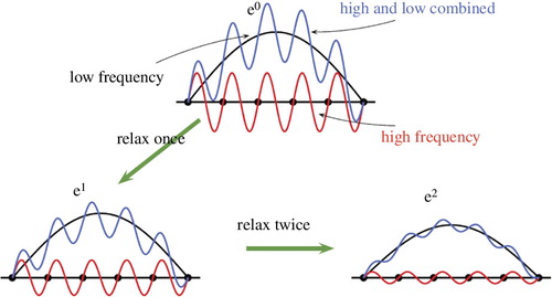
Traditional relaxation methods, such as Jacobi, Gauss-Seidel or SOR, have a common property called a ‘smoothing property’. This property makes such methods very effective at eliminating the high-frequency or oscillatory components of the error, while leaving the low-frequency or less oscillatory components relatively unchanged (Fig. 1). The convergence speed of general iterative methods depends mainly on the long wavelength error convergence, which means that these methods have a correct solution from the dense (short wavelength) structure but the convergence depends on the coarse (long wavelength) structure. One way to improve such a relaxation scheme, at least in the early stages, is to use a good initial guess. However, it is not straightforward to find a good initial guess for each problem.

Fig. 1 The smoothing property.

We introduce an MG that is suitable for overcoming the above problems. The MG is one of the most efficient iterative methods for solving elliptic PDEs on structured grids, and it is known to be effective in solving many other algebraic equations. The method exploits the smoothing property of traditional relaxation schemes together with the hierarchy of grids. Sometimes multigrid indicates one of the types of grid structures (also called ‘a nested grid’) in which several grids of different sizes are nested in a given domain, but in this paper we use the word ‘multigrid method’ to indicate an iterative method.

2.1. Basic two grid algorithm

Let Au=f be a system of linear equations. We use u to denote the exact solution of the system and v to denote an approximation to the exact solution, which is generated by some iterative methods. Then, the algebraic error is given simply by and the residual is given as follows.

For the convenience of presentations, assume and let . We assume is partitioned by uniform 2 ^k ×2 ^k rectangular grids, denoted by . We associate u and v with a particular grid, say . In this case, the notation u ^h and v ^h will be used. We first consider two grids, and .

We have already mentioned that relaxation schemes eliminate the error of smooth mode slowly. The MG is used to overcome this phenomenon by projecting the smooth mode error to a coarser grid(s) to approximate the long-wave error components. (It is illustrated in section 3.) The important point of using the coarser grids is that the smooth mode on a fine grid looks less smooth on coarse grids. Then, we use the following two strategies.

The first strategy incorporates the idea of using coarse grids to obtain an initial guess cheaply (nested iteration). The initial guess on the fine grid is the solution obtained by relaxing of Au=f on the coarse grid.

The second strategy incorporates the idea of using the residual equation to relax the error on the coarse grid. The procedure is described as follows.

Algorithm 1: A two-grid algorithm

1. Relax by Jacobi or Gauss-Seidel method

2. Calculate residual on the fine grid

3. Restrict : A ^h , r ^h onto the coarser grid

4. Solve the error equation: on

5. Interpolate : :

6. Correct the fine grid approximation:

The relaxation scheme reduces the Fourier components of short wavelength errors. The effect of a relaxation scheme depends on the boundary conditions and geometry of the grids, so there is no standard method. Typical relaxation schemes used to solve elliptic PDEs on a rectangular domain are Gauss-Seidel and Jacobi methods. A linear/bilinear interpolation is used for the prolongation, and the restriction operator is usually the transpose of a prolongation but a different operator can be used.

2.2. A multigrid algorithm

The two grid algorithm above can be extended to the multigrid case using several nested grids and repeating the correction processes on coarser grids until a direct solution of the residual equation is feasible. As we can infer from the two grid algorithm, basic elements of the multigrid algorithm are as follows.

• Nested iteration: Use several nested grids

• Relaxation: Use efficient methods to eliminate an oscillatory error on each grid

• Residual equation: Compute the errors on nested grids using the residual only

• Prolongation and Restriction: Data communications from a coarse grid to the finer grid and vice versa.

The simplest multigrid algorithm is a V-cycle which is described in Algorithm 2. For simplicity, we write u ^k , v ^k , f ^k , , and so on for , , and .

Algorithm 2: V-cycle recursive algorithm

1. Relax times with an initial guess u ^k .

2. If k=1 (the coarsest grid), then solve .

  Else,

3. Correct .

4. Relax times.

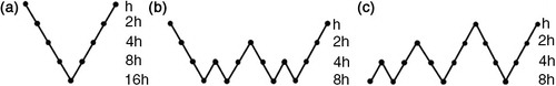
If the (*) part in step 2 of Algorithm 2 is computed twice, it is called a W-cycle. If the cycle starts from the coarsest grid to compute an initial guess and perform the V-cycle again with this initial guess, it is called the full multigrid V-cycle (FMV-cycle) (Fig. 2). For most problems, suffices. In the application of the MG with several nested grids, the coarsest grid has to be reasonably fine so that it can match the boundary conditions, that is, if the grid is too coarse, the computational boundary and the real boundary may be too far apart. In this case, the approximate solution converges slowly.

Fig. 2 Schedule of grids for (a) V-cycle, (b) W-cycle and (c) FMV-cycle.

3. MGs for the minimisation process in increment 3D-Var

In section 1, we already mentioned that the minimisation procedure of the 3D-Var finds the stationary point where the gradient of the cost function equals zero. In this study, we use the 3D-Var as the data assimilation technique. Then, the cost function J of the observational data and background data is defined as follows (Baker et al., 2003; Baker and Xiao et al., 2003).1

Here, the superscript b denotes the background value and superscript o denotes the observational data. T denotes the transpose matrix of a given matrix. B is a covariance matrix of background errors and R is a covariance matrix of observation errors, H is an observation operator. Usually, the model space and observation space are different and the variables are not the same. Hence, the operator H plays the role of interpolation and variable transform to compare the background values and observation values.

In many operational data assimilation systems, the incremental 3D-Var form is used instead of eq. (1).2

where δ denotes an increment of the variable, H denotes a linearised operator of the non-linear operator H and is called an innovation vector. The gradient of the cost function [eq. (2)] is given as follows:3

In the data assimilation system, a covariance matrix of background errors B is needed to determine the spatial spreading of observational information. However it is well known that an analysis field at different locations may have different correlation scales, which are difficult to estimate. Therefore, a traditional 3D-Var uses either correlation scales or recursive filters for representing B as follows (Xie et al., 2010).4

Here, U _h denotes a horizontal transform via recursive filters (or power spectrum) when the forecast area is a regional (or global) area. U _v denotes a vertical transform via empirical orthogonal function and U _p denotes a physical transform depending on the choice of the analysis control variable. Then by eq. (4), eq. (2) and (3) are written as follows. Let . By substituting eq. (4) into eq. (2) and eq. (3), we get the following.5 6

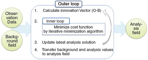
The data assimilation procedure of 3D-Var using the above cost function is as follows. The first step computes the differences between observations and the observation-equivalent values of background with the aid of the observation operator H to transform the model space to the observation space. The second step finds analysis increments that minimise the cost function based on the iterative minimisation algorithm. The analysis increments are updated at each iteration called the inner loop, and the analysis increments of the final iteration are added to the background to obtain the analysis field (Fig. 3).

Fig. 3 The minimisation procedure of the incremental 3D-Var.

3.1. MGs for the minimisation process

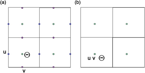
The numerical methods to calculate the minimum value of the cost function in the inner loop stage are usually iterative methods since the system is large and sparse. For example, the CG method is used in the KMA WRF model. To apply the multigrid as an iterative minimisation method of the inner loop, we solve the following equation on the uniform grid with data located at the cell centre (Fig. 4b).7 8 9

Fig. 4 The horizontal grid structures of WRF. (a) WRF model: Arakawa C-grid staggering, (b) WRF-Var: unstaggered Arakawa A-grid.

Then this system can be put in the following form:10

where

Equation (10) is defined on the grid of a data assimilation system. Unlike other iterative methods, the MG requires A and f defined on each of the coarser grids. (In particular, explicit entries or at least diagonals of A are needed.) These entries can be generated using a sequence of nested grids as follows:

Let denote a grid with a 2 ^k ×2 ^k (or its multiple) rectangular grids. Then, A and f are defined as follows on each grid of level k.11 12

Here the observation data, background data, background error covariance and observation error covariance are determined on each grid level. The details are described in section 3.2.

3.2. Basic components of the multigrid algorithm

In this subsection, we construct the MG for incremental 3D-Var based on CCFD. To do this, we consider the grid structure of the data assimilation system first. After determining the grid structure, the next step constructs the prolongation and restriction, relaxation and data processing in nested iteration, and so on.

3.2.1. Grid composition.

From here and thereafter we apply the MG on the 2-dimensional (2-D) horizontal space with the exception of the vertical direction. We assume that the shape of the horizontal domain is a square with the same grid spacing along the x-axis and y-axis. We also assume that the horizontal grid is an unstaggered Arakawa A-grid in which we assume all the variables are at the cell-centres, and the spatial discretisation method is the cell-centred finite difference method. Under these assumptions, we apply the MG for CCFD suggested in Kwak (1999).

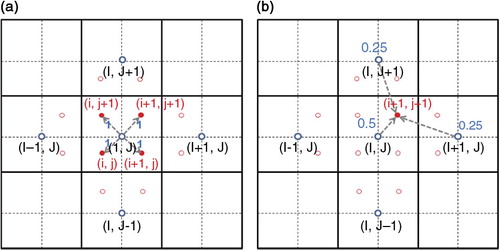
3.2.2. Prolongation and restriction.

To move vectors from the coarse grid to the fine grid, and from the fine grid to the coarse grid, we need so-called ‘intergrid transfer functions’. These are called a prolongation operator and a restriction operator in the multigrid community. In this paper, we use two types of operators as a prolongation operator, a simple prolongation (Fig. 5a) introduced by Bramble et al. (1996) and a weighted prolongation (Fig. 5b) introduced by Kwak (1999). A restriction is the transpose of each prolongation. The theoretical convergence of each scheme was verified by Bramble et al. (1996) and Kwak (1999).

Fig. 5 (a) Non-weighted prolongation for CCFD, (b) weighted prolongation for CCFD.

3.2.3. Nested iteration.

A nested iteration is a process that repeatedly computes and transfers data among geometrically nested grids. To define this process, we need a fixed ratio between a fine grid and a coarse grid. Usually, the ratio stands 1:2; the coarsest grid depends on the scale of a given model and a boundary condition. For instance, in the WRF regional model, one must have at least 20×20 horizontal grid points to predict an East-Asia area.

The data necessary to carry out the nested iterations on multiple grids are collected as follows:

• Observation data: Use the same data as the fine grid on every grid level.

• Background values: Use a bilinear interpolation to generate data on each level.

• Background error covariance (B): Generate it using the normal distribution on each grid level.

• Observation error covariance (R): Assume that R is a diagonal matrix having the same diagonal elements on every level grid.

3.2.4. Relaxation.

The relaxation scheme is one of the most important ingredients of the MG. The relaxation scheme is used on each grid to smooth the error by reducing the high-wavenumber error components. The relaxation scheme is a problem-dependent part of the MG and has the largest impact on overall efficiency. Some simple relaxation schemes are iterative methods such as the Jacobi method, Gauss-Seidel method or Richardson method.

It is well known that for the Poisson problem, the Gauss-Seidel method is more efficient than the Jacobi method, as the Gauss-Seidel method replaces the old value by a new value immediately after calculation. Thus, Gauss-Seidel converges faster to the solution than Jacobi as a single solver for the Poisson problem. However, the matrix arising from the minimisation problem of data assimilation is not explicitly given; instead it is given as the product of several matrices. Thus, it is hard to apply the Gauss-Seidel, since we have to know the individual entries of the total matrix. Therefore, we use the Jacobi (or damped Jacobi) method described below as a relaxation scheme for the minimising process.

The damped Jacobi method with a proper damping factor converges faster than the Jacobi method. Here, D is a diagonal matrix of A which can be easily computed by the formula:

(1) Compute , where is the standard basis vector

(2) Compute

(3) Set

In this relaxation process, parallel processing could be easily applied, which is another advantage of Jacobi.

Remark

(1) In this application of multigrid algorithms, we assumed that the domain is partitioned into 2 ^k ×2 ^k squares, but our MG can be applied to any rectangular region as long as we design an appropriate restriction and prolongation.

(2) In this study, so far we used the MG only for the efficient computation in the inner loop. However, we can use a similar technique for different resolutions in the outer loop. Some nontrivial work will be necessary because, in general, the outer loop is nonlinear. This is left for our future research.

4. Numerical example

4.1. Experiment 1

In the first idealised experiment, 2-D (surface) temperature data fields were constructed, and the temperature data are plotted in Fig. 6 with randomly distributed 179 surface temperature data items. The assumptions for this experiment are as follows. The background error covariance B is a normal distribution, and the observation error covariance R is an identity matrix. The given domain scale is 10 km×10 km with a maximum grid level 4(16×16) and minimum grid level 2(4×4) and we use the V-cycle MG. The observation operator is the composite of bi-linear interpolation and identity function.

Fig. 6 (a) The observation data, (b) the contour of observation data, (c) the analysis field of 3D-Var with the conjugate gradient method and (d) the analysis field of 3D-Var with the multigrid method.

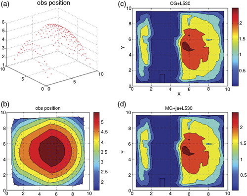
Under these conditions, we compare the iteration numbers of the CG method and that of the multigrid V-cycle with one pre-smoothing and one post-smoothing. For both algorithms, we stopped the iteration when the residual was less than 10⁻⁸. We see that the multigrid (V-cycle) converges to the approximate solution with fewer iterations than the CG method (Table 1). However, we see that the analysis fields of 3D-Var obtained by the MG is just the same as the analysis fields obtained by the CG method (Fig. 6).

Table 1. The result of numerical experiment 1

Number of iteration	CG ∇J	Number of iteration	MG ∇J
0	30.62536518	0	30.62536518
1	1.13541607	1	0.09419015
2	0.12427868	2	0.00038469
3	0.01349091	3	0.00000164
4	0.00160986	4	0.00000001
5	0.00020118	5	0.00000000
6	0.00002659
7	0.00000337
8	0.00000042
9	0.00000005
10	0.00000001
11	0.00000000

4.2. Experiment 2

For the second experiment, again 2-D (surface) temperature data fields were used as plotted in Fig. 7 with randomly distributed 179 surface temperature data items. In this experiment the data had more diverse wave-lengths than in the first experiment. The other conditions were the same as in the first experiment. Again, the multigrid (V-cycle) converged to the approximate solution with fewer iterations than the CG method (Table 2). We see that the analysis fields of 3D-Var by both methods are almost the same after the residual fell below the tolerance (Fig. 8). However, there were differences in some areas during the iterations (see Fig. 8a and 8d). The one V-cycle multigrid iteration already shows correct field on the right top corner where the data are sparsely observed while the CG method needed seven iterations.

Fig. 7 (a) The true state of temperature, (b) the contour of true data, (c) the observation data and (d) the contour of observation data.

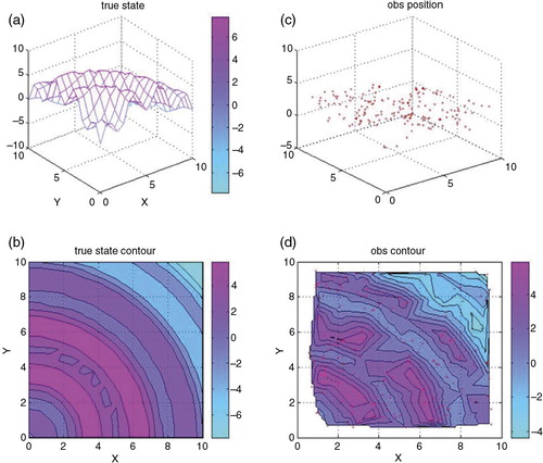
Fig. 8 (a–c): The analysis fields of 3D-Var with the conjugate gradient method at each iterative step 1(a), 7(b), and 13(c), (d–f): The analysis fields of 3D-Var with the multigrid method at each iterative step 1(d), 3(e) and 5(f).

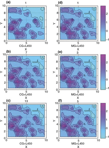
Table 2. The result of numerical experiment 2

Number of iteration	CG ∇J	Number of iteration	MG ∇J
0	20.43552705	0	20.43552705
1	2.64095750	1	0.06380830
2	0.41885882	2	0.00026161
3	0.06872520	3	0.00000117
4	0.01019913	4	0.00000001
5	0.00176452	5	0.00000000
6	0.00031169
7	0.00005252
8	0.00000787
9	0.00000138
10	0.00000020
11	0.00000003
12	0.00000001
13	0.00000000

Now let us compare the performances of the methods. The computation was performed on a window based notebook PC. No parallelisation was used. Let us count the total computational costs. One iteration of the V-cycle multigrid algorithm requires one pre-smoothing, one matrix-vector multiplication, one post-smoothing and two vector addition/subtraction. Finally, there is data transfer between grids. Altogether, it costs (roughly) three matrix-vector multiplication, two vector addition/subtraction and data transfer between grids.

Each iteration of the CG method requires (roughly) one matrix-vector multiplication, four inner product of vectors, two addition/subtraction. A rough comparison shows one multigrid V-cycle takes about two to three iterations of the CG method. Our numerical experiment shows that the V-cycle multigrid takes four iterations while the CG takes 10–12 iterations. Thus the total cost of the MG seems comparable with that of CG. However, there is some room to improve the MG; for example, using different smoothers or changing damping factors. There are also other variations, such as a W-cycle and FMV, which is known to be slightly better in practice. Still, a fair comparison would not be easy. It would be interesting if someone could implement the multigrid algorithm to solve real-life problems on parallel machines with various smoothers.

5. Conclusion

In this study, we introduced the MG for the minimisation process in data assimilation by interpreting the minimisation process as a numerical PDE discretised by the CCFD. We designed the prolongation and restriction operators based on this observation. We performed some numerical experiments and compared them with the CG method. We see that the MG has fewer iterations than the CG method and converges faster on the data-sparse area. A generalisation of our multigrid algorithm for other data such as wind field in 3-D space is left for our future research.

6. Acknowledgements

We thank the anonymous referees who gave many helpful comments to improve the quality of the manuscript. This work partially supported by the Korea Meteorological Administration.

References

- Baker D. M. , Huang W. , Guo Y.-R. , Bourgeois A . A Three-Dimensional Variational (3DVAR) Data Assimilation System for Use with MM5.
- Baker D. M. , Huang W. , Guo Y.-R. , Bourgeois A. J. , Xiao Q. N . A three-dimensional variational data assimilation system for use with MM5: implementation and initial results. Mon. Weather Rev. 2003; 132: 897–914.
- Bouttier F. , Courtier P . Data assimilation concepts and methods. Meteorol. Train. Course Lect. Ser. 2002; 117: 279–285.
- Bramble J. H. , Ewing R. E. , Pasciak J. E. , Shen J . The analysis of multigrid algorithms for cell centered finite difference methods. Adv. Comput. Math. 1996; 5: 1–34.
- Briggs W. L. , Henson V. E. , McCormick S. F . A Multigrid Tutorial. 2000; SIAM, Philadelphia, USA. 2nd ed.
- Downton R. A. , Bell R. S . The impact of analysis differences in a medium-range forecast. Meteorol. Mag. 1998; 117: 279–285.
- Gratton S. , Tointc P. L. , Tshimangaa J . Conjugate gradients versus multigrid solvers for diffusion-based correlation models in data assimilation. Q. J. Roy. Meteorol. Soc. 2013; 139: 1481–1487.
- Kwak D. Y . V-cycle multigrid for cell-centered finite differences. SIAM J. Sci. Comput. 1999; 21(2): 552–564.
- Li W. , Xie Y. , Deng S.-M. , Wang Q . Application of the multigrid method to the two-dimensional Doppler radar radial velocity data assimilation. J. Atmos. Ocean. Technol. 2010; 27: 319–332.
- Li W. , Xie Y. , He Z. , Han G. , Liu K. , co-authors . Application of the multigrid data assimilation scheme to the China seas temperature forecast. J. Atmos. Ocean. Technol. 2008; 25: 2106–2116.
- Richardson D . The relative effect of model and analysis differences on ECMWF and UKMO operational forecasts. Proceedings of the ECMWF Workshop on Predictability, ECMWF. 1998; Reading, UK: Shinfield Park. 20–22 October 1997.
- Xie Y. , Koch S. , McGinley J. , Albers S. , Bieringer P. E. , co-authors . A space-time multiscale analysis system: a sequential variational analysis approach. Mon. Weather. Rev. 2010; 139: 1124–1240.
- Zou X. , Vandenberghe F. , Pondeca M. , Kuo Y.-H . Introduction to Adjoint Techniques and the MM5 Adjoint Modeling System. 1997; NCAR Technical Note 435. Online at: www.rap.ucar.edu/staff/vandenb/publis/TN435.pdf .