An overview and illustration of sensitivity of forecasts with respect to initial conditions

Abstract

Sensitivity of forecasts with respect to initial conditions is an intermediate step in studies dealing with the impact of features in the initial conditions, or of observations in a data assimilation system, on the quality of the forecast. The sensitivity diagnostics however are obtained as approximations, and various formulations have been proposed over recent years. Since the sensitivity is assessed by computing a distance measure, the corresponding cost function can be estimated by a Taylor expansion. More recently, quadrature formulations have also been proposed. In this paper, these two approaches are re-assessed and attention is paid to specific assumptions made in those developments: the sometimes conflicting use of assumptions of linearity, the way non-linear aspects are taken into account and the relative formal merits of each technique. The presence, omission or absence of the second-order model derivative is also addressed. Eventually, a proposal for extending sensitivity diagnostics in a non-linear iterative context is made. The various diagnostics are illustrated and discussed in the framework of the Lorenz 96 toy model, for which both the first- and second-order model derivatives have been implemented. Several initial condition states are obtained by the means of a four-dimensional variational assimilation (4D-Var) algorithm. The sensitivity diagnostics are presented with respect to the observed dynamical model regime as verification time, beyond the assimilation window, is increased: respectively for a quasi-linear, a weakly non-linear and an early-phase, starting non-linear regime. The numerical results suggest that quadrature-based approximations of cost function reduction are more robust than Taylor-expansion-based ones. Furthermore, the quadrature-based diagnostics do not require the usual omission or simplification of high-order derivatives. A straightforward extension to an iterative context also is possible and illustrated.

• four-dimensional variational assimilation
• forecast sensitivity to initial conditions
• quadrature estimates
• Lorenz 96 model

1. Introduction

This note focuses on recently published material about observational sensitivity computations in a data assimilation system. The focus is however kept on the sensitivity to the initial conditions, and the steps for extending the sensitivity analysis towards observations are not taken here. What is kept is the framework of a data assimilation algorithm, for computing the variations of initial conditions by the means of analysis increments. The sensitivity of a forecast to the initial conditions is defined as a distance measure of the forecast state with respect to a verifying state:1 where C is a symmetric, positive definite matrix and x ^f and x ^t stand for the test forecast and the verifying state, respectively. Various recent papers have introduced this definition or a similar one, like Langland and Baker (2004, hereafter LB04) and Errico (2007, hereafter E07). Both LB04 and E07 are now reference papers for applied sensitivity studies in real numerical weather prediction (NWP) and assimilation systems (Gelaro et al., 2010, or observation impact studies for the CONCORDIASI field campaign, Nathalie Saint-Ramond and colleagues, personal communication). The sensitivity analysis consists then in assessing which features in the initial condition, if modified, would bring a significant reduction in the function e. Or, put in different words, which features, if changed, would bring a benefit in the quality of the forecast as compared to the verification data. Thus, a key aspect in sensitivity analyses is to be able to compute the reduction δe, which is not in general available exactly. Daescu and Todling (2009, hereafter DT09) performed an overview of various methods of approximation of the forecast distance reduction, by separating them into two families based on either Taylor expansions or quadrature formulations. Their proposal of quadrature formulations is a more novel aspect for sensitivity computations in the NWP context, though DT09 demonstrate for instance that LB04's method actually is one case of a quadrature approximation.

In Section 2 of this note, the two families of approximation of the forecast distance reduction are studied. The sensitivity analysis performed by E07 is re-assessed with a focus on two critical steps, namely the assumption of a linear evolution of the perturbation and the substitution of the second-order model derivative by a difference of two first-order model derivatives. Furthermore, the quadrature-based sensitivity formulations introduced by DT09 are discussed. Finally, in Section 2, sensitivity diagnostics for iterative processes are proposed. These expressions seem consistent with iterative non-linear assimilation algorithms, and bear similarities with the proposals made by Trémolet (2008).

The various sensitivity diagnostics are illustrated and compared in the framework of the Lorenz 96 (Lorenz, 1996, hereafter L96) toy model (Section 3). A four-dimensional variational assimilation (4D-Var) is used as a tool for computing the variations of the initial conditions. The 4D-Var benefits from observations over a time window [t ₀, t ₁]. The forecast verification period is considered to start after this assimilation period (t _v ≥t ₁). Because the accuracy of the sensitivity formulas depends on the order of magnitude of errors and the importance of non-linear model features, the results are interpreted in terms of dynamical model regime for perturbation growth. A separation is made between quasi-linear, weakly non-linear and early-phase non-linear behaviour, as the verification forecast range t _v is extended. The results are summarized in Section 4.

2. Considerations on sensitivity computations

2.1. A Taylor expansion-based case: Errico (2007)

As a first step, the sensitivity calculations based on Taylor expansions, as presented in Errico (2007, E07), are re-derived and discussed. E07 handles the forecast error measure e(x ^f ) using the summation along individual components of the state vectors:2 where c _ij are the elements of matrix C. The sensitivity analysis in E07 consists in developing the Taylor expansion of e with respect to a small change in the initial condition x ⁰. The forecast state x ^f is, in the general case, obtained by integrating a model M: x ^f =M(x ⁰) where M is a full, non-linear forecast model. Eventually, we look for appropriate estimates for the variation δe(δx ⁰)=e(M(x ⁰+δx ⁰))−e(M(x ⁰)). The first-order term of the Taylor expansion of δe is obtained by introducing the resolvent model, denoted M. M is by definition the tangent linear model integrated in time. The tangent linear model is obtained by a linearization of the full model M along a trajectory defined as the forecast started from x ⁰. The resolvent model can be represented by a matrix of coefficients m _ij , thus leading to the following expression, which corresponds to eq. (6) of E07:3 With these notations, the first-order derivative of e with respect to any coordinate of the initial perturbation is readily obtained:4 which corresponds to eq. (7) in E07. Equation (4) provides the vector 2M ^T C(x ^f −x ^t ) and thus:5 is the first-order variation of measure e with respect to δx ⁰. This relation corresponds to eq. (14) of E07.

The variation of e may be extended to order two, which then provides the term δe ₂ of E07. The second-order derivative of M can be obtained by a further derivation of eq. (4) with respect to a second component of the initial perturbation vector:6

This is eq. (8) in E07. We now write for the sake of simplicity:7

The first term in the expression of δe ₂ simply is δe ₁. After some rearrangements using eq. (6), reads:8

The first term comes from the first-order variation [refer to eq. (4)] while the second and third terms above come from the second-order variation [see eq. (6)]. After rearrangements, also reads:9

At this stage, E07 uses the following simplifying assumption [this is eq. (6) in E07]:10

To be more specific, it is assumed that the linear integration term , for any component j, is a fair estimate of the final forecast difference . This partial assumption of linearity of the forecast model is in principle questionable, since it is otherwise assumed that the forecast model M is non-linear, so that it should be worth to extend and analyse its Taylor expansion beyond order one. Moreover, this assumption is stated all along the model integration from t ₀, the initial time, through t _v , the verifying time, since the substitution is performed at verifying time. We also note that this replacement is first-order accurate with respect to δx ⁰ for the non-linear model M, since it also can be interpreted as a truncation of the Taylor expansion of M at order two and above. Therefore, after substitution, the expressions following below for δe ₂ will be accurate at order two, because of the extra dot product with δx ₀ [see eq. (7)]. In other words, the error bounds for δe should be of order three with respect to δx ⁰. Continuing E07's derivation, we now introduce the analysis state with the superscript a and write: +. In terms of an assimilation system, x ^f is the forecast state obtained from an integration started with the background state x ^b while x ^af is the forecast state started from the analysis x ^a .

Back to δe ₂, we now can further rearrange its expression:11

Noting that:12 which is eq. (5) of E07, and reusing the partial assumption of linearity of the forecast model discussed previously:13 we can further write:14

Since δm _ik contains the derivatives of the resolvent with respect to the initial state components, we eventually obtain the following expression for δe ₂:15

This expression represents the second-order accurate variation of e in the lines of E07. It involves the second-order derivative of the forecast model, present in the bilinear term M ₂(δx ⁰,δx ⁰). This bilinear term also involves an integration along a trajectory, which is precisely the same as for the resolvent model, namely the non-linear forecast M(x⁰) started from x ⁰. The prevalence of this second-order model derivative is a well-known feature of sensitivity computations [see for instance in Le Dimet et al., 2002, or in Trémolet, 2008, his section 3.3]. It is in general ignored, since its computation is out of range in NWP systems.

To proceed further, E07 has substituted in the following way:16

By this substitution, the second-order model derivative disappears and is replaced by a perturbed model resolvent M+δ M which is interpreted as the resolvent matrix integrated along the trajectory started from the analysis x ^a , as opposed to the resolvent M which is integrated from the background initial condition x ^b (at verifying time: x ^f =M(x ^b ) and x ^af =M(x ^a )). Introducing the notations M _b = M and M _a =M+ δ M and substituting in the above relationships leads to:17

which is equivalent to eq. (17) of E07.

It is worth to stress here that the substitution of eq. (16) corresponds to a first-order approximation for the resolvent model. This assertion can be seen by the relationship: +, where M˜ is the resolvent along the trajectory started from x ⁰+δx ⁰. Indeed, M ₂(δx ⁰,δx ⁰) will by definition converge to the finite difference when δx ⁰ becomes infinitesimal. Thus, the substitution of eq. (16) is a new case of partial assumption of linearity of the forecast system, but the substitution now consists in replacing the (bi-)linear term by a (non-linear) finite difference. Therefore, this substitution has the opposite effect compared to the substitution in eq. (10) where high-order terms are removed. In this respect, the two substitutions are of conflicting nature and an error is in principle introduced. The substitution in eq. (16) again is taken to be valid all along the model integration from t ₀ through t _v . By construction, the error bound of this replacement in the non-linear forecast model formulation is of third order with respect to δx ⁰ (i.e. its precision is of second order). Thus, the substitution actually leads to a fourth-order error bound in δx ⁰ for δe ₂, as can be seen for instance with the left product by δx ⁰ in eq. (17).

In E07, the replacement of the second-order derivative by the perturbed resolvent model is an essential step for introducing the effect of a varying trajectory of linearization. As we have illustrated above, this interpretation is correct, but its derivation in E07 makes an explicit use of assumptions of quasi-linear behaviour for several simplifications [based on eqs. (10) and (16)] that do have opposite impacts in terms of accounting for or ignoring high-order terms. In addition, these assumptions of quasi-linear model behaviours must hold all along the time integration of the models (from t ₀ through t _v ), because the simplifying substitutions are done at verifying times. This aspect will be illustrated in Section 3. As an intermediate conclusion, the sensitivity formulations of first- and second-order given in E07 have been re-derived, with an emphasis on cornerstones of E07's developments. The presence of the second-order model derivative has been explicitly formulated. Those steps where some type of quasi-linear assumption is made, with conflicting effects on accounting for or discarding high-order terms, have been highlighted. These effects should not become sensitive at the same time, however, since they apply on error truncations of different order: the substitution in eq. (10) affects δe at order three (accuracy is second order) while the substitution in eq. (16) affects δe at order five (fourth-order accuracy). The first-order variation δe ₁ and the second-order variation δe ₂ of E07 are further illustrated for the L96 model (Lorenz, 1996) in Section 3.

2.2. Quadrature-based estimates of a forecast distance difference: Daescu and Todling (2009)

An alternative approach for the calculation of forecast distance sensitivities has been proposed by Daescu and Todling (2009, DT09). Besides Taylor expansion calculations, DT09 introduce a quadrature-based estimation by considering the variation δe=e(M(x ^a ))−e(M(x ^b )) as a parametric function along the segment [x ^b ,x ^a ]. The parameter is a single scalar s∈[0,1] such that any initial state x ⁰ on this segment can be defined as x ⁰=x ^b +s(x ^a –x ^b ). A new parametric distance function is then derived as: = and the change of e between background and analysis forecasts becomes:18

where the fundamental theorem of calculus is invoked. Several high-order approximations of the integral computation can be obtained, by using various quadrature estimates. Each estimate is based on a specific rule of approximation (Trapezoidal, midpoint, Simpson) and is associated with a specific formulation of its error bound. In particular, DT09 show that the term [(x ^f −x ^t ) ^T C M _b +(x ^af −x ^t ) ^T C M _a ](x ^a −x ^b ) corresponds to a numerical quadrature approximation of δe following the Trapezoidal rule. Furthermore, DT09 identify this expression with the sensitivity formulation proposed by Langland and Baker (2004, LB04). It is also worth to notice that this expression is based on two computations of the gradient of e with respect to the initial condition variable x ⁰, denoted g, respectively, at points x ^b and x ^a , and using as trajectory of linearization the forecast started from x ^b and x ^a , respectively. This assertion is demonstrated by the property: g(x ⁰) ^T =2(M(x ⁰)−x ^t ) ^T C with the resolvent model along the trajectory M(x ⁰). This relationship is valid at any point x ⁰ along the segment [x ^b ,x ^a ], and furthermore . Thus, an equivalent formulation for the Trapezoidal rule quadrature estimate, as first proposed by LB04, reads: δe _LB =1/2(g _b +g _a ) ^T (x ^a –x ^b ). Note also the close resemblance between the formulations of δe ₂ [eq. (17)] and δe _LB , with only a difference through swapping M _b with M _a . They are very similar, but not equivalent. DT09 use fundamental properties of integral calculus for single-variable functions to prove that the estimate is second-order accurate (the residual can be expressed as a third-order term in x ^a –x ^b ).

Several other alternative estimates of δe are proposed in DT09. The midpoint rule quadrature estimate is second-order accurate and reads:19

In eq. (19), the point is that the gradient is evaluated at the midpoint x ^mid =(x ^a +x ^b )/2. The resolvent accordingly is linearized along the trajectory M(x ^mid ). Simpson's rule quadrature estimate provides a fourth-order accurate formula:20

δe _Simp actually is readily computed if δe _LB and δe _mid are known, since it is a linear combination of both. An advantage of the quadrature-based estimates over Taylor-based formulations like in eq. (15) certainly is that no second-order model derivative M ₂ appears, since the accuracy of each formulation is obtained by computing and combining first-order gradients at prescribed positions. One possible drawback, conversely, is that the expressions and their error bounds in principle only hold for variations along the given segment [x ^b ,x ^a ]. We illustrate these various sensitivity formulas in the framework of the L96 (Lorenz, 1996) toy model in Section 3.

2.3. Varying trajectories of linearization as a result of an iterative process

Yet, other possibilities for addressing the dependency of sensitivity diagnostics with respect to the trajectory of linearization do exist. In the spirit of Taylor expansions, the trajectory is naturally provided by the integration of the non-linear model started from the reference initial condition. Successive small corrections of a given initial state provide then new Taylor expansions, and the associated sensitivity is obtained in iterative steps. Let us consider [x ⁰, x ¹,…,x ^m ] a set of such initial conditions, with and each δx ⁱ is a small variation. We consider each distance measure e ⁱ as the difference of the respective forecasts with a verifying state x ^t : = ; and the total variation .

Keeping only approximations at order one with respect to the small successive variations of the input δx ⁱ :21

In eq. (21), M _i−1 stands for the resolvent model linearized along the trajectory started from x ⁱ⁻¹. Thus, in this iterative process, the dependency of the sensitivity with respect to successively changing trajectories of linearization becomes visible through the cumulative terms added at each new loop. Such a sensitivity diagnostic might apply in the context of multiple analyses, where x ² would be a re-analysis with respect to x ¹. Another possible application of this approach is in a multi-incremental assimilation, where each x ⁱ⁺¹ is an iterative correction of the previous solution x ⁱ . Equation (21) bears similarities with the formulation of the first-order variation denoted I ₁ in Trémolet (2008), as is obtained by iteratively adding first-order contributions computed as simple vector multiplications. Each vector g _i is obtained by applying the adjoint model linearized along the trajectory started from x ⁱ⁻¹ to the iteratively forecasted departure (weighted by C). A difference in the derivation for eq. (21), with respect to Trémolet (2008), is that the data assimilation system itself has not been made explicit here, while Trémolet was interested in making the operators of the incremental assimilation process visible.

A second-order evaluation of the variation of e can be obtained by furthermore considering the square products between all first-order terms of the type , since e is quadratic. In addition, one also should take into consideration the terms involving the second-order model derivative, which is done here formally although these terms would not be accessible in an NWP context (these terms are provided in the framework of our toy model, for illustration, in Section 3). Omitting these terms, as discussed for eq. (15), is for instance done in Trémolet (2008) in the context of an NWP data assimilation system. In its complete form, the second-order term of the variation δe reads:22

leading to the second-order approximation of the variation of e at step m:23

Equation (23) bears similarities with the formulation of the second-order variation denoted I ₂ in Trémolet (2008), as is obtained by iteratively adding a second-order variation of the functional e to a corresponding first-order contribution. In Trémolet (2008), however, the functional e actually represents the distance function to the background state of the assimilation J _b and an explicit formulation involving the operators of the assimilation process is searched. Note that for m=1, if δx ⁰ is taken as the (single-step) analysis increment, then the RHS of eq. (23) is equivalent to eq. (29) in DT09. Note also that, at order one, is equivalent to eq. (27) in DT09 and eq. (14) in E07.

3. Results with the Lorenz 96 model

3.1. Description of the model implementation

The diagnostics of Section 2 are illustrated using the L96 toy model (Lorenz, 1996) with K=40 degrees of freedom. The non-linear evolution of the state reads:24

with the periodic boundary conditions: =. The timestep scheme is a fourth-order Runge-Kutta scheme, with a timestep dt=0.01. The forcing term F=8 is a usual value for this model, and means that a highly chaotic (non-linear) behaviour is chosen. The resolvent model is obtained by integrating the tangent linear equation. For the L96 model, the tangent linear model can be described by its Jacobian matrix representation. The j-th line of the Jacobian f then reads:25

where x ^traj stands for the state of the trajectory of linearization (or any of its individual components ). The non-zero values above span from column j–2 to column j+1. These elements are similar to, for instance, eq. (7) of Lorenz and Emanuel (1998). Periodic boundary conditions are applied in accordance with the non-linear version. The time integration of the resolvent model is obtained by a fourth-order approximate expansion of the matrix exponential formal definition of the resolvent ==+ where an integration from t ₀ to t ₁ is assumed.

The second-order model derivative can be represented as a series of elementary K×K (Hessian) matrices, which eventually compose the tensor representation of this model. The j-th ranked elementary matrix has zeroes everywhere except on four elements:26

The –1-values are located at the lines and columns (j−2, j−1) and (j−1, j−2); the 1-values are located at the lines and columns (j−1, j+1) and (j+1, j−1). Note that for the L96 model, because the non-linear terms are simple second-order cross products between individual elements of the state vector, the second-order derivative (tendency) does not explicitly depend on the trajectory x ^traj . This dependency however does exist for the second-order model derivative, because its time integration requires combinations with the resolvent model (see below, chain rule). For each elementary matrix, periodic boundary conditions are applied in accordance with the tangent linear and non-linear models. The time integration of the second-order model derivative is based on the chain rule: =.

The data assimilation system is a 4D-Var. The minimization is carried out by a conjugate gradient method.

The numerical results discussed in this note are obtained with the following experimental setup:

1. The truth is run over 40 d, where 1 d is defined as 20dt and is often considered as one “day” in the context of the L96 model. The initial condition is = plus a perturbation of F/1000 on X ₂₀. According to individual time series of various model points X _j , transient behaviour vanishes after about 13 d. In past studies, Lorenz and Emanuel (1998) used 90 d to ensure satisfactory convergence on the attractor; Yang and Delsole (2009) used about 375 d.

2. A background state x^b is defined at day 39, as the true state at this range plus a random perturbation of standard deviation σ_b applied on all elements of the state vector. This background state is the start of a background trajectory from day 39 through day 40. The value σ _b =0.2 is used in this study, which corresponds to a size of background errors about two orders of magnitude smaller than the variability of the L96 state (see for instance in Fig. 1).

3. Observations are defined for every second point (every odd valued position of the state vector), and for every 5dt in the assimilation window from day 39 through day 40 (5dt=0.05 is considered as a pseudo-6 hour time interval, as suggested in previous studies with L96). The observed values are defined as randomly perturbed values of the true state, with a standard deviation σ _o =0.2. The choice σ _o =σ _b =σ is always kept. Thus, a total amount of 5*20=100 observations is assimilated.

4. The background and observation error covariance matrices B and R are simple diagonal matrices with the constant values and , respectively. A consequence of this choice is that the assimilation system is specified to be optimal.

5. A total of 10 random occurrences of the above defined assimilation problem have been run successively,in order to assess the robustness of the results and interpretations in a more systematic manner. There is obviously a certain variability of the true distance function reduction δe over the set of realizations, but this variability is not of interest per se. When relevant, a mean percentage of difference between various sensitivity measures is displayed in the follow-on of this paper (see in Table 1).

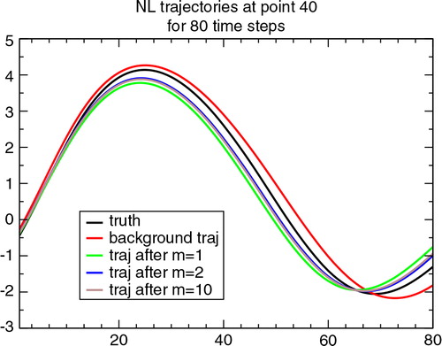
Fig. 1 Time series of L96-values at point j=40. Time t ₀=0dt corresponds to the start of the assimilation window; the end of the assimilation window is at t ₁=20dt; the final forecast range displayed is at t _f =80dt. The time unit is in model iterations. The black, red and brown curves, respectively, represent the trajectories computed from the truth, the background and the analysis states for run 1 out of the 10 random realizations when σ _o =σ _b =0.2. The green and blue curves show trajectories obtained during the non-linear minimization process for m=1,2, resp.

With these settings, the total cost function is fairly close to a quadratic function, and the conjugate gradient minimization has converged after m=10 iterations. The forecast models are assumed to be perfect, which means that the 4D-Var problem is of strong constraint type and model error is ignored.

3.2. Illustrations of sensitivity diagnostics

3.2.1. Aspects about various successive trajectory runs.

Figure 1 displays several L96 model integrations from time t ₀=0dt (day 39 of the truth run) through time =0.8 (day 43 of truth run) for point X₄₀. The forecasts started from the analysis (brown curve), the background (red) and the true state (black) are shown, along with two intermediate trajectories obtained in the course of the minimization. It is readily seen on Fig. 1 that all five trajectories remain very close in the first day of integration, from t₀ through t ₁=20dt=0.2. This period corresponds to the one where observations are assimilated. Beyond t ₁, the trajectories progressively diverge and after three more days of forecast, at time t _f, the dispersion between all five runs is of about one L96 model unit. The period [t ₁,t_f ] is considered to be the verification period, where the sensitivity diagnostics are evaluated and discussed.

Table 1. Values of the various sensitivity diagnostics evaluated at verification times t _v =40dt=0.4 and t _v =80dt=0.8 for the case when σ _o =σ _b =0.2. Incremental estimates for midpoint, Simpson, , and are given for m=10, and thus also correspond to the values for m=10, t _v =0.8 in Figure 2. The values are for one given occurrence out of the 10 random realizations (run 1). The mean relative error is with respect to the true reduction and averaged over all occurrences. It is given in percentages.

Type of	Run 1	%	Run 1	%
δe	t v =0.4	t v =0.4	t v =0.8	t v =0.8
δe 1	−6.96	177.55	−20.88	105.59
δe 2	−2.58	6.27	−11.40	10.64
δe LB	−2.52	4.50	−8.05	8.17
δe mid	−2.57	4.18	−10.53	3.67
δe Simp	−2.56	2.05	−9.70	1.73
	−2.60	4.43	−12.03	6.84
	−2.56	1.98	−9.80	1.77
	−10.57	253.01	−33.68	170.59
	−2.78	11.93	−14.91	23.93
	−2.51	1.65	−9.27	21.95
Truth	−2.64	—	−10.67	—

3.2.2. Interpretation in terms of the dynamical model regimes.

The dynamical regime of perturbation growth along the period [t ₀,t_f ] can be qualified for instance by checking the individual components that contribute to the Taylor expansion of the distance cost function reduction δe. Note that in this study, the norm C associated with e simply is taken as the canonical norm: . The formulations of eqs. (21) and (22) are taken as the basis. These formulations provide one first-order term, , and two second-order terms, and . In addition, one third-order and one fourth-order term are accessible since they are composed with the first- and second-order model derivatives only (third- or higher-order model derivatives have not been considered in this study):27

At time , the budget of δe is mostly given by (here, our reference value for m is after all 10 iterations have been collected, so m=10). Thus, only the first-order term and the square term of second order involving the resolvent model M, are significant. Terms , and are about 2–3 orders of magnitude smaller than and (among all 10 test runs). Because the higher than one-order model derivatives are negligible, the model behaviour at t=0.2 can be considered as quasi-linear.

At time t=40dt=0.4, the three extra non-linear terms , and only are 1–2 orders of magnitude smaller than and . The approximation provides an estimate of δe accurate to about [10–20%] only. The other three terms, involving the second-order model M ₂, are of about equal order of magnitude, and their sum is enough, in any of the 10 test runs, to obtain a total estimate of δe up to about [1–3%]. These values indicate that the second-order model derivative has a small but significant contribution, while higher (than two) order model derivatives are still negligible. Because of the relative magnitudes discussed above, this dynamical model behaviour can be considered as a weakly non-linear one.

The fact that the observed dynamical regime progressively shifts from quasi-linear to weakly non-linear between t _v =0.2 (1 d forecast range) and t _v =0.4 (2 d) is a consequence of the growth of the differences between the compared forecast states. The observed time range of this growth seems consistent with for instance the values of the leading Lyapunov exponent: Lorenz and Emanuel (1998) give 2.1 d, Carrassi et al. (2009) give about 3 d. Thus, differences of about 2.10⁻¹ between various states at t ₀, as prescribed when σ=0.2, would result in differences of about [0.5–1] after about 2 d. These estimates are in accordance with Fig. 1 and indicate that indeed, non-linear aspects should progressively become visible.

At time t=80dt=0.8, the truncated expansion (denoted ) does not provide anymore a highly reliable estimate of δe. Model non-linearities of high-order start to become significant. This aspect is seen from the increasing relative role played by the terms , and , whose relative ratios of absolute values with respect to and now are of about [0.2–0.4] in the test runs. Thus, t=0.8 can be considered as corresponding to the starting phase of the non-linear model regime.

3.2.3. Results in terms of sensitivity diagnostics.

As concerns the various diagnostic estimates of δe discussed in Section 2, a clear numerical distinction is seen in Table 1 between the first-order accurate approximations like δe ₁ (E07) and , and the second (or higher)-order accurate formulas (δe ₂ of E07, δe_LB of LB04, midpoint and Simpson's rules estimates of DT09, and ). The first-order terms are of opposite (negative) sign with respect to their (positive) second-order correction: compare δe ₁ with δe ₂–δe ₁ or with in Table 1 for t_v =0.4 and t_v =0.8. In absolute values, the first-order diagnostic terms are about twice as large (or even more) compared with the values of their second-order corrections. This property was found to be even more pronounced in experiments with σ=0.01, where the various forecasts of interest would be much closer one to another.

This particular feature is due to the quasi-linear or weakly non-linear model regime combined with the fact that background and analysis are relatively close to the true state in these experiments. Therefore, using the linearized approximation +, one may write:1

Here, the second and higher order model derivatives are omitted and only the dynamically predominant resolvent model is considered. The first term can be approximated with another linear assumption, by introducing the analysis error ε ^a so that:

By substitution and a further linearization:

Eventually, an approximate relation for − is obtained, involving only the dynamically predominant resolvent model:

The first scalar term is derived from the first-order variation of δe, and it is equal to minus two times the second-order-derived contribution (second scalar term), up to an additive correction depending on the orthogonality of with . Trémolet (2007) showed that the equality is exact when the model is linear and the forecast minimizes the distance cost function e. Indeed, under these assumptions, it can be shown that . Similar proportions in sensitivity results were furthermore obtained with the GEOS-5 system in Gelaro et al. (2007), with an atmospheric data assimilation system. As a numerical consequence, the first-order estimates of δe exhibit relative errors of about 100% or more at t _v =0.4 and t _v =0.8.

At verification time t _v =0.4 (left side columns in Table 1), differences between the various diagnostic formulas are seen when the numerical values are checked in more detail. Thus, provides an estimate which is of slightly poorer average quality than δe ₂ (E07), δe _LB (LB04) or the midpoint/Simpson's rule quadrature estimates (DT09). A significantly better estimate is obtained when the two extra terms, that can be computed because M ₂ is available in this toy model, are added (+ in Table 1). This result is consistent with our definition of a weakly non-linear model regime: for the extended estimate , the extra high-order aspects that count in the Taylor expansion of δe are those that are derived using both the first-order (Jacobian/tangent linear, or adjoint) and second-order (Hessian) model derivatives.

For (right side columns in Table 1), the incremental estimates are of clearly poorer quality than the simple ones. This deterioration is due to cumulated errors with iterations m, because of the missing higher than two-order terms (or higher than one-order terms for F ₁ ^m ). Remember that this forecast range is in the start phase where non-linearities become significantly sensitive. It is nevertheless worth noticing that the Simpson's rule estimate outperforms any other approximation for δ _e .

In the formula for δe ₂ of E07, the substitution of the bilinear integration by a finite difference of the resolvent model (which we called a ‘partial assumption of linearity’ in Section 2) implicitly allows us to take into account some weakly non-linear behaviour of higher order. In the cases of LB04 and the other quadrature estimates of DT09, the non-linear effects remain present since no truncated development in a Taylor expansion sense is performed. As introduced in DT09 and re-discussed in Section 2, diagnostics like δe _LB (LB04), δe _mid (midpoint rule quadrature) and δe _Simp (Simpson's rule quadrature) are obtained by recomputation of gradients and their combination. In this process, the trajectory of linearization has to be adapted and chosen as the forecast started from a given initial state (background, analysis, their midpoint, in these cases). The major ingredient for a fourth-order estimate in the Taylor expansion-based diagnostic term is the inclusion of higher order model derivatives. In the context of the present toy model study, these higher order terms are those that are accessible through the availability of the Hessian of the dynamical system, leading to the extended formula of .

In quadrature-based diagnostics, the number of recomputations basically controls the accuracy of the estimate: δe _LB combines two gradient informations computed using the background and the analysis, and is second-order accurate; δe _mid is based on one recomputation only at midpoint position = and also is second-order accurate; is based on three gradients and is fourth-order accurate. The toy model results, for rather weakly non-linear conditions, show that the Simpson's rule quadrature indeed provides estimates which on average are more robust and accurate than the other tested diagnostics. Only as long as non-linearities remain significantly weak, do some other sensitivity formulas propose comparable alternatives, in particular δe _LB , δe _mid and .

For verification times that would lie within the more settled non-linear regime (t>0.8 or other experiments not shown here), the Simpson's rule quadrature approximation provides the most acceptable values. Checking directly the form of the function for various values of s (with a step of 0.1), it turns out that this cost function is monotonously decreasing along the interval [0,1] in most cases where the quadrature-based estimates still provide acceptable values (not shown). On the opposite, the piecewise values of indicate that this function possesses multiple maxima/minima in those cases where for instance the Simpson's rule quadrature fails. This finding is consistent with increased values of higher order derivatives, leading to an inflation of the error bounds for the quadrature-based estimates. This practical result nevertheless suggests that quadrature estimates could be robust over a certain range of verification forecast times, for various dynamical and assimilation systems possibly of the complexity of atmospheric NWP systems. This finding is in line with the practical application of these diagnostics given in Section 4 of DT09 (with the GEOS-5 system of NCEP and NASA/GMAO).

3.2.4. Illustration of the sensitivity diagnostics with iteratively changing trajectories of linearization.

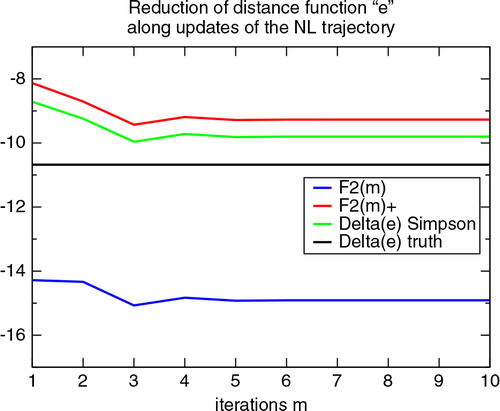
Finally, Fig. 2 displays values of , and δe_Simp for (, ), with respect to the iterates m of trajectory recomputations. For and , the incremental formulation is embedded in their definition [see eqs. (21–23)]. For , each successive couple of initial and final states is considered to define one segment over which the quadrature approximation is evaluated. Then, like for and , the successive estimates of are summed. In this stepwise estimation of the quadrature approximation of δe, the precision of each individual approximation should lie within the theoretical error bound of the respective quadrature (for Simpson's rule, fourth order). Thus, the iterative sum is expected to provide an estimate of the total reduction that has a comparable error with the single-step estimate computed in one go over the interval , except if errors add up. This numerical behaviour is indeed observed, both for δe_mid and δe_Simp , at and (see in Fig. 2 and in Table 1). However, for , the iterative estimates perform significantly poorer than their one-go counterparts (see in Table 1). For the term , the accumulation of error is related to the term which is positive and tends to bring a too large contribution to the total. Here, extra non-linear terms that could counter-balance this contribution are missing when the model regime starts to leave the weakly non-linear phase.

Fig. 2 Successive values of the cumulative variations , and DT09's Simpson rule quadrature estimate, for the 10 successive loops m=1,10 when σ _o =σ _b =0.2 (blue, red, green, resp.). The curves are for run 1 of the 10 random occurrences of the assimilation problem. Verification time is t _v =80dt=0.8.

Figure 2 nevertheless illustrates a practical possibility to evaluate the impact of a changing reference trajectory when computing a sensitivity diagnostic based on either a Taylor series (and truncation) or a quadrature estimate, in the context of an iterative correction process. In the case of Fig. 2, the first two iterations are those that drive the solution closest to the minimum, among all minimization steps. Accordingly, the largest amount of reduction for the forecast distance measure is obtained in the first two loops m=1,2. The next loops provide fairly negligible contributions. These results are consistent with the observed reduction of the total cost function J with each iteration in the non-linear minimization (not shown). Figure 2 illustrates that the iterative estimates provide a consistent picture of how the progressively adjusting trajectory allows one to capture, little by little, a fairly good estimate of the true reduction, even in a weakly non-linear model regime. In the case of the δe _Simp -diagnostic, the panel also illustrates the difference that has to be made between the (three) different trajectories used to compute the diagnostic itself and the (ten) different trajectories obtained in the non-linear minimization process.

4. Conclusions

In this paper, we have readdressed sensitivity diagnostics recently proposed in Errico (2007, E07) and Daescu and Todling (2009, DT09). In particular, we have shown that the formula δe ₂ in E07 is obtained after two crucial steps of quasi-linear assumptions: (1) when considering that the non-linear forecast can be approximated by a linear one for some terms, and (2) when approximating the second-order model derivative by a finite difference of two model resolvents integrated along slightly differing trajectories. The first substitution is in contradiction with considering higher order variations for the sensitivity analysis in a non-linear system. It nevertheless allows one to continue the developments, with an overall second-order accuracy for the distance measure reduction δe. The second substitution has an opposite effect to the previous one, since it consists of reintroducing higher order dynamical behaviour in the approximate diagnostic. It is otherwise within the bounds of fourth-order precision for δe, thus not too problematic as long as the model regime is quasi-linear. Nevertheless, these two conflicting assumptions should be considered as a theoretical weakness of formulas like E07's δe ₂.

DT09 have proposed sensitivity formulations for δe that only require multiple trajectory and gradient recomputations. Quadrature formulations, considering the distance measure e as a single parameter functional on the segment , are then invoked to obtain second-, fourth-, or higher-order estimates. In contrast to Taylor expansion-based sensitivity approximations like E07's, where the second-order model derivative does quite naturally appear, the absence of this or higher order derivative terms in quadrature-based approximations is an advantage. Indeed, high-order model derivatives require extra model configurations to be developed (higher order individual derivatives) and they require extra computations or storage (of gradients for instance). Therefore, they definitely are out of the range of NWP developments. In this paper, though, the second-order model derivative has been displayed and used for assessing dynamical model regimes and for comparing Taylor expansion and quadrature-based sensitivity formulations, in the framework of the simple Lorenz (1996, L96) model. For completeness, we also recall that DT09's Trapezoidal rule estimate of δe is equivalent to the sensitivity diagnostic proposed by Langland and Baker (2004, LB04).

In addition to the above-described analyses of previously published sensitivity diagnostics, the proposal is made to assess the impact of changes in the trajectory by considering an iterative process. This iterative approach provides incremental formulations of sensitivity with respect to initial conditions and the trajectories of linearization, which formally can apply to problems such as reanalyses or a non-linear assimilation. These expressions are computable within the usual practical choices, like for instance to ignore the second-order model derivative when it is not accessible. They are furthermore close to proposals formulated by Trémolet (2008) in the context of multi-incremental outer loops in a data assimilation system [eqs. (21–23) of this note].

The various δe-estimates have been illustrated in the framework of the L96 model, with a separation of the results in terms of type of model regime for perturbation growth: quasi-linear, weakly non-linear and early non-linear. In the quasi-linear regime, first and second-order estimates clearly are distinguished, and the knowledge of the resolvent (or tangent linear) model is enough to provide accurate values of any of the second-order diagnostic formulas for δe. In the weakly non-linear regime, an extra accuracy can be gained by taking into account extra second- and higher-order terms for δe provided the non-linearities remain sufficiently small. This extra non-linear information is implicit in DT09's quadrature-based estimates, because gradients along differing trajectories are consistently combined. It is, on the opposite, explicitly computed for second-, third- and fourth-order terms that only require the knowledge of the second-order model derivative M ₂, in the extended Taylor expansion-based diagnostic . As non-linearities grow, the accuracy of the estimates decreases. In particular, rather systematic cumulative errors in high-order terms deteriorate the accuracy of the incremental estimates based on Taylor expansions. Conversely, the midpoint and Simpson's rule quadrature estimates seem to provide the most robust results, into forecast ranges where non-linear effects become non-negligible. This property however is not systematic, as other runs with the L96 model have shown, and the error bound certainly is expected to be significant in any case with prevailing non-linearities.

The iteratively processed sensitivity calculations, with a varying trajectory of linearization, are shown to basically mimic the behaviour of the underlying adaptive process of adjustment. In a non-linear minimization, the first iterations may provide the largest steps towards the minimizing solution, like in the L96 4D-Var case presented in this study. Here, the first two loops provide the largest reduction in the variational cost function. In the context of the sensitivity analysis, the largest successive reductions δe also are obtained for the forecasts run from the two initial states corresponding to the solutions of these first two loops. The next loops then only provide some more and more marginal convergence, and this numerical impact also is reflected in the iterative estimates of δe: , and the incremental evaluation of δe _Simp . These findings suggest that incremental sensitivity diagnostics can be used to assess the benefit of trajectory recomputations in an incremental algorithm. It is furthermore consistent with the positive illustrations provided by Trémolet (2008) in an NWP data assimilation context, using J _b as distance measure. Trémolet indeed computed incremental first and second-order diagnostics of a rather similar aspect to and in this paper, though not for a forecast distance measure. However, it is worth stressing again that the incremental versions of quadrature-based sensitivity estimates seem more robust when non-linearities become significant (δe _mid or δe _Simp ), when compared to the truncated Taylor expansion sensitivity approximations ( or ), which quickly break.

Acknowledgements

The author is grateful to Gérald Desroziers for several fruitful brainstorming discussions at an early stage of this work. The three anonymous reviewers helped improve the content of the paper. The codes have been developed under Scilab, free open source software for numerical computations. An original piece of code for the L96 non-linear and tangent linear models was provided by Olivier Pannekoucke.

References

- Carrassi A , Vannitsem S , Zupanski D , Zupanski M . The maximum likelihood ensemble filter performances in chaotic systems. Tellus A. 2009; 61: 587–600.
- Daescu D , Todling R . Adjoint estimation of the variation in model functional output due to the assimilation of data. Mon. Wea. Rev. 2009; 137: 1705–1716, notes and correspondence.
- Errico R . Interpretation of an adjoint-derived observational impact measure. Tellus A. 2007; 59: 273–276.
- Gelaro R , Langland R , Pellerin S , Todling R . The THORPEX observation impact intercomparison experiment. Mon. Wea. Rev. 2010; 138: 4009–4025.
- Gelaro R , Zhu Y , Errico R . Examination of various-order adjoint-based approximations of observation impact. Meteor. Zeit. 2007; 16: 685–692.
- Langland R , Baker N . Estimation of observation impact using the NRL atmospheric variational data assimilation adjoint system. Tellus. 2004; 56: 189–201.
- Le Dimet F.-X , Navon I , Daescu D . Second-order information in data assimilation. Mon. Wea. Rev. 2002; 130: 629–648.
- Lorenz E . Predictability: a problem partly solved. ECMWF Seminar on Predictability. 1996; Reading, UK: ECMWF. 1–18.
- Lorenz E , Emanuel K . Optimal sites for supplementary weather observations: simulations with a small model. J. Atmos. Sci. 1998; 55: 399–414.
- Trémolet Y . First-order and higher-order approximations of observation impact. Meteor. Zeit. 2007; 16: 693–694.
- Trémolet Y . Computation of observation sensitivity and observation impact in incremental variational data assimilation. Tellus A. 2008; 60: 964–978.
- Yang X , Delsole T . Using the ensemble Kalman filter to estimate multiplicative model parameters. Tellus A. 2009; 61: 601–609.