Changes in extreme sea-levels in the Baltic Sea

Abstract

In a climate change context, changes in extreme sea-levels rather than changes in the mean are of particular interest from the coastal protection point of view. In this work, extreme sea-levels in the Baltic Sea are investigated based on daily tide gauge records for the period 1916–2005 using the annual block maxima approach. Extreme events are analysed based on the generalised extreme value distribution considering both stationary and time-varying models. The likelihood ratio test is applied to select between stationary and non-stationary models for the maxima and return values are estimated from the final model. As an independent and complementary approach, quantile regression is applied for comparison with the results from the extreme value approach. The rates of change in the uppermost quantiles are in general consistent and most pronounced for the northernmost stations.

• Baltic Sea
• sea-level
• extremes
• tide gauges
• quantile regression

1. Introduction

Sea-level is a key geophysical parameter integrating oceanographic, atmospheric and geodetic effects. Sea-level rise is associated with several socio-economic impacts, in particular coastal hazards and floods. In this context, changes in extreme sea-levels, rather than changes in mean sea-level, are of particular interest given their importance for coastal protection.

The Baltic Sea is an area characterised by complex atmospheric, oceanographic and geophysical phenomena. The region experiences considerable land uplift associated with glacial isostatic adjustment (GIA), which is reflected in the relative sea-level measured by tide gauges (e.g. Ekman, 2009). The semi-closed geometry of the Baltic and its narrow connection to the North Sea strongly influence mean and extreme sea-level changes by constraining water exchange and redistribution (e.g. Samuelsson and Stigebrandt, 1996). Atmospheric circulation patterns such as the North Atlantic Oscillation (NAO) also influence sea-level variability in the Baltic Sea, particularly during the winter season (e.g. Ekman, 1999; Jevrejeva et al., 2005).

Extreme sea-levels in the Baltic area have been previously examined from different perspectives. Johansson et al. (2001) estimated changes in extreme sea-level by a linear regression fit of annual block maxima and concluded that maxima have increased significantly, particularly in the central area outside the Gulf of Finland, and that these changes were probably associated with large-scale meteorological and hydrological phenomena rather than with local storms. Suursaar et al. (2003) discussed low and high sea-level events based on a 2D hydrodynamic numerical model. Suursaar and Sooaar (2007) investigated extreme sea-levels in the Baltic Sea along the Estonian coast fitting Gumbel distributions to annual maxima and minima, and found positive trends, particularly in maxima. Barbosa (2008) and Donner et al. (2012) analysed trends in monthly sea-level records from the Baltic using quantile regression and found positive trends for the upper quantiles, particularly at the northernmost stations. Menéndez and Woodworth (2010) considered a large dataset of tide gauges around the globe, including stations in the Baltic Sea, to perform a non-stationary extreme value analysis of relative sea-level. Scotto et al. (2011) adopted a clustering-based approach for representing the spatial distribution of extreme values resulting from a Bayesian r-largest extreme value analysis and found the highest return values for the northern locations. More recently, Gräwe and Burchard (2012) discussed surge levels comparing three approaches: annual maxima, r-largest, and peaks-over-threshold (POT), assuming in all cases a stationary temporal behaviour of extreme sea-levels.

In this work, extreme sea-levels are analysed based on extreme value theory (e.g. Coles, 2001) and considering both stationary (constant) and non-stationary (time-varying) sea-level maxima distributions. Most design procedures of coastal structures and port facilities are based on stationary extreme value distributions. However, a non-stationary perspective is more realistic in a climate change framework (e.g. Menéndez and Woodworth, 2010; Mudersbach and Jensen, 2010). Here, the likelihood ratio test is applied to select between stationary and non-stationary models and return values are estimated from the final model. Furthermore, quantile regression (e.g. Barbosa and Madsen, 2012; Donner et al., 2012) is applied as an independent approach and the resulting trends in the upper quantiles are compared with the results from extreme value theory. It should be noted that despite the apparent similarity in the designation, the computation of trends by means of quantile regression is methodologically very different from the computation trends in annual percentiles (e.g. Dangendorf et al., 2013), making quantile regression a very complementary approach to the analysis of extremes. Furthermore, in this study a similar analysis is performed on atmospheric reanalysis data for the Baltic region to gain further insights on the interpretation of the sea-level results.

2. Baltic data set

Daily records of relative sea-level from tide gauges in the Baltic Sea are analysed. Only long records with at least 90 yr of continuous measurements, from January 1916 to December 2005 are selected (Table 1, Fig. 1). Daily data for the Gedser and Hornbæk stations are obtained from the Danish Meteorological Institute, DMI (Hansen, 2007). Daily data for the Furuögrund, Kungsholmsfort, Ölands Norra Udde and Ratan stations are provided by the Swedish Meteorological and Hydrological Institute, SMHI. Daily data from Stockholm are obtained from the University of Hawaii Sea Level Center, UHSLC.

Fig. 1.  Map with the location of analyzed tide gauges (•) and reanalysis gridpoints (★).

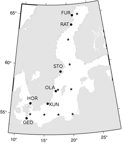
Table 1. Analysed daily tide gauge records

Station name	Lon.(°E)	Lat.(°N)	Missing values (%)
Gedser (GED)	11.93	54.57	4.09
Hornbæk (HOR)	12.47	56.10	3.90
Kungsholmsfort (KUN)	15.58	56.10	0.54
Ölands Norra Udde (OLA)	17.01	57.36	4.01
Stockholm (STO)	18.80	59.31	1.11
Ratan (RAT)	20.92	64.00	0
Furuögrund (FUR)	21.23	64.92	0.22

Tide gauge records of relative sea-level include both sea-level change and vertical land movement signals. The Baltic area experiences significant land uplift associated with GIA (e.g. Ekman and Mäkinen, 1996). Since the focus of the present study is on extreme levels rather than changes in the mean, as a pre-processing step all tide gauge records are linearly detrended, which removes both GIA signals (assuming the influence of isostasy approximately linear) and linear trends in mean sea-level. Furthermore, seasonality (an annual cycle with minimum in spring, cf. Hünicke and Zorita, 2008) is removed by phase averaging (Donner et al., 2008). Missing values (less than 5% for all records, see Table 1) are retained for the quantile regression analysis since it can be performed without interpolation of missing observations. However, gaps in annual block maxima series are linearly interpolated (see Section 4.1).

Daily atmospheric data including air temperature (air T), sea level pressure (SLP) and zonal (u-wind) and meridional (v-wind) wind components are obtained from the NCEP reanalysis (Kalnay et al., 1996). Time series of the atmospheric variables are extracted for the Baltic area (see Fig. 1) from January 1948 to December 2005. A similar pre-processing procedure of linear detrending and deseasoning as used for the tide gauge data is also applied to the reanalysis time series.

3. Statistical methods

3.1. Extreme value theory

Classical extreme value theory allows us to study the asymptotic behaviour of M _n (X):=max(X ₁,…,X _n ), i.e. the maximum order statistic of a sequence of independent and identically distributed random variables X ₁,…,X _n . The limit distribution of M _n (X), properly normalised, can be represented in a single parametric form, the generalised extreme value (GEV) distribution (Katz et al., 2005), given by1

for all x such that 1+ξ(x–µ)/σ>0, with location , scale σ>0 and some shape parameter (also called tail index) . The GEV distribution has three possible forms depending on ξ, namely the Weibull (ξ<0), Gumbel (ξ=0, read as for all ) and Fréchet (ξ>0) distributions. The Fréchet domain of attraction embraces heavy-tailed distributions with polynomially decaying tails, whereas all distribution functions belonging to the Weibull domain of attraction are light-tailed with finite right endpoint. The case ξ=0 is of particular interest for the great variety of distributions ranging from moderately heavy to light-tailed having finite right endpoint or not. Extreme value analysis is based on the fit of the GEV distribution given in eq. (1) to the series M _n (X) of, for example, annual maximum observations. The identification of the particular case of a Gumbel distribution can be based on the log-likelihood (e.g. Coles, 2001)2

provided that for each i=1,…,n, the case ξ=0 being defined by continuity. From eq. (2), a statistical test can be also performed for model selection. The likelihood ratio test allows us to test the hypothesis that a reduced model with likelihood L ₀ is more adequate than a nested model with additional k parameters and likelihood L ₁. The test is based on the statistic Q:=−21n L ₀/L ₁~.

The GEV distribution in eq. (1) assumes a stationary sequence of maxima. To accommodate features often exhibited by extreme sea-levels such as trends, in this analysis the location parameter µ is allowed to vary in time (here given in years) linearly, that is,3

where the parameter β ₁ corresponds to the rate of change in annual maximum sea-level. The scale and shape parameters are assumed to be constant since a large number of parameters hinder the model estimation and is not easily physically interpretable, particularly in the case of the shape parameter. Furthermore, Scotto et al. (2011) assumed for the same dataset of daily tide gauge records a GEV model with time-varying scale parameter but found the corresponding changes in time insignificant, therefore favouring a simpler, constant-scale, GEV model.

The occurrence of extreme sea-levels can be assessed in terms of return levels and return periods. The return period is defined by the inverse of the exceedance probability p of an event and the associated return level z _p is given by:4

3.2. Quantile regression

Quantile regression was introduced by Koenker and Basset (1978) as a method for estimating models of conditional quantile functions, thereby extending the conditional mean model of ordinary least squares regression. For a given random variable Y, the classical linear regression model y=a+bx+ɛ is based on the conditional mean function E[Y|X=x], i.e. the mean of the response variable Y conditional on the value x of the independent variable X. The model parameters a and b are then estimated by minimising the residuals5

The linear quantile regression model6

for a given quantile , where is the quantile function defined as the inverse of the distribution function , is based on the conditional quantile function verifying . The corresponding model parameters are estimated by minimising the sum of asymmetrically weighted absolute residuals7

where ρ(·) is the tilted absolute value function (Koenker and Hallock, 2001). An overview of the quantile regression method and further details can be found in Koenker (2005).

4. Results

4.1. Sea-level maxima

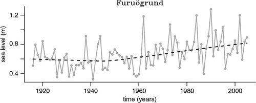
Daily tide gauge records of relative sea-level heights are aggregated in block sizes of one value per year by computing the maximum sea-level for each year. For individual years with more than 60 missing days, the annual maximum is set as missing and replaced by linear interpolation of the adjacent values. This procedure guarantees that the annual maximum is computed from a sample of at least 300 d. This arbitrary 60-d threshold was set after inspection of the records, and the results are not sensitive to its exact value since only a few records have a few, not very large, gaps (see Table 1). It is however important to set such a threshold in order to avoid having non-representative annual maxima computed from only a few days of the year in the case of records with large gaps. The resulting sequence of annual maxima is shown for the Furuögrund station in Fig. 2. Lowess smoothing (Cleveland, 1979) with a smooth span of 2/3 (the proportion of points in the plot which influence the smooth at each value) suggests an apparent increasing trend in annual maxima since the 1950s.

Fig. 2.  Sequence of annual maxima for Furuögrund (solid) and corresponding lowess smooth (dashed).

The extreme value analysis is first performed by fitting the GEV distribution, assuming constant location and scale parameters to the sequence of annual maxima. The value of the estimated shape parameter ξ is assessed from the 95% confidence intervals computed from the corresponding log-likelihood profile (not shown) and indicates for all stations a stationary Gumbel model (ξ=0).

Since a stationary behaviour can be unrealistic for sea-level maxima, particularly in a climate change context, a second model is considered for which µ is represented through the linear expression in eq. (3). The likelihood ratio test is performed to assess the relevance of the shape parameter ξ, i.e. whether a simpler model GEV(µ _t,σ,0) is more adequate than the more complex GEV(µ _t,σ,ξ) model. Similar results as for the stationary case are obtained (see Table 2 and 1 st column). For all stations except Ratan the deviance statistic Q is below the quantile of the theoretical distribution (in this case 3.84) for a 95% confidence level, therefore there is no evidence to reject the null hypothesis of ξ=0. Note that, in the case of Ratan the test statistic is only marginally above the 95% quantile. For Stockholm a non-stationary GEV model with ξ≠0 could not be fitted due to a lack of convergence of the maximum likelihood estimate. In order to assess the relevance of the trend in sea-level maxima, the likelihood ratio test is applied to select between a stationary (i.e. constant µ) and a non-stationary model (Table 2 and 2 nd column). For Kungsholmsfort, Furuögrund and Ratan the null hypothesis of a stationary location parameter is rejected at a 95% confidence level. For Stockholm the test statistic is only slightly below the critical value of the theoretical distribution while for the remaining stations the likelihood ratio test clearly favours the simpler stationary model with constant location parameter.

Table 2. Likelihood ratio test (Q) for the null hypothesis (H ₀) of a Gumbel non-stationary model (ξ=0) and for a stationary model (β ₁=0)

Station name	Q(H 0: ξ=0)	Q(H 0:β 1=0)
Gedser	3.56	0.18
Hornbæk	3.30	0.72
Kungsholmsfort	0.06	5.36
Ölands Norra Udde	2.13	0.03
Stockholm	–	3.49
Ratan	4.12	4.94
Furuögrund	1.46	13.09

For a 95% confidence level, H ₀ is rejected if Q>3.84 (values in bold).

Table 3 summarises the selected models for each station. The adequacy of the estimated models is assessed by diagnostic quantile–quantile plots as illustrated in Fig. 3 for the Furuögrund station.

Fig. 3.  Diagnostics plots: probability plot (left) and quantile-quantile plot (right) for the Furuögrund model.

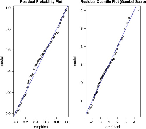
Table 3. Maximum likelihood estimates for µ, σ and ξ of the selected models (standard errors in parentheses)

Station name	µ(mm)	β 0 (mm)	β 1 (mm)	σ (mm)	ξ
Gedser	665.61 (15.66)	140.66 (10.91)	0
Hornbæk	696.69 (16.22)	145.46 (11.43)	0
Kungsholmsfort	428.61 (18.86)	0.87 (0.35)	91.61 (8.17)	0
Ölands Norra Udde	485.07 (13.28)	119.20 (9.55)	0
Stockholm	384.74 (9.87)	89.09 (7.54)	0
Ratan	466.52 (37.38)	1.87 (0.76)	159.61 (13.20)	−154.99 (70.64)
Furuögrund	467.10 (34.32)	2.56 (0.66)	154.42 (12.60)	0

The risk associated with the occurrence of extreme sea-levels can be assessed in terms of return levels for given return periods. Table 4 presents the return values (eq. 4) for 10, 25, 50 and 100 yr. Some considerations of practical order are required at this point for the calculation of the return values of the non-stationary models (Kungsholmsfort, Ratan and Furuögrund). For numerical purposes, it is preferable to re-scale first the year variable so that it is centred. In this case, t*=(year t−starting year)/number of years, with t=2015, 2030, 2055 and 2105, corresponding to p=0.1, 0.04, 0.01 and 0.01 in (eq. 4), was used. Hence, the return values of the non-stationary models are calculated from (eq. 4) with µ=µ(t)=β ₀+β ₁ t*.

Table 4. Return levels (m) for 10, 25, 50 and 100 yr

Return levels (m)
Station	10 yr	25 yr	50 yr	100 yr
Gedser	0.98	1.12	1.21	1.31
Hornbæk	1.02	1.16	1.26	1.37
Kungsholmsfort	0.64	0.73	0.79	0.86
Ölands Norra Udde	0.75	0.87	0.95	1.03
Stockholm	0.56	0.67	0.73	0.79
Ratan	0.77	0.87	0.94	1.00
Furuögrund	0.83	0.98	1.09	1.20

4.2. Quantile trends

Quantile slopes of the linear quantile regression model (eq. 7) are estimated from eq. (8) by numerical optimisation (Koenker and D'Orey, 1987). Figure 4 shows the resulting slopes for quantiles 0.5 (median) to 0.98 since the interest for comparison with the annual maxima results is on the upper quantiles. Table 5 displays the slope values for quantile 0.98 for all tide gauge records. Since uncertainty increases away from the central part of the distribution, standard errors are higher for the more extreme quantiles. The 0.98 quantile is therefore a trade-off between a high-enough quantile and a still reasonably low uncertainty. As an alternative approach to assess uncertainty, a bootstrap procedure that preserves the temporal dependence of the data (Vinod and Lopez-de-Lacalle, 2009) is applied as in Barbosa et al. (2011). Estimates of the quantile slope are described by the median of the ensemble and the associated uncertainty by the ensemble interquartile range (IQR). Since the bootstrap uncertainty is lower (Table 5 and 2 nd column), the maximum likelihood uncertainty is used henceforth. Table 5 indicates a clear latitudinal dependence with larger sea-level trends for the northernmost stations. Barbosa (2008) and Donner et al. (2012) found statistically significant differences between the 0.90 and the median quantile slopes for the Stockholm and Ratan stations, which are consistent with the results of the present study. However, in these studies monthly rather than daily data were examined, the pre-processing of the records was distinct and a different set of tide gauge records was considered. This explains the quantitative disagreement with the quantile regression results of the present study.

Fig. 4.  (Continued)

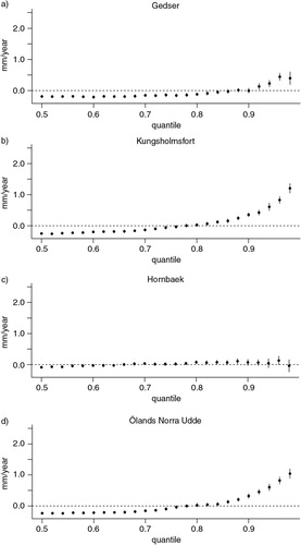
Fig. 4.  Quantile slopes (points) and corresponding standard errors (vertical error bars). The horizontal dashed line denotes the mean (0 mm/yr) trend.

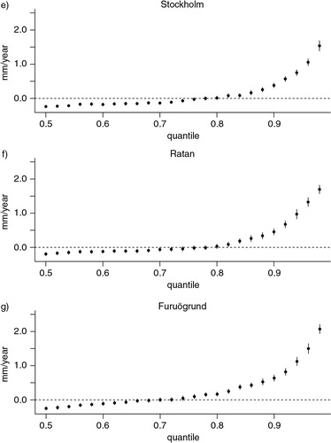
Table 5. Quantile regression trends (standard errors in parentheses) and corresponding bootstrap estimates (ensemble median and IQR) for quantile 0.98

Station	Slope (mm/yr)	Ensemble median (mm/yr)
Gedser	0.40* (0.22)	0.40 (0.05)
Hornbæk	−0.04 (0.18)	−0.04 (0.02)
Kungsholmsfort	1.20* (0.14)	1.23 (0.06)
Ölands NorraUdde	1.04* (0.13)	1.05 (0.07)
Stockholm	1.54* (0.15)	1.55 (0.07)
Ratan	1.70* (0.12)	1.74 (0.08)
Furuögrund	2.07* (0.14)	2.10 (0.08)

Statistically significant trends (95% confidence level) are denoted by *.

4.3. Atmospheric extremes

A similar extreme value analysis is performed for the atmospheric time series from the NCEP reanalysis dataset. Table 6 displays the results of the likelihood ratio test for a stationary (β ₁=0) versus non-stationary (β ₁≠0) GEV model for the annual maxima series of atmospheric variables. For SLP, the maxima are stationary at all locations. A stationary model is also favoured for all the atmospheric variables at the two gridpoints closest to the Baltic entrance (12.5°E, 55°N; 15°E, 55°N) and in the Bothnian Sea (20°E, 60°N; 20°E, 62.5°N). For the non-stationary GEV models, the corresponding slopes of the annual maxima are shown in Table 7. Air temperature maxima exhibit an increasing trend for the series in the Baltic Proper. Both zonal and meridional winds display an increasing trend in the Western Baltic and at the northernmost reanalysis gridpoint in the Bothnian Bay. Furthermore, a positive slope is found in the Central Baltic for meridional wind maxima.

Table 6. Likelihood ratio test (Q) for the null hypothesis (H ₀) of a stationary GEV model (β ₁=0) for the atmospheric data

Gridpoint	Air T	SLP	u-wind	v-wind
12.5°E 55.0°N	3.13	0.82	2.01	0.68
15.0°E 55.0°N	2.59	0.96	–	–
17.5°E 55.0°N	4.20	1.22	20.54	12.65
20.0°E 55.0°N	2.33	1.49	16.33	11.87
17.5°E 57.5°N	4.92	0.83	0.17	2.8
20.0°E 57.5°N	2.27	1.08	0	5.76
20.0°E 60.0°N	1.74	0.30	0.07	0.16
20.0°E 62.5°N	1.78	0.44	1.61	0.29
22.5°E 65.0°N	0.83	0.98	15.75	5.70

For a 95% confidence level, H ₀ is rejected if Q>3.84 (values in bold)

Table 7. Maximum likelihood estimates for the slope (β ₁) of the non-stationary GEV models (standard errors in parentheses)

Air T	u-wind	v-wind
Gridpoint	(°C/decade)	(10^−3 ms ^−1/yr)	(10^−3 ms ^−1/yr)
12.5°E 55.0°N	–	–	–
15.0°E 55.0°N	–	–	–
17.5°E 55.0°N	0.28 (0.13)	0.62 (0.0020)	0.31 (0.0021)
20.0°E 55.0°N	–	0.54 (0.0020)	0.32 (0.0036)
17.5°E 57.5°N	0.22 (0.10)	–	–
20.0°E 57.5°N	–	–	0.31 (0.0020)
20.0°E 60.0°N	–	–	–
20.0°E 62.5°N	–	–	–
22.5°E 65.0°N	–	0.30 (0.0020)	0.21 (0.0045)

Quantile regression results for the atmospheric reanalysis variables are displayed in Table 8 for quantile 0.98. Air temperature exhibits an increasing trend at all the considered locations. In the case of atmospheric pressure, a positive slope is found for the gridpoints below 60°N. Zonal winds increase at all locations except the two gridpoints in the Central Baltic Proper while meridional winds increase in the Western Baltic and also in the northernmost point in the Bothnian Bay.

Table 8. Quantile regression trends (standard errors in parentheses) for quantile 0.98

Air T	SLP	u-wind	v-wind
Gridpoint	(°C/decade)	mbar/yr	(10^−3 ms ^−1/yr)	(10^−3 ms ^−1/yr)
12.5°E 55.0°N	0.17 (0.039)*	0.035 (0.012)*	0.28 (0.054)*	0.076 (0.046)
15.0°E 55.0°N	0.14 (0.041)*	0.042 (0.012)*	0.42 (0.054)*	0.081 (0.040)*
17.5°E 55.0°N	0.16 (0.041)*	0.039 (0.011)*	0.42 (0.059)*	0.20 (0.038)*
20.0°E 55.0°N	0.16 (0.040)*	0.048 (0.011)*	0.33 (0.055)*	0.21 (0.037)*
17.5°E 57.5°N	0.20 (0.036)*	0.034 (0.012)*	0.030 (0.058)	−0.028 (0.050)
20.0°E 57.5°N	0.19 (0.035)*	0.030 (0.013)*	0.023 (0.063)	−0.076 (0.052)
20.0°E 60.0°N	0.19 (0.031)*	0.0067 (0.013)	0.11 (0.051)*	−0.0002 (0.051)
20.0°E 62.5°N	0.078 (0.037)*	−0.011 (0.013)	0.093 (0.045)*	0.032 (0.043)
22.5°E 65.0°N	0.12 (0.028)*	−0.025 (0.016)	0.18 (0.051)*	0.083 (0.04)*

Statistically significant trends (95% confidence level) are denoted by *.

5. Discussion and conclusions

A GEV approach was applied for the analysis of extreme events in the Baltic Sea, assuming both constant and time-varying parameters. Arguably, the sea-level annual maxima is well fitted through a Gumbel distribution, in agreement with results obtained for other tide gauge stations in the Baltic, specifically at the Estonian coast (Suursaar and Sooaar, 2007).

The results show a clear latitudinal dependence, with the northernmost stations (Furuögrund, Ratan) exhibiting a statistically significant trend in annual sea-level maxima while for the remaining stations extremes can be adequately represented by a stationary Gumbel model. The estimated non-stationary model indicates that sea-level maxima are increasing relative to the mean at a rate of 1.87 (±0.76) mm/yr and 2.56 (±0.66) mm/yr at Ratan and Furuögrund, respectively. Note that these trends in maxima were derived from detrended time series, i.e. with no trend in the mean. For the other tide gauges, the maxima can be considered stationary over the analysed period, and the highest return levels are obtained for the stations at the Baltic entrance, Gedser and Hornbæk.

The derived quantile regression slopes are consistent with the extreme value theory results, with also a clear latitudinal effect and higher slopes for the stations further north. The smallest quantile slopes are obtained for the stations in the Baltic entrance, in agreement with the non-significant slopes obtained with a non-stationary GEV distribution. For the tide gauges at intermediate latitudes, the annual maxima are stationary while the corresponding slopes for the 98% quantile are statistically significant but relatively small (1−1.5 mm/yr). For the northern stations, the quantile slopes are slightly lower than the computed trends in annual sea-level maxima from the extreme value model. Quantitative differences between (non-stationary) extreme value and quantile regression analysis are not surprising since beyond the methodological differences of the two approaches trends in the 98% quantile and in annual maxima are not expected to be exactly the same.

The largest return levels are found for the stations at the ends of the Baltic: the Danish stations (Gedser, Hornbæk) and the stations in the Gulf of Bothnia (Ratan, Furuögrund) which are more affected by storm events than the stations in the central part of the Baltic (e.g. Andersson, 2002; Ekman, 2007). At the Baltic entrance, both sea-level and atmospheric variables are characterised by stationary distributions. In contrast, the northernmost stations exhibit a non-stationary behaviour in the form of a significant trend in the annual maxima, suggesting that additional processes other than storms are responsible for the observed behaviour of sea-level extremes. Return levels and trends are lower in the Central Baltic area despite being the region with higher trends in air temperature, which is consistent with a stronger influence of winds rather than temperature on sea-level changes. Persistent winds have a strong influence in the variability of Baltic Sea-level (e.g. Samuelsson and Stigebrandt, 1996), and large-scale processes such as the NAO (e.g. Lehmann et al., 2002; Hünicke and Zorita, 2006; Bastos et al., 2013) affect the wind patterns over the Baltic area. The reanalysis results show significant positive trends in both meridional and zonal winds over the Western Baltic and also at the end of the Baltic in the Bothnian Bay. Despite the different period covered by the tide gauge and the reanalysis data, such changes in wind speed identified over the 20th century are a likely candidate for explaining the increase in sea-level maxima in the northern Baltic.

6. Acknowledgements

This work was done in the framework of the PEST-OE/CTE/LA0019/2013-2014 program, financed by FCT.

References

- Andersson H . Influence of long-term regional and large-scale atmospheric circulation on the Baltic Sea level. Tellus A. 2002; 54: 76–88.
- Barbosa S . Quantile trends in Baltic Sea level. Geophys. Res. Lett. 2008; 35: L22704.
- Barbosa S. M. , Madsen K. S . Kenyon S. , Pacino M. C. , Marti U . Quantile analysis of relative sea-level at the Hornbæk and Gedser Tide Gauges. Geodesy for Planet Earth: Proceedings of the 2009 IAG Symposium. 2012; Berlin Heidelberg: Springer. 567–571.
- Barbosa S. M. , Scotto M. G. , Alonso A. M . Summarising changes in air temperature over Central Europe by quantile regression and clustering. Nat. Hazard Earth Syst. 2011; 11: 3227–3233.
- Bastos A. , Trigo R. , Barbosa S. M . Discrete wavelet analysis of the influence of the North Atlantic Oscillation on Baltic Sea level. Tellus A. 2013; 65: 20077.
- Cleveland W. S . Robust locally weighted regression and smoothing scatterplots. J. Am. Stat. Assoc. 1979; 74: 829–836.
- Coles S . An Introduction to Statistical Modeling of Extreme Values. 2001; Springer-Verlag, London.
- Dangendorf S. , Mudersbach C. , Jensen J. , Ganske A. , Hartmut H . Seasonal to decadal forcing of high water level percentiles in the German Bight throughout the last century. Ocean Dynam. 2013; 63: 533–548.
- Donner R. , Sakamoto T. , Tanizuka N . Donner R. V. , Barbosa S. M . Complexity of spatio-temporal correlations in Japanese air temperature records. Nonlinear Time Series Analysis in the Geosciences – Applications in Climatology, Geodynamics, and Solar-Terrestrial Physics. 2008; Berlin: Springer. 125–154.
- Donner R. V. , Ehrcke R. , Barbosa S. M. , Wagner J. , Donges J. F. , co-authors . Spatial patterns of linear and nonparametric long-term trends in Baltic sea-level variability. Nonlinear Process Geophys. 2012; 19: 95–111.
- Ekman M . Climate changes detected through the world's longest sea level series. Glob. Planet. Change. 1999; 21: 215–224.
- Ekman M . A Secular Change in Storm Activity over the Baltic Sea Detected through Analysis of Sea Level Data. 2007; Åland Islands: Small Publications in Historical Geophysics 16. Summer Institute for Historical Geophysics.
- Ekman M . The Changing Level of the Baltic Sea During 300 Years: A Clue to Understanding the Earth. 2009; Åland Islands: Summer Institute for Historical Geophysics.
- Ekman M. , Mäkinen J . Recent postglacial rebound, gravity change and mantle flow in Fennoscandia. Geophys. J. Int. 1996; 126: 229–234.
- Gräwe U. , Burchard H . Storm surges in the Western Baltic Sea: the present and a possible future. Clim. Dynam. 2012; 39: 165–183.
- Hansen L . Hourly values of sea level observations from two stations in Denmark Hornbæk 1890–2005 and Gedser 1891–2005. DMI Technical Report. 2007; Copenhagen: Danish Meteorological Institute. No 07-09.
- Hünicke B. , Zorita E . Influence of temperature and precipitation on decadal Baltic Sea level variations in the 20th century. Tellus A. 2006; 58: 141–153.
- Hünicke B. , Zorita E . Trends in the amplitude of Baltic Sea level annual cycle. Tellus A. 2008; 60: 154–164.
- Jevrejeva S. , Moore J. , Woodworth P. , Grinsted A . Influence of large-scale atmospheric circulation on European sea level: results based on the wavelet transform method. Tellus A. 2005; 57: 183–193.
- Johansson M. , Boman H. , Kahma K. , Launiainen J . Trends in sea level variability in the Baltic Sea. Boreal Environ. Res. 2001; 6: 159–179.
- Kalnay E. , Kanamitsu M. , Kistler R. , Collins W. , Deaven D. , co-authors . The NCEP/NCAR 40-year reanalysis project. Bull. Am. Meteorol. Soc. 1996; 77: 437–470.
- Katz R. W. , Brush G. S. , Parlange M. B . Statistics of extremes: modelling ecological disturbances. Ecology. 2005; 86: 1124–1134.
- Koenker R . Quantile Regression. 2005; Cambridge University Press, New York.
- Koenker R. , Basset G . Regression quantiles. Econometrica. 1978; 46: 33–50.
- Koenker R. , D'Orey V . Computing regression quantiles. Appl. Stat. 1987; 36: 383–393.
- Koenker R. , Hallock K . Quantile regression. J. Econ. Perspect. 2001; 15: 143–156.
- Lehmann A. , Krauss W. , Hinrichsen H.-H . Effects of remote and local atmospheric forcing on circulation and upwelling in the Baltic Sea Journal. Tellus A. 2002; 54: 299–316.
- Menéndez M. , Woodworth P. L . Changes in extreme high water levels based on a quasi-global tide-gauge data set. J. Geophys. Res. 2010; 115: 10011.
- Mudersbach C. , Jensen J . Nonstationary extreme value analysis of annual maximum water levels for designing coastal structures on the German North Sea coastline. J. Flood Risk Manage. 2010; 3: 52–62.
- Samuelsson M. , Stigebrandt A . Main characteristics of the long-term sea level variability in the Baltic sea. Telllus A. 1996; 48: 672–683.
- Scotto M. G. , Barbosa S. M. , Alonso A. M . Wright L. L . Model-Based Clustering of Extreme Sea Level Heights. Sea Level Rise, Coastal Engineering, Shorelines and Tides. 2011; New York: Nova Science Publishers. 277–293. Chapter 15.
- Suursaar U. , Kullas T. , Otsmann M. , Kuts T . Extreme sea level events in the coastal waters of western Estonia. J. Sea Res. 2003; 49: 295–303.
- Suursaar U. , Sooaar J . Decadal variations in mean and extreme sea level values along the Estonian coast of the Baltic Sea. Tellus A. 2007; 59: 249–260.
- Vinod H. D. , Lopez-de-Lacalle J . Maximum entropy bootstrap for time series: the meboot r package. J. Stat. Software. 2009; 29: 1–19.