Seasonal-to-decadal predictions with the ensemble Kalman filter and the Norwegian Earth System Model: a twin experiment

Abstract

Here, we firstly demonstrate the potential of an advanced flow dependent data assimilation method for performing seasonal-to-decadal prediction and secondly, reassess the use of sea surface temperature (SST) for initialisation of these forecasts. We use the Norwegian Climate Prediction Model (NorCPM), which is based on the Norwegian Earth System Model (NorESM) and uses the deterministic ensemble Kalman filter to assimilate observations. NorESM is a fully coupled system based on the Community Earth System Model version 1, which includes an ocean, an atmosphere, a sea ice and a land model. A numerically efficient coarse resolution version of NorESM is used. We employ a twin experiment methodology to provide an upper estimate of predictability in our model framework (i.e. without considering model bias) of NorCPM that assimilates synthetic monthly SST data (EnKF-SST). The accuracy of EnKF-SST is compared to an unconstrained ensemble run (FREE) and ensemble predictions made with near perfect (i.e. microscopic SST perturbation) initial conditions (PERFECT). We perform 10 cycles, each consisting of a 10-yr assimilation phase, followed by a 10-yr prediction. The results indicate that EnKF-SST improves sea level, ice concentration, 2 m atmospheric temperature, precipitation and 3-D hydrography compared to FREE. Improvements for the hydrography are largest near the surface and are retained for longer periods at depth. Benefits in salinity are retained for longer periods compared to temperature. Near-surface improvements are largest in the tropics, while improvements at intermediate depths are found in regions of large-scale currents, regions of deep convection, and at the Mediterranean Sea outflow. However, the benefits are often small compared to PERFECT, in particular, at depth suggesting that more observations should be assimilated in addition to SST. The EnKF-SST system is also tested for standard ocean circulation indices and demonstrates decadal predictability for Atlantic overturning and sub-polar gyre circulations, and heat content in the Nordic Seas. The system beats persistence forecast and shows skill for heat content in the Nordic Seas that is close to PERFECT.

• seasonal-to-decadal prediction
• EnKF
• NorESM
• NorCPM
• SST initialisation

1. Introduction

The 5^th assessment of the International Panel on Climate Change (IPCC), scheduled for 2014, will partly be dedicated to evaluate the feasibility of decadal-scale climate predictions (Taylor et al., 2012). Skilful predictions on inter-annual to decadal timescales will fill the gaps between the established fields of seasonal forecasting and future climate change projections (Meehl et al., 2009). Up to decadal time scales, climate prediction is crucially dependent on the accuracy of the initial conditions (Hawkins and Sutton, 2009; Branstator and Teng, 2010; Branstator et al., 2012). Because the thermal inertia of the ocean is much larger than that of the atmosphere or land, one may assume that the ocean has a key role in the predictability of the climate system on these timescales. The initialising of seasonal predictions has advanced significantly over the last 20 yr. The application of these methods to seasonal-to-decadal prediction is only just being investigated.

Different classes of methodologies have been used for model initialisation in seasonal-to-decadal predictions. Smith et al. (2008), Pohlmann et al. (2009) and Tatebe et al. (2012) use restoring (nudging) on 3-D ocean reanalysis products, restoring only the anomalies to limit the impact from model bias. This class of methodology shows some skill, in particular in the North Atlantic, but has several drawbacks. First, it relies on the time coverage of existing reanalysis; second, this two-step approach amplifies the problem of model biases for data assimilation because observations are filtered twice and the bias in the reanalysis differs from the bias in the forecast system.

A second class of methodology uses the same model for data synthesis and forecasts. Pohlmann et al. (2009) anticipated that this approach will lead to the best forecast results. Restoring of model sea surface temperature (SST) to observation were used in coupled simulations; this technique shows skill in predicting SST on seasonal and decadal timescales in the tropical Pacific and on decadal timescales in the North Atlantic, despite strong drift in the Atlantic Meridional Overturning Circulation (AMOC) (Keenlyside et al., 2005, 2008; Luo et al., 2005). Using the same technique, Dunstone et al. (2011) show that relaxation towards SST is not sufficient to constrain the AMOC and the Subpolar Gyre (SPG) variations, whereas this is ameliorated by including additional Argo float observations. Swingedouw et al. (2012) use a weaker relaxation than the previous studies and demonstrate predictability for AMOC and SPG with up to a 4-yr lead-time. Zhang et al. (2007, 2009 2010) investigate the capability of a more advanced data assimilation method based on the ensemble Kalman filter (EnKF). Zhang et al. (2007) show that the combined updates of temperature and salinity avoid the introduction of model drift. Zhang et al. (2009, 2010) test the predictability of their system in twin experiments and investigate the benefit of different observation networks. They suggest that combined assimilation of SST and atmospheric data can control variability of AMOC during the analysis period, and that addition of Argo floats data are beneficial for controlling variability in the North Atlantic. However, their implementation considers only an update of the surface (vertical scale of 10 m for SST), despite the fact that ensemble data assimilation methods can also be beneficial in deeper water (Haugen and Evensen, 2002; Brusdal et al., 2003; Counillon and Bertino, 2009). Furthermore, updating the entire water column may provide a more consistent update (Srinivasan et al., 2011).

This study has two aims: (1) to reassess the use of SST data for seasonal-to-decadal prediction using a more advanced scheme compared to previous studies; (2) to demonstrate the potential use of the advanced EnKF data assimilation with a full ocean state update for such predictions. The other components of the earth system model are not updated by assimilation. The study utilises twin experiments and does not address the issue of model bias (i.e. assumes a perfect model). Pseudo SST observations are extracted from a control run with identical model configuration and constant external forcing consistent with pre-industrial conditions (i.e. without temporal reference). The primary advantage of such a framework is that an extensive validation is possible, as the full state is known. A second advantage is that the system can be tested in a non-biased configuration. Model biases are problematic for data assimilation (Dee, 2005) and dedicated investigations are necessary before assimilating real observations. Here we only assimilate SST, as one of our objectives is to assess the potential of performing hindcasts over the relatively long period that SST have been routinely measured (i.e. from around 1870). The current hindcast period for decadal predictions is rather limited, beginning around the 1960s when hydrographic data became more plentiful. Our study extends over a 100-yr window in order to sample ascending, descending and transient phases of the SPG and AMOC. Anthropogenic (greenhouse gases and aerosols) and natural forcing (volcanic and solar) can influence the multi-decadal variability in the Atlantic (Otterå et al., 2010; Swingedouw et al., 2012), but they are not considered here because we wish to focus on the potential predictability associated with ocean variability. This differs from the CMIP5 experiment design (Taylor et al., 2012) for which predictability is tested between 1960 and 2005 using external forcing and initialisation from real observations.

A special emphasis for Norwegian Climate Prediction Model (NorCPM) is placed in the Nordic Seas and the Arctic. Climate variability in the Nordic Seas is of interest for several reasons. Changes in dense water formation are communicated via the overflows to the North Atlantic, where they modulate the strength of the large-scale ocean overturning circulation (e.g. Schweckendiek and Willebrand, 2005). Heat transport variability affects the position of the sea ice edge (e.g. Bengtsson et al., 2004; Bitz et al., 2005), which is potentially important for extreme winter events over Europe (Petoukhov and Semenov, 2010). Ocean temperature changes also have direct consequences for the fish stocks and ecosystem variability in this region (Loeng and Drinkwater, 2007). However, the question of how well the internal climate variability can be predicted in the Nordic Seas remains open. Hydrographic section data show persistent surface temperature anomalies that seemingly propagate along the path of the Atlantic Water to the Arctic and thus may give rise to regional climate predictability at sub-decadal time scales (Holliday et al., 2008). Other studies suggest that exchange processes between the Atlantic and Arctic Oceans drive multi-decadal climate variability on 50–70 yr time scales (Jungclaus et al., 2005; Frankcombe et al., 2010). Finally, in the North Atlantic, the amplitude of the decadal variability is comparable to the inter-annual variability (Boer, 2004; Latif et al., 2006), which is mainly driven by the atmospheric response and is poorly predictable. Consequently, skill in decadal prediction – assuming it can be achieved – would have a substantial overall impact with respect to the poorly predictable part.

The outline of the paper is as follows. The model system is presented in Section 2, the data assimilation method in Section 3 and the experimental set-up in Section 4. In Section 5, the model is studied in analysis mode – while observations of SST are assimilated. It includes a quantitative comparison followed by a comparison against standard ocean circulation indices. In Section 6, a similar comparison is performed in prediction mode. The prediction system is compared to the trivial persistence forecast and to the upper ‘perfect’ prediction limit. Finally, the skill of NorCPM is assessed with respect to our primary area of interest, the Nordic Seas.

2. Model system: Norwegian Earth System Model

The Norwegian Earth System Model (NorESM; Bentsen et al., 2013) is based on the Community Earth System Model version 1.0.3 (CESM1; Vertenstein et al., 2012), which is the successor of the Community Climate System Model version 4 (CCSM4; Gent et al., 2011). The ocean component is replaced with an updated version of the Miami Isopycnic Coordinate Model (MICOM; Bleck et al., 1992). Major updates to MICOM include the implementation of incremental remapping for isopycnal advection, estimation of the pressure gradient force through accurate vertical integration of in-situ density, modified parameterisation of isopycnal and diapycnal mixing processes, and a new split-mixed layer formulation (Bentsen et al., 2013). NorESM has options for a comprehensive treatment of aerosol and cloud chemistry (Kirkevåg et al., 2012), as well as ocean biogeochemistry (Assmann et al., 2010; Tjiputra et al., 2012); these are, however, deactivated in this study. Otherwise, the atmosphere (CAM4), land (CLM4), sea ice (CICE4) and coupler (CPL7) components are the same as in CESM1.

This study uses the low-resolution NorESM1-L (Zhang et al., 2012) set-up, which has the same grid configuration as the low-resolution CCSM4 (Shields et al., 2012). The atmospheric component is configured with a spectral horizontal truncation of T31, corresponding to a nominal resolution of 3.75°, and 26 hybrid pressure levels in the vertical, ranging from the surface to 3 hPa. The ocean component uses the standard grid gx3v7 [version 7 of the Greenland pole with a horizontal resolution of approximately 3° (x3)] provided by CCSM4, which has a longitudinal resolution of 3.6° at the Equator. The Northern Hemisphere grid singularity is placed over Greenland and the Southern Hemisphere grid singularity is located at the geographical south pole. In the vertical, the ocean component comprises a stack of 30 isopycnic layers with a two-layer bulk mixed layer on top. The potential density of the layers, referenced to 2000 dbar, ranges from 1027.6 to 1037.4 kg m⁻³, and differs from the ones adopted for past climate simulations in Zhang et al. (2012).

The external forcings are fixed to the pre-industrial level of 1850. The simulated global mean temperature at 2 m of 11.8°C is approximately 2°C colder compared to modern estimates (see e.g. Jones et al., 1999). This cold bias is associated with an exaggerated sea ice cover with seasonal minimum and maximum sea ice extents of 10.3×10⁶ km² and 17×10⁶ km² in the Northern Hemisphere, and 5.5×10⁶ km² and 18.6×10⁶ km² in the Southern Hemisphere. Corresponding satellite estimates of sea ice extent are 8.5×10⁶ km² and 15×10⁶ km² (Parkinson and Cavalieri, 1989) and 4×10⁶ km² and 17×10⁶ km² (Zwally et al., 2002) for the Northern and Southern Hemispheres, respectively. The system is able to reproduce well the seasonal variability of SST along the Equator. However, variability of the simulated El Niño Southern Oscillation (ENSO) is somewhat too weak and exhibits a dominant period of approximately 2 yr instead of 4–6 yr as seen in observations (Philander, 1990; Wittenberg, 2009). The simulated mean strength of the AMOC is 16.4 Sv at 24°N (18.0 Sv at 42°N and 21.2 Sv within the latitudinal band 20–60°N) and compares well with observational estimates of 13–24 Sv (Medhaug and Furevik, 2011, and references within). The simulated mean strength of the North Atlantic SPG is 54 Sv, which is somewhat higher than observational estimates of 35–50 Sv (Han and Tang, 2001).

3. Ensemble Kalman Filter

The EnKF is a sequential data assimilation method that consists of two steps, a propagation and a correction. The propagation step is a Monte Carlo method. An ensemble of N model states (X) is integrated forward in time. The ensemble of states is denoted by:1

where n is the size of the model state. The ensemble spread (i.e. ensemble variability) is used to estimate the forecast error, because we expect them to be related in locations (and times) where (and when) the system is more chaotic. Furthermore, assuming that the distribution of the error is Gaussian and the model is not biased, the ensemble mean () provides the best estimator and the model covariance (C) may be used to quantify the forecast error (ε):2

where the superscript ^T denotes a matrix transpose and X′ the ensemble anomaly (i.e. , where is of size N×1 with all elements equal to 1). During the correction step, the method uses the observations (Y) and their covariance matrix (R) to estimate a new ensemble of model states. The observation error covariance matrix R is diagonal in our case. The solution minimises the variance of the deviation from an unknown ‘truth’. Here, we use the Deterministic EnKF (Sakov and Oke, 2008), which is a square-root version of the EnKF. The algorithm solves the analysis/correction step in two sub-steps: the first sub-step is the estimation of the ensemble mean that minimises the distance from the truth based on its distance from observations while in the second sub-step, the ensemble anomaly is updated to adjust the covariance. The first sub-step is written as:3

where the superscript ‘a’ refers to the analysis state and ‘f’ to the forecast, and H is the measurement operator relating the prognostic model state variables to the measurements. The Kalman Gain (K) is computed as follow:4

Finally, the second sub-step, is written as:5

The method allows for 3-D and multivariate model updates using the model ensemble covariance matrix. Evensen (2003) demonstrated that the EnKF conserves the linear properties of the state variables. When the full model state is updated throughout the water column, this implies that the method conserves geostrophy and ensures that the sum of all layer thicknesses is consistent with the bottom pressure. This remains valid when using the Deterministic EnKF (DEnKF). A distance-based localisation method is used - known as ‘local analysis’ (Evensen, 2003). As the horizontal resolution of the ocean model is larger than the expected decorrelation radius in some regions (approximately 50–200 km in the North Atlantic, Krauss et al., 1990), the impact of observations is limited to the water column properties. The spatial smoothness of the update is ensured by autocorrelation in the observations, which are provided at every grid cell (except below the sea ice). It is reasonable to assume that an ensemble of 30 members is sufficiently large to represent the model subspace of a water column. Nevertheless, the limited ensemble size and unfulfilled prior assumptions make the system suboptimal, which leads to an excessive reduction of the ensemble spread. Here, instead of using the classical ensemble inflation (Anderson, 2001), moderation is used. This consists of increasing observation error (here by a factor 2) for the update of the error covariance [eq. (5)] while the original error variance is kept for the update of the ensemble mean in eq. (3) (Sakov et al., 2012). Another technique referred to as pre-screening of the observation is employed in location where model and observations happen to be too far apart. When the innovation is too large compared to the forecast error, assimilation of this observation is likely to produce an unbalanced analysis. The impact of the observation is artificially reduced (observation error increased) as proposed in Sakov et al. (2012). Note that we have not included model error because our experiment is an identical twin experiment and our model is thus perfect.

A monthly assimilation cycle is used in this study. The ensemble forecast, X ^f consists of the ensemble of restart files in the middle of the month and monthly averaged observations are assimilated. Analysis is only applied to the first time level (of the leap frog scheme) and copied to the second time level, although some benefit may be obtained by assimilating both time levels (Zhang et al., 2004). The initial ensemble is composed from the output of the control run (see Section 4). The motivation for using this approach is to ensure that a sufficient ensemble spread is found in the interior of the ocean. In order to limit the impact from an abrupt start of data assimilation, the observation error variance is inflated by a factor of 8 and gradually decreased over five assimilation cycles (5 months).

Application of the EnKF to an isopycnal coordinate model has some challenges:

• When both potential temperature (only temperature is used hereafter) and salinity are updated, the analysis consists of the combination of the initial ensemble within a given isopycnal coordinate. Combining water masses with the same density introduces artificial caballing. The updated analysis field will have denser water than before the update. If the resulting density is far from the reference density, instabilities are introduced in the model stratification enhancing spurious mixing (Counillon and Bertino, 2009). However, Srinivasan et al. (2011) demonstrated that as the density gradients are often small, the benefits of updating both temperature and salinity are larger than that of updating only one (e.g. temperature) and diagnosing the other from the reference density.

• The EnKF assumes that the distribution of the error is Gaussian, which is not always the case. In particular, layer thickness has a truncated Gaussian distribution. The variables updated by the analysis are ‘gaussianised’, which may produce negative layer thickness values. Such values are corrected here in a post-processing step, where the missing volume is taken from the first non-negative layer below. A more elegant solution to this problem is to use a Gaussian anamorphosis method (Bertino et al., 2003; Simon and Bertino, 2009) or to solve the analysis with additional constraints (Thacker, 2007).

• In MICOM that uses the hydrostatic approximation and isopycnic vertical coordinate, isopycnic model layers become massless, or empty, when the layer's reference potential density falls outside the range of potential densities present in the water column. With a bulk surface mixed layer with varying potential density, these empty layers can be present at the ocean floor or at the base of the mixed layer. In empty layers, the temperature is extrapolated from neighbouring non-empty layers and salinity is computed to satisfy the reference potential density. For a specific 3-D location, an ensemble may contain a combination of empty and non-empty layers and due to the unphysical construction of layer properties of empty layers, this leads to a problem when computing the covariance. Particularly at the base of the mixed layer the unphysical values in empty layers have been found to corrupt the covariance and—if not corrected—introduce a drift in the model water properties below the mixed layer depth. In order to circumvent this problem, the value of the water masses in the empty layers is replaced by the average of the non-empty layers in the other ensemble members. As such, the water properties in empty layers become ‘neutral’ in the EnKF algorithm. This ad-hoc solution ensures that the ensemble mean is conserved, but the value of the ensemble variance is underestimated. This solution proves successful in most places, and no severe drift appears in the accuracy of the system. Nevertheless, a weak drift for salinity and temperature is found at intermediate depth (colder and fresher), when assimilating for periods longer than 10 yr. This drift originates from weakly stratified regions with large inter-annual variability (e.g. near Antarctica). There, opening a layer and filling it with an ensemble average is not necessarily consistent with the rest of the vertical water column that receives corrections computed from their distance to the ensemble mean. This introduces an instability, which is dampened in MICOM by convection, enhancing mixing with the colder and fresher water from the mixed layer depth. However, this is not considered problematic for this study because the analysis window is set to 10 yr and the initial ensemble is re-initialised for each prediction cycle. Other alternatives are considered in the discussion for performing longer simulation.

4. Experimental set-up

This study uses a twin-experiment framework and the experimental set-up is described in Fig. 1. The ‘truth’ solution (henceforth referred to as TRUTH) is the year 601–710 of a multi-century control run. The model has very little drift so that the framework can be considered as bias free. Nevertheless, some drift exists in the system, as for example in mean sea level with an increase of 2 cm/100 yr.

Fig. 1 Schematic of the experimental set-up. TRUTH (in grey) is the year 600–710 of a multi-century control run. PERFECT (in red) is initialized from TRUTH at the beginning of each prediction cycle. The 10 EnKF-SST cycles assimilate observations extracted from TRUTH during the analysis period and continued in the prediction cycles. The analysis cycle of EnKF-SST (in blue) and FREE (in black) are initialised from the same initial ensemble (green ellipse) composed from output of the years 251–541 of the control run.

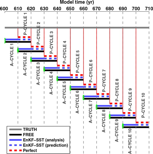
Observations are extracted from monthly averages of TRUTH with a random white noise (std =0.1°C) added to simulate observational error. Note that using a white noise for observation error implies that we are neglecting the problems of observational bias and spatially correlated observation error that would have degraded the performance of our prediction. Data in ice-covered water is discarded, consistent with the coverage of real observations.

The EnKF experiment assimilates synthetic SST and is henceforth referred to as EnKF-SST. There are 10 cycles of 20 yr, which consist of a 10-yr analysis period followed by a 10-yr prediction period. Each cycle is initialised from the identical initial ensemble that is composed from the control run during the year 251–541 with a frequency of 10 yr. As the same initial ensemble is used for initialising each analysis cycle, each cycle is equally likely and it is possible to compute the averaged accuracy (or the correlation) at a given time of the cycle.

This system is compared to a free ensemble that is henceforth referred to as FREE. The same 30 initial conditions (restart files) are used in EnKF-SST and FREE so that a direct comparison is possible. As EnKF-SST is reinitialised at the beginning of each analysis cycle, the same 20-yr run of FREE can be used for direct comparison with EnKF-SST.

The EnKF-SST initialised predictions are compared to predictions based on persistence and perfect initialisation. The perfect initialisation experiment (henceforth referred to as PERFECT) has the same ensemble size to FREE and EnKF-SST, but the full 3-D ocean state, atmospheric, ice and land states are assumed to be perfectly known and set identical to TRUTH. The only difference between ensemble members is that white noise – of the order of numerical noise (1×10⁻⁶°C) – is added to the initial state of SST. PERFECT represents the upper limit of predictability. The persistence forecast (henceforth PERSISTENCE) uses the latest available observations as the prediction, which can be interpreted as the auto-correlation of the quantity. It is taken as the lower prediction limit.

5. Analysis period

5.1. Global state

In this first section, a quantitative approach is taken to identify the impact of assimilating SST on non-observed variables. Being a 3-D and multivariate data assimilation method, it is expected that the EnKF improves water properties at all depth ranges. The benefits for a quantity should scale according to its correlation with SST. It should reduce with the distances (or depth) from the observations used. The accuracy of EnKF-SST is compared to that of FREE. Statistics are computed on monthly averages and thus depict the averaged accuracy over an assimilation cycle. Quantities investigated are atmospheric temperature at 2 m (T2M), precipitation, sea ice concentration, sea level, and hydrography (temperature and salinity) at different depths – surface, near surface (averaged 0–220 m depth), intermediate depth (averaged 220–500 m depth) and deep water (averaged 500–1000 m depth). Figure 2 presents Root Mean Square Error (RMSE) and global mean biases of the above quantities relative to the cycle lead-time, averaged over the 10 cycles. This section focuses only on the 10-yr analysis period to investigate the multivariate properties of the EnKF-SST in initialising our system.

Fig. 2 Time series of monthly RMSE and bias for FREE (black), EnKF-SST (blue) and PERFECT (red) averaged over the 10 cycles. The vertical dashed line separates the analysis phase (year 1–10) from the prediction phase (year 11–20). The RMSE is plotted as a bold solid line and the bias with a dashed line.

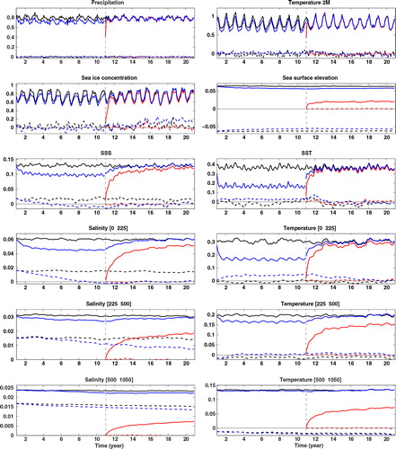
EnKF-SST shows smaller RMSE than FREE for all quantities investigated, although the improvement is sometimes small (Fig. 2). The initial reduction of error is faster for variables closer to the surface than in the deep water. It is also faster for temperature than for other variables. For instance, the error reduces rapidly for SST (within 2–3 months) and remains stable for the whole analysis period, while for salinity at 500–1000 m the error is still decreasing at the end of the analysis period, suggesting that a longer analysis period may be beneficial. Although the RMSE is decreased for all quantities, it is not always the case for bias, which becomes larger in some cases – for example for the surface and near surface temperatures. It was also found that if assimilation is continued beyond a 10-yr period, certain problems (mentioned in Section 3) introduce a drift in salinity and temperature at intermediate depth.

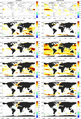
Fig. 3 Averaged differences between monthly RMSE in FREE and EnKF-SST, over the 10 analysis cycles. Warm colours indicate that the RMSE in the EnKF is smaller than in FREE. The units are the same as in Table 1.

Table 1 presents the error for FREE and Reduction of RMSE (RRMSE, in %) for EnKF-SST relative to FREE [see eq. (6)], which are quantified for the last year of the analysis period over the 10 cycles. For the 3-D hydrography, the reduction of error near the surface is about 25% for salinity and about 40–50% for temperature. The reduction of error is about 10% at intermediate depth and approximately 5% in the deep part of the ocean. The reduction of error is about 10% for sea level. For sea ice concentration, T2M and precipitation, benefits are approximately 10% and are the direct consequence of the improved ocean in the coupled system because these are not updated during assimilation.6

Table 1. The first column is the monthly RMSE calculated over the whole domain for FREE for the last year of the analysis period averaged over the 10 analysis cycles. The second column shows the corresponding improvements of EnKF-SST relative to FREE [RRMSE given in %; see eq. (6)]

RMSEFREE	RRMSEEnKF-SST (%)
T2M (°C)	0.82	11
Precip (mm/day)	0.79	9
ssh (m)	0.06	10
icec (%)	0.8	11
sst (°C)	0.36	54
sss (psu)	0.13	25
T[0 225] (°C)	0.31	45
S[0 225] (psu)	0.06	25
T[225 500] (°C)	0.16	15
S[225 500] (psu)	0.03	11
T[500 1050] (°C)	0.13	3
S[500 1050] (psu)	0.02	5

Figure 3 shows the spatial distribution of the difference between the RMSE in FREE and the EnKF-SST computed for the full analysis window and averaged over the 10 cycles. This allows us to locate areas where the main reduction of error occurs:

• Improvements in ice concentration are located at the ice edge, in areas where it has the largest variability.

• Benefits in sea level are mainly located in the Western Pacific Ocean and at the exit of the Indonesian Through-flow in the Southern Indian Ocean. Sea level is influenced indirectly by the update of heat content (positively via the thermosteric effect), salt content (negatively via the halosteric effect) and changes in the circulation pattern (barotropic current and resultant adjustment). Most of the improvements are the consequence of a reduction of the spatial sea level bias (Fig. 2).

• Benefits for SST are noticeable in areas where observations are assimilated (everywhere except in ice-covered water) and are strongest in areas where SST has large natural variability, that is, near the Equator, in the large conveyor current system and near the ice edge. Note that the error is larger than the observation error because RMSE is calculated from a monthly average and the error grows between the assimilation cycles.

• Benefits for sea surface salinity are mainly located near the equatorial Western Pacific and appears associated with a better-constrained precipitation field. Note that there is a weak degradation for salinity in the Baltic Sea, though both ice concentration and SST are improved. Updating hydrography without updating ice concentration during assimilation may introduce some bias. When EnKF-SST places sea ice in areas where TRUTH has none, hydrography is changed during analysis but ice concentration remains. Once the model is restarted, the ice melts and additional fresh water is released in the ocean. We suspect that this problem is visible only there, because of the weak exchange with the exterior. In future versions of NorCPM, a combined update of ice quantities will be considered.

• Near surface (between 0 and 225 m) benefits for hydrography are comparable to those observed for the surface, but with smaller amplitude.

• At intermediate depth (225–500 m), the benefits of hydrography are located in areas where the signature of SST extends to such depths, e.g. in the Circumpolar Currents and in the extension of the Gulf Stream. There is also a pronounced benefit in the Nordic Seas. Improvements may relate to a combined improved Atlantic Water inflow and improved surface water, which in turn leads to improved intermediate and deep water masses via convection.

• In the deep water the benefits in hydrography are only found in a few places. The scarcity of the improvements explains the small overall contribution in Table 1. Similarly to intermediate water, there are improvements in the Nordic Seas. There is also a maximum error reduction located at the deep outflow of the Mediterranean Sea in our model. Improved properties of the surface and intermediate water in the Mediterranean Sea may influence the outflow. Some weak degradation is noticed in the Atlantic (for example in the Caribbean Current).

• Benefits for precipitation occur near the tropics as a consequence of capturing ENSO SST variations, but no impacts are visible on land. Benefits for T2M are similar to that observed in SST with a smaller amplitude. Small benefits are noticed over land in Alaska, Scandinavia, and at the boundary between Canada and USA. Future versions of NorCPM may consider an update of the atmosphere flux, as in Zhang et al. (2009) and Zheng and Zhu (2010a), which may benefit the atmospheric component of the system.

5.2. Indices

This section analyses the ability of EnKF-SST to control SST and ocean circulation indices during the analysis phase. In contrast to SST, which has been measured for the past 100 yr, most ocean circulation indices are poorly observed. Indices considered here include the AMOC, the SPG, the Sub Tropical Gyre (STG), the Atlantic Multi-decadal Oscillation (AMO), and the Niño3 index. Note that the sample size on which correlations are computed is (100), so that correlations can be considered as significant above 0.17 (with a p-value of 0.05). The skill of FREE is zero and is not shown.

AMOC indices measure the maximum monthly transport value at a given latitude. The choice of the latitude is somewhat arbitrary. Pohlmann et al. (2009) and Swingedouw et al. (2012) use 48°N while Matei et al. (2012) and Dunstone et al. (2011) estimate the AMOC at lower latitudes (respectively 26.5° and 30°N) at 1000 m depths. Zhang et al. (2009) use the maximum of the transport within a 40–70°N latitude band. AMOC variability is controlled by the atmospheric circulation (local and remote), through momentum and buoyancy changes, including changes in the formation of NA water masses (Kuhlbrodt et al., 2007). By initialising the ocean, one can expect to improve the signal relative to the slow adjustment of the water masses, but not the signal related to unpredictable atmospheric variability. A common approach is to filter out the influence related to the atmosphere by applying a running mean on the time series. However, there is no consensus regarding the optimal time-window. Dunstone et al. (2011) use a 5-yr running mean while Swingedouw et al. (2012) use a 3-yr running mean. Figure 4 compares the correlation of AMOC in EnKF-SST with that of TRUTH, depending on the latitude and the length of the time averaging window. South of 40°N, correlations are barely significant while to the north, the correlations are stable and reach a maximum of 50–60°N. Correlations increase and are more stable with respect to latitude when a 5-yr running mean is used. In the following, we have retained the latitude 42°N (vertical dashed line in Fig. 4) because it corresponds to the core of variability in the leading mode of the meridional overturning. A time series of the AMOC index in EnKF-SST and TRUTH is presented in Fig. 5, and the correlation coefficient is reported in Table 2 for yearly frequency values and with a 5-yr running mean. Significant correlations are found for both timescales. The system seems to be less accurate between year 40 and 80 than at the starting and ending period. During this period, the AMOC in TRUTH is not found within the quartile envelope of EnKF-SST. It coincides with the period when the mean value in TRUTH is lower than normal and lower than that of the initial ensemble used in EnKF-SST. Although trends are reasonably well represented, there is a clear offset in the EnKF-SST. We suspect that EnKF-SST is not able to constrain both the trend and the offset within a 10-yr analysis period. It suggests that the correlation may improve if the analysis period was longer/continuous instead of being reinitialised at the beginning of each analysis cycle. The ensemble spread does not appear to reduce within the 10-yr analysis period.

Fig. 4 Correlation between the AMOC in EnKF-SST and TRUTH depending on the latitude. The blue line represents the correlation for the yearly time series. The black and red lines are the correlations when a 3- and 5-yr running mean is applied before calculating the correlation. The vertical dashed line indicates the 42°N latitude for which AMOC is calculated in Figures 5 and 7.

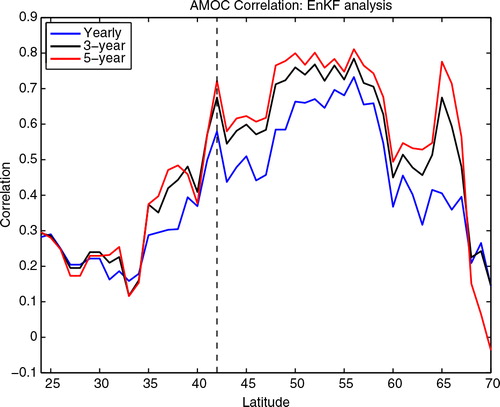
Fig. 5 Time series of the AMOC, the SPG, the STG and the AMO over the 10 analysis cycles for TRUTH (black) and EnKF-SST (blue). The blue shading is the ensemble quartile envelope and the blue line is the ensemble mean. For the AMOC, the bold line is the 5-yr running mean while the thin line represents the yearly values. The vertical dashed lines separate each of the analysis cycles.

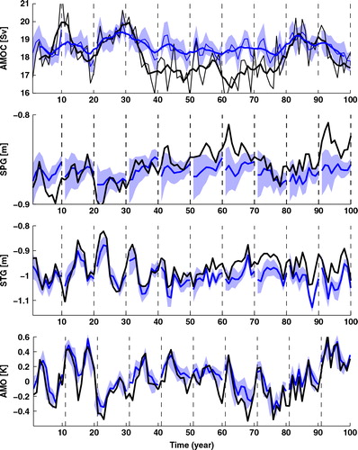
Table 2. Correlations between EnKF-SST and TRUTH over the 100-yr analysis period for the different indices

Corr EnKF
AMOC 42°	0.61
AMOC 42° (5-yr)	0.77
STG	0.82
SPG	0.59
AMO	0.93
Niño3	0.96

The SPG strength is plotted in the second panel of Fig. 5. The quantity is computed as proposed in the CORE2-protocol, that is, as the mean of sea level in the box (longitude [16–60°W]; latitude [48–65°N]). Note that a model bias of 7 cm was removed for plotting. The correlation of EnKF-SST with TRUTH is approximately 0.6. The performance of each analysis cycle is unequal. The ensemble used to initialise the analysis cycle samples a long period of the control run and is thus centred on the climatological mean of the system. If the analysis cycle starts when TRUTH is close to its climatological mean (in cycles 1, 2, 4, 5, 8 and 9), the assimilation only needs to maintain the evolution of the system. Otherwise (in cycles 3, 6, 7 and 10), the assimilation also needs to adjust for the initial offset. In such a case, the adjustment is slower, although the system usually improves during the analysis cycle. There is a clear reduction of the ensemble spread during the analysis cycle.

The third panel of Fig. 5 represents the STG index computed as proposed in the CORE2-protocol, that is, as the mean of sea level in the box (longitude [30–80°W]; latitude [30–45°N]). Note that a model bias of 0.15 cm was removed for plotting. Here, the fit is good with a correlation of 0.82 suggesting that assimilation of SST is able to control the yearly variability of sea level in the STG region.

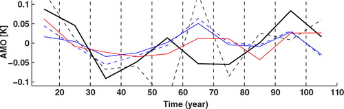
The fourth panel is the AMO index, which is defined here as the yearly averaged SST anomaly in the area (longitude [7–75°W]; latitude [0–60°N]). Although SST is assimilated in the model, some discrepancies are noticeable (see Table 2). One should bear in mind that observations are perturbed and that assimilation is done only once a month.

Niño3 index is the average of monthly SST anomaly in the area (longitude [90–150°W]; latitude [5°S–5°N]). Time series of the Niño3-index are not presented for the analysis period because discrepancies with TRUTH are too small to be visible. The corresponding correlation is high (see Table 2).

6. Prediction

6.1. Global state

In Section 5.1, EnKF-SST shows improvements compared to FREE for T2M, precipitation, ice concentration, sea level and 3-D hydrography during the analysis period. In this section, we investigate the skill of EnKF-SST in the prediction phase (year 11–20 in Fig. 2). As expected, the error increases with time for EnKF-SST and PERFECT, as observations are no longer used. It is satisfactory to notice that the error in EnKF-SST seldom exceeds that of FREE and if so, the degradation is small. This indicates that EnKF-SST conserves the equilibrium of the system appropriately and that biases introduced during the analysis period are small. The prediction of EnKF-SST is assessed for two periods: 1-yr averaged lead-time (henceforth referred to as ) and 2–5-yr averaged lead-time (henceforth referred to as ). As in Section 5.1, benefits are estimated quantitatively in Table 3 and compared to FREE using eq. (6).

Table 3. The first two columns are the 1 and 2–5 lead-year averaged RMSE, calculated over the whole domain for FREE. The remaining columns show the corresponding improvements for EnKF-SST and PERFECT relative to FREE [RRMSE given in %; see eq. (6) for each of the time-periods considered]

RMSEFREE		RRMSEEnKF (%)		RRMSEPERFECT (%)
Prediction year
T2M (°C)	0.55	0.37	7	4	13	7
Precip (mm/day)	0.48	0.26	11	5	19	10
ssh (m)	0.05	0.05	11	10	85	83
icec (%)	0.8	0.6	4	5	29	19
sst (°C)	0.3	0.2	21	8	39	18
sss (psu)	0.1	0.09	15	4	56	30
T[0 225] (°C)	0.21	0.19	22	5	54	25
S[0 225] (psu)	0.05	0.05	18	6	73	45
T[225 500] (°C)	0.16	0.16	11	4	74	51
S[225 500] (psu)	0.03	0.03	11	7	84	66
T[500 1050] (°C)	0.12	0.12	3	0	85	72
S[500 1050] (psu)	0.02	0.02	5	4	92	84

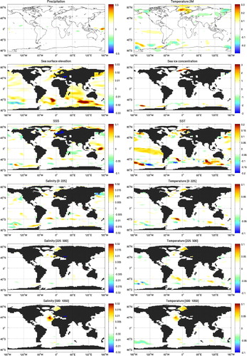
Fig. 6 The difference of 1 lead-year averaged RMSE of FREE and EnKF-SST, over the 10 prediction cycles, as in Figure 3.

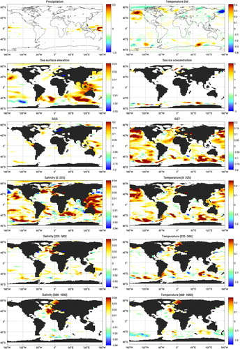
Fig. 7 The difference of 2–5 lead-year averaged RMSE of FREE and EnKF-SST, over the 10 prediction cycles, as in Figure 3.

EnKF-SST shows positive RRMSE for all variables studied both at and . The spatial reduction of error for EnKF-SST compared to FREE is presented in Fig. 6 for and in Fig. 7 for . Unlike in Fig. 3, the seasonal variability is removed by the yearly/multi-year averaging.

• For precipitation and T2M during , the improvements are about 5 and 10%. This is about half of what is found in PERFECT for which the atmosphere is perfectly initialised. This supports the idea that most of the predictability resides in the ocean. For T2M, patches of positive and negative RRMSE alternate with the positive RRMSE dominating. For precipitation, there are some clear improvements in the tropical Pacific and a weak global degradation. We suspect that the latter originates from the fact that coupled assimilation of atmospheric fluxes are not considered. For , quantitative improvements for T2M and precipitation are about 5%, which is still about half of what is found in PERFECT. For T2M, most of the benefits are located over Scandinavia and the Arctic. For precipitation, improvements remain limited to the tropic and are relatively small and restrained.

• For sea ice concentration, benefits of EnKF-SST compared to FREE remain quantitatively comparable for and with an error reduction of about 5% compare to FREE. Such a reduction is approximately 4–5 times smaller than what is found in PERFECT. At , positive and negative patches of RRMSE are observed with the positive dominating. For , the areas of negative RRMSE are few, and maximum predictability is found at the ice edge in the Nordic Seas.

• For sea level, benefits of EnKF-SST over FREE are stable for the two periods considered (about 10%). At , benefits are largest in the Western Pacific and in the Indian Ocean for .

• For temperature and salinity, the benefits of EnKF-SST over FREE for are: 20% near the surface, 10% at intermediate depth and 5% at deeper levels. For , benefits are reduced to about 5% at all depths. It is found that benefits remain longer at depth (in PERFECT and EnKF-SST) because of reduced mixing. It is also found that benefits in salinity persist longer than for temperature, probably because heat exchange occurs faster than salt exchange. Overall, PERFECT displays notably better skill than EnKF-SST. This is expected because in PERFECT, the neighbouring layers and atmosphere are perfectly initialised and SST is initialised with a lower observation error than for EnKF-SST. Nevertheless, a broader observation network may allow for further improvements.

6.2. Indices

This section presents prediction skills of the indices considered in Section 5.2. The prediction skills are calculated with respect to lead year in the prediction cycle. The predictability of EnKF-SST is compared against that of PERFECT and PERSISTENCE. FREE is again not presented because it has no skill. For yearly (resp. monthly) prediction indices: SPG, STG, AMO (resp. Niño3), PERSISTENCE are computed as the averaged observations of the last year (resp. month) prior to the prediction period.

Figure 8 presents the time series for each of the predictors for the 10 cycles. Correlations relative to the forecast lead-time (in years) are calculated. EnKF-SST is not considered successful if correlations are below the significance level or smaller than in PERSISTENCE. Correlations at a given lead-time are calculated from only 10 values. Correlations are significant above 0.5 with a p-value of 0.10, which makes the interpretation uncertain. In order to make the correlation estimation less sensitive to the sampling issue, the mean of the sample is replaced by the mean over the full time series. This can be done because the two estimators of the mean cover the same period of time and because the mean of the yearly value and the mean of every 10th value would converge to the same value for a sufficiently long time series. Such calculations are used in Pohlmann et al. (2009) [their eq. (1)].

Fig. 8 Left panels: time series of different indices are on the left column. Right panels: the correlation relative to the forecast lead-time (in years). Vertical dashed lines separate each of the prediction cycles. The black line is TRUTH, the red line is PERFECT, the blue line is EnKF-SST and the horizontal dashed line is PERSISTENCE. The dashed blue line for the SPG index in the right panel represents the skill of the EnKF-SST when the initial bias is corrected as in PERSISTENCE.

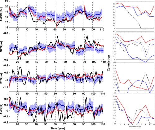
For the AMOC time series, a 5-yr running mean of TRUTH is plotted while the other lines correspond to yearly ensemble means of EnKF-SST and PERFECT. The motivation for using a running average is that year-to-year variability is mainly driven by fast atmospheric processes (such as related to the NAO), which is mostly removed when using ensemble averaging. In order to have comparable variability to TRUTH, PERSISTENCE uses a 5-yr average, which is centred on the year prior to the start of the prediction periods. As such, PERSISTENCE uses observations from the future (up to year 2). Therefore, a dotted black line is used during this period of time in the correlation plot. For PERSISTENCE, the correlation drops below 0.4 after 3–4 yr of prediction, while both EnKF-SST and PERFECT match the variability in TRUTH up to a 10-yr lead-time reasonably well. PERFECT and EnKF-SST follow the trends in TRUTH reasonably well. Predictions in EnKF-SST are better when the initial starting point of the prediction is not too far from TRUTH. In such a case, TRUTH lies within the quartile envelope. Although PERFECT performs better than EnKF-SST, their skill is comparable, suggesting that SST may be sufficient to constrain low frequency variability of AMOC when 3-D and multivariate updates are used.

For the SPG time series, none of the prediction systems are capable of representing the year-to-year variability seen in TRUTH. PERSISTENCE provides a reasonable predictability (correlation of approximately 0.5) up to a 10-yr lead-time resulting from the multi-decadal variability seen in TRUTH. Similarly to AMOC, PERFECT and EnKF-SST follow trends observed in TRUTH reasonably well, but EnKF-SST is poorer than PERSISTENCE (in regard to correlation). This is caused by the offset at the start of the prediction cycle. In Section 5.2, it was found that EnKF-SST was not capable of accurately constraining the mean value of SPG. Another prediction (with a dashed blue line in the correlation) was attempted, where the bias observed in the year prior to the prediction period was removed. It implies that the blue lines in the time series are shifted to the start of PERSISTENCE (horizontal dashed line) at each cycle. Up to year 6, this predictor beats PERSISTENCE implying that trends in EnKF-SST have some skill. However, the skill is still not as good as in PERFECT and more observations seem necessary to improve the prediction skill. PERFECT has prediction skill up to a 10-yr lead-time.

For the STG, TRUTH shows higher frequency variability than for previous indices. Although the STG index seemed to be controlled well during the analysis period, both PERFECT and EnKF-SST are almost flat during the prediction period. No predictability is found beyond a 1-yr lead-time (PERSISTENCE shows no correlation at 1-yr lead-time while that of EnKF-SST is barely significant).

Similarly to STG, the AMO index shows higher frequency than decadal variability. The correlations are not significant for any of the predictors beyond a 2-yr lead-time. The correlation seems comparable for the three predictors (although PERFECT may be slightly better) suggesting that auto-correlation is the main reason for the correlation. It should be noted that EnKF-SST and PERFECT show weaker variability than TRUTH because of ensemble averaging. Earlier studies (Griffies and Bryan, 1997; Boer, 2000; Collins et al., 2006) suggested that an accurate initialisation of MOC might allow prediction of AMO a decade or more in advance. However, Medhaug and Furevik (2011) show that this relationship is model dependent and it is possible that the coarse resolution of our system may have an impact. In order to enhance the multi-decadal properties of the index, decadal-averaged predictions (i.e. the average of the prediction cycles) of AMO are shown in Fig. 9. The correlations are relatively low for all predictors, with 0.54 for PERFECT, 0.37 for PERSISTENCE and 0.37 for EnKF-SST. If the offset prior to the start of the prediction is corrected in EnKF-SST, the correlation reaches 0.51 (plotted with the dashed blue line in the correlation plot). Such correlations are at the edge of statistical significance and no firm conclusion can be drawn.

Fig. 9 Time series of the detrended decadally averaged AMO index for TRUTH (thick black line), PERFECT (red line), EnKF-SST (blue line), PERSISTENCE (dashed black line) and EnKF-SST if initial bias is corrected (dashed blue line). Vertical dashed lines separate each of the prediction cycles.

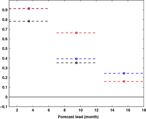
Predictions of Niño3 are analysed for three periods: 1–6 months, 6–12 months and 12–18 months lead-time (see Fig. 10). Correlations are computed from 6-month averages in order to limit the impact of monthly variability. During the first 6-months, EnKF-SST and PERFECT provide improved prediction skill compared to PERSISTENCE with a correlation of approximately 0.9. On the following time period (6–12 months), the prediction skill reduces rapidly for EnKF-SST and PERSISTENCE to approximately 0.4 as a response to the spring predictability barrier (Zheng and Zhu, 2010b) while that of PERFECT remains relatively high (0.7). Prediction skill over 1-yr is very small in EnKF-SST and PERFECT (approximately 0.2 that is below statistical significance) and no prediction is evident in PERSISTENCE.

Fig. 10 Correlation with the Niño3 index for PERSISTENCE (black), PERFECT (red) and EnKF-SST (blue). Correlations are computed for 6-month averages. For the first 6 months, EnKF-SST is under PERFECT.

6.3. A regional case: the Nordic Seas

The RMSE distributions of various climatic parameters indicate that the model predictability is not uniformly distributed in space (Figs. 6 and 7). This section offers a closer, albeit tentative, look at the predictive skill in the Nordic Seas, a region that stands out with particularly high prediction score in our model.

Figure 11 shows that NorESM simulates inter-annual to multi-decadal temperature variability along the path of the Atlantic Water to the Arctic. A common picture for the Nordic Seas is that the EnKF-SST forecast outperforms PERSISTENCE and is close to PERFECT. In some cases PERSISTENCE is initially doing better than EnKF-SST because the initial starting point is slightly off compare to TRUTH. A comparison of the individual sub-regions reveals some interesting spatial differences. While a northward propagation of signals is only discernible in the last cycle, there is a clear change from the dominance of sub-decadal variability in the southern part (Fig. 11d, e) to multi-decadal variability in the northern part of the Nordic Seas (Fig. 11a–c). This change is also reflected in the respective correlation scores (Fig. 11i–h). In the southern part, the skill of the persistence forecast drops sharply during the first 3–4 yr (Fig. 11i, j, black curve), indicating only weak auto-correlation. The skill decline is slower for EnKF-SST and PERFECT, which account for 25–65% of the variance during the first 5 yr and approach zero towards the end of the forecast cycle. The EnKF-SST prediction skill is somewhat lower than for PERFECT, in particular on inter-annual (<4 yr) and near-decadal (6–8 yr) time scales, indicating that the assimilation of more data could further improve the predictions. In the northern part, the effect of auto-correlation lasts longer and the skill of the persistence forecast decreases almost linearly over the duration of the forecast cycle (reaching 0.2 after 10 yr). The skills for EnKF-SST and PERFECT remain high over the entire cycle (reaching 0.6–0.8 after 10 yr) and the benefit from assimilation (i.e. the difference between EnKF-SST and PERSISTENCE) grows as the forecast lead increases.

Fig. 11 Prediction of heat content (0–300 m) in different regions of the Nordic Seas. The thick black line is TRUTH, the dashed black line is PERSISTENCE, the red line is PERFECT and the blue line is EnKF-SST. Shaded areas correspond to the quartile envelope. Vertical black lines separate each of the prediction cycles.

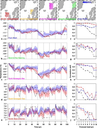
In summary, EnKF-SST shows good predictive skill in the Nordic Seas. This result indicates that: (1) there is a benefit of having a dynamical prediction – as opposed to static prediction (PERSISTENCE) – system for this region; and (2) a significant fraction of the predictive potential can be exploited with assimilation of SST data alone. In the Southern part of the Nordic Seas (South Norwegian Sea and Nordic Sea entrance) potential predictability is of approximately 5 yr, whereas decadal predictability is achieved further north.

7. Conclusion and discussions

This study provides: (1) a reassessment of the use of SST data for seasonal-to-decadal prediction using a more advanced scheme compared to previous studies (that used relaxation); and (2) further demonstration of the potential use of the advanced EnKF data assimilation with full ocean state update for such predictions. The study utilised twin experiments, allowing an in-depth assessment of the impact of our data assimilation method for all model variables. We assume a perfect model and thus our results provide an upper bound for the skill of our system. However, we employ a numerically efficient coarse resolution version of NorCPM, and our results may not be representative of other models. NorCPM is tested for 10 cycles, each consisting of a 10-yr assimilation phase, followed by a 10-yr prediction.

Over a 100-yr period of study, data assimilation reduces error for all quantities investigated – sea level, ice concentration, T2M, precipitation and 3-D hydrography – during the analysis phase and prediction phase up to a 5-yr lead-time. Benefits are largest near the surface but last longer at depth. Benefits are largest for temperature but last longer for other quantities (salinity, sea level and ice concentration). These results encourage the use of ensembles to derive 3-D multivariate updates as more information can be exploited from sparse observations.

The system is tested for standard indices over sufficiently long periods to cover ascending, descending, and transient phases of the indices. It is hard to place our results among existing literature because skill may vary depending on: the model system used, whether varying external forcing are used or not and if the system is tested in twin experiments or in a realistic framework. The system shows predictability for heat content in the Nordic Seas, the SPG and the overturning circulation (AMOC) in the North Atlantic for up to 10-yr lead-time and is better than PERSISTENCE. It shows lower skill than PERFECT for the SPG but has nearly comparable skill for the heat content in the Nordic Seas and the AMOC. However, the system seems to have limitations in constraining trends and adjusting biases simultaneously over an analysis cycle of 10 yr. The possible reasons are that: SST is insufficient to fully constrain the system; the analysis period (currently 10 yr) should be extended to better synchronise the model with the truth; the assimilation window (currently 1 month) is not appropriate and coupled assimilation of atmosphere and ice variables should be considered. Each of these options is now discussed.

Reducing the assimilation window is possible if the observation error variance is increased accordingly, in order to maintain the equilibrium between model and observational accuracy. This may lead to a closer match with observations because the system would undergo smaller updates reducing error due to the linear approximation during the analysis and because the finite ensemble size would span the fewer non-linearities developed during a shorter period of time more appropriately. However, reducing the assimilation window is more costly as the system needs to be stopped for each assimilation cycle; the contribution from mesoscale variability would become larger than with monthly average observations, and finally, linear time interpolation of the observations would become necessary (100-yr SST are provided at monthly frequencies only).

A broader observation network would improve the prediction skill of our system. Prediction in PERFECT (for which the full model state is observed) shows improved skill compare to the EnKF-SST prediction system. Zhang et al. (2009); Dunstone et al. (2011) demonstrate the improvements when Argo floats are included. Real-time forecasting systems assimilating altimetry data, (e.g. Sakov et al., 2012), indicate that it has a strong potential to constrain effectively the SPG and the branching of Atlantic Water into the Nordic Seas. Assimilation of ice concentration has potential for constraining ice properties (Lisæter et al., 2003; Sakov et al., 2012). In future, NorCPM may use a wide observation network as in the TOPAZ system (Sakov et al., 2012), which assimilates: SST, altimetry, Argo float observations, ice concentration and ice drift.

In this study, each of the 10 analysis cycles are initialised from a random sampling of the control run and assimilated for 10 yr. This analysis period seems too short as the errors in the deep are still reducing at the end of the analysis cycle for some quantities. For the SPG index, the adjustment is slow and the system seems more accurate at the end of the analysis period compared to the beginning. This suggests that the system would benefit by reinitialising from the previous cycle. However, a weak trend is noticed for some variables when assimilation is done over periods longer than 10 yr (not shown). This drift originates from the way empty layers are handled during assimilation. An alternative where assimilation corrects for heat content, salt content and layer thickness rather than temperature, salinity and layer thickness will be investigated in future works.

The primary goal of NorCPM is to provide reliable prediction for the Nordic countries both on land and at sea. The current system has a high skill (close to the maximum predictability) for heat content in the Nordic Seas. Improved heat flux in the area led to some skill for ice concentration and atmospheric temperature around Scandinavia up to a 5-yr lead-time. Although these results are encouraging, a test of the system should be conducted in a realistic framework before drawing any firm conclusions relating to its accuracy.

The current system was tested in the framework of twin-experiments. This approach is practical because it allows for extensive testing of the accuracy of the system and assumes that the model is bias free. Biases in data assimilation are problematic because most methods assume that the model and observations are bias free (Dee, 2005), while biases in climate models are large because of their coarse resolution. A practical way to handle this problem in the climate community was to assimilate anomalies instead of the data itself (Keenlyside et al., 2008; Smith et al., 2008; Pohlmann et al., 2009; Dunstone et al., 2011; Swingedouw et al., 2012). However, in most systems biases are not static and may vary seasonally/inter-annually. The EnKF can estimate biases by augmenting the model state (Dee, 2005; Sakov et al., 2012). Future configuration of NorCPM may consider this approach.

Finally, many examples show the advantage of using coupled assimilation with atmospheric fluxes (Zhang et al., 2009; Zheng and Zhu, 2010a). Further studies may consider coupled assimilation of ice properties and atmospheric fluxes.

8. Acknowledgments

This study was partly funded by the Centre for climate dynamics at the Bjerknes Centre and the Norwegian Research Council under the NORKLIMA research project (EPOCASA; 229774/E10). This work has also received a grant for computer time from the Norwegian Program for supercomputing (NOTUR2, project number nn2993k). We would like to thank B. Backeberg and P. Raanes for their valuable comments.

Notes

¹Note that the statistic for T2M and precipitation are computed from only nine cycles because data from one of the cycle were lost.

²However, we did not test this system due to technical reasons, see Section 3.

³Observation error in EnKF-SST is 0.1°C whereas in PERFECT it is 1×10⁻⁶°C.

⁴PERSISTENCE is the yearly average prior to the start of the prediction. A 10-yr average was also attempted but reached poorer skill.

References

- Anderson J . An Ensemble Adjustment Kalman Filter for data assimilation. Mon. Weather. Rev. 2001; 129(12): 2884–2903.
- Assmann K. M. , Bentsen M. , Segschneider J. , Heinze C . An isopycnic ocean carbon cycle model. Geosci. Model Dev. 2010; 3(1): 143–167.
- Bengtsson L. , Semenov V. A. , Johannessen O. M . The early twentieth-century warming in the Arctic–a possible mechanism. J. Clim. 2004; 17(20): 4045–4057.
- Bentsen M. , Bethke I. , Debernard J. B. , Iversen T. , Kirkevåg A. , co-authors . The Norwegian Earth System Model, NorESM1-M – Part 1: description and basic evaluation of the physical climate. Geosci. Model Dev. 2013; 6: 687–720.
- Bertino L. , Evensen G. , Wackernagel H . Sequential data assimilation techniques in oceanography. Int. Stat. Rev. 2003; 71(2): 223–241.
- Bitz C. , Holland M. , Hunke E. , Moritz R . Maintenance of the sea-ice edge. J. Clim. 2005; 18(15): 2903–2921.
- Bleck R. , Rooth C. , Hu D. , Smith L. T . Salinity-driven thermocline transients in a wind – and thermohaline – forced isopycnic coordinate model of the North Atlantic. J. Phys. Oceanogr. 1992; 22: 1486–1505.
- Boer G . A study of atmosphere-ocean predictability on long time scales. Clim. Dynam. 2000; 16(6): 469–477.
- Boer G. J . Long time-scale potential predictability in an ensemble of coupled climate models. Clim. Dynam. 2004; 23(1): 29–44.
- Branstator G. , Teng H . Two limits of initial-value decadal predictability in a CGCM. J. Clim. 2010; 23(23): 6292–6311.
- Branstator G. , Teng H. , Meehl G. , Kimoto M. , Knight J. , co-authors . Systematic estimates of initial-value decadal predictability for six AOGCMs. J. Clim. 2012; 25(6): 1827–1846.
- Brusdal K. , Brankart J. , Halberstadt G. , Evensen G. , Brasseur P. , co-authors . A demonstration of ensemble-based assimilation methods with a layered OGCM from the perspective of operational ocean forecasting systems. J. Mar. Syst. 2003; 40: 253–289.
- Collins M. , Botzet M. , Carril A. , Drange H. , Jouzeau A. , co-authors . Interannual to decadal climate predictability in the North Atlantic: a multimodel-ensemble study. J. Clim. 2006; 19(7): 1195–1203.
- Counillon F. , Bertino L . Ensemble Optimal Interpolation: multivariate properties in the Gulf of Mexico. Tellus A. 2009; 61(2): 296–308.
- Dee D. P . Bias and data assimilation. Q. J. Roy. Meteorol. Soc. 2005; 131(613): 3323–3343.
- Dunstone N. , Smith D. , Eade R . Multi-year predictability of the tropical Atlantic atmosphere driven by the high latitude North Atlantic Ocean. Geophys. Res. Lett. 2011; 38(14): L14701.
- Evensen G . The Ensemble Kalman Filter: theoretical formulation and practical implementation. Ocean. Dynam. 2003; 53(4): 343–367.
- Frankcombe L. M. , Von Der Heydt A. , Dijkstra H. A . North Atlantic multidecadal climate variability: an investigation of dominant time scales and processes. J. Clim. 2010; 23(13): 3626–3638.
- Gent P. , Danabasoglu G. , Donner L. , Holland M. , Hunke E. , co-authors . The community climate system model version 4. J. Clim. 2011; 24(19): 4973–4991.
- Griffies S. M. , Bryan K . Predictability of North Atlantic multidecadal climate variability. Science. 1997; 275(5297): 181–184.
- Han G. , Tang C . Interannual variations of volume transport in the western Labrador Sea based on TOPEX/Poseidon and WOCE data. J. Phys. Oceanogr. 2001; 31(1): 199–211.
- Haugen V. E. , Evensen G . Assimilation of SLA and SST data into an OGCM for the Indian Ocean. Ocean. Dynam. 2002; 52(3): 133–151.
- Hawkins E. , Sutton R . The potential to narrow uncertainty in regional climate predictions. Bull. Am. Meteorol. Soc. 2009; 90(8): 1095–1107.
- Holliday N. P. , Hughes S. , Bacon S. , Beszczynska-Möller A. , Hansen B. , co-authors . Reversal of the 1960s to 1990s freshening trend in the northeast North Atlantic and Nordic Seas. Geophys. Res. Lett. 2008; 35(3): L03614.
- Jones P. , New M. , Parker D. , Martin S. , Rigor I . Surface air temperature and its changes over the past 150 years. Rev. Geophys. 1999; 37(2): 173–199.
- Jungclaus J. H. , Haak H. , Latif M. , Mikolajewicz U . Arctic–North Atlantic interactions and multidecadal variability of the meridional overturning circulation. J. Clim. 2005; 18(19): 4013–4031.
- Keenlyside N. , Latif M. , Botzet M. , Jungclaus J. , Schulzweida U . A coupled method for initializing El Nino Southern Oscillation forecasts using sea surface temperature. Tellus A. 2005; 57(3): 340–356.
- Keenlyside N. , Latif M. , Jungclaus J. , Kornblueh L. , Roeckner E . Advancing decadal-scale climate prediction in the North Atlantic sector. Nature. 2008; 453(7191): 84–88.
- Kirkevåg A. , Iversen T. , Seland Ø. , Hoose C. , Kristjánsson J. E. , co-authors . Aerosol-climate interactions in the Norwegian Earth System Model – NorESM. Geosci. Model Dev. Discuss. 2012; 5: 2599–2685.
- Krauss W. , Döscher R. , Lehmann A. , Viehoff T . On eddy scales in the eastern and northern North Atlantic Ocean as a function of latitude. J. Geophys. Res. Oceans. (1978–2012) . 1990; 95(C10): 18049–18056.
- Kuhlbrodt T. , Griesel A. , Montoya M. , Levermann A. , Hofmann M. , co-authors . On the driving processes of the Atlantic meridional overturning circulation. Rev. Geophys. 2007; 45(2), RG2001. ):
- Latif M. , Collins M. , Pohlmann H. , Keenlyside N . A review of predictability studies of Atlantic sector climate on decadal time scales. J. Clim. 2006; 19(23): 5971–5987.
- Lisæter K. A. , Rosanova J. , Evensen G . Assimilation of ice concentration in a coupled ice–ocean model, using the Ensemble Kalman filter. Ocean. Dynam. 2003; 53(4): 368–388.
- Loeng H. , Drinkwater K . An overview of the ecosystems of the Barents and Norwegian Seas and their response to climate variability. Deep Sea Research Part II: Topical Studies in Oceanography. 2007; 54(23): 2478–2500.
- Luo J.-J. , Masson S. , Behera S. , Shingu S. , Yamagata T . Seasonal climate predictability in a coupled OAGCM using a different approach for ensemble forecasts. J. Clim. 2005; 18: 4474–4497.
- Matei D. , Baehr J. , Jungclaus J. , Haak H. , Müller W. , co-authors . Multiyear prediction of monthly mean Atlantic meridional overturning circulation at 26.5°N. Science. 2012; 335(6064): 76–79.
- Medhaug I. , Furevik T . North Atlantic 20th century multidecadal variability in coupled climate models: sea surface temperature and ocean overturning circulation. Ocean Sci. 2011; 7: 389–404.
- Meehl G. A. , Goddard L. , Murphy J. , Stouffer R. J. , Boer G. , co-authors . Decadal prediction: can it be skillful?. Bull. Am. Meteorol. Soc. 2009; 90(10): 1467–1485.
- Otterå O. H. , Bentsen M. , Drange H. , Suo L . External forcing as a metronome for Atlantic multidecadal variability. Nat. Geosci. 2010; 3(10): 688–694.
- Parkinson C. L. , Cavalieri D. J . Arctic sea ice 1973–1987: seasonal, regional, and interannual variability. J. Geophys. Res. 1989; 94(C10): 14499–14523.
- Petoukhov V. , Semenov V. A . A link between reduced Barents-Kara sea ice and cold winter extremes over northern continents. J. Geophys. Res. 2010; 115(D21): D21111.
- Philander S. G . El Niño, La Niña, and the Southern Oscillation. 1990; Academic Press, San Diego, USA. 293.
- Pohlmann H. , Jungclaus J. , Köhl A. , Stammer D. , Marotzke J . Initializing decadal climate predictions with the GECCO oceanic synthesis: effects on the North Atlantic. J. Clim. 2009; 22(14): 3926–3938.
- Sakov P. , Counillon F. , Bertino L. , Lisæter K. , Oke P. , co-authors . TOPAZ4: an ocean-sea ice data assimilation system for the North Atlantic and Arctic. Ocean Sci. 2012; 8: 633–656.
- Sakov P. , Oke P . A deterministic formulation of the ensemble Kalman filter: an alternative to ensemble square root filters. Tellus A. 2008; 60(2): 361–371.
- Schweckendiek U. , Willebrand J . Mechanisms affecting the overturning response in global warming simulations. J. Clim. 2005; 18(23): 4925–4936.
- Shields C. A. , Bailey D. A. , Danabasoglu G. , Jochum M. , Kiehl J. T. , co-authors . The low-resolution CCSM4. J. Clim. 2012; 25(12): 3993–4014.
- Simon E. , Bertino L . Application of the Gaussian anamorphosis to assimilation in a 3-D coupled physical-ecosystem model of the North Atlantic with the EnKF: a twin experiment. Ocean Sci. 2009; 5(4): 495–510.
- Smith T. , Reynolds R. , Peterson T. , Lawrimore J . Improvements to NOAA's historical merged land-ocean surface temperature analysis (1880–2006). J. Clim. 2008; 21(10): 2283–2296.
- Srinivasan A. , Chassignet E. , Bertino L. , Brankart J. , Brasseur P. , co-authors . A comparison of sequential assimilation schemes for ocean prediction with the HYbrid Coordinate Ocean Model (HYCOM): twin experiments with static forecast error covariances. Ocean. Model. 2011; 37(3): 85–111.
- Swingedouw D. , Mignot J. , Labetoulle S. , Guilyardi E. , Madec G . Initialisation and predictability of the AMOC over the last 50 years in a climate model. Clim. Dynam. 2012; 40(9–10): 2381–2399.
- Tatebe H. , Ishii M. , Mochizuki T. , Chikamoto Y. , Sakamoto T. T. , co-authors . The initialization of the MIROC climate models with hydrographic data assimilation for decadal prediction. J. Meteorol. Soc. Jpn. 2012; 90: 275–294.
- Taylor K. E. , Stouffer R. J. , Meehl G. A . An overview of CMIP5 and the experiment design. Bull. Am. Meteorol. Soc. 2012; 93(4): 485.
- Thacker W . Data assimilation with inequality constraints. Ocean. Model. 2007; 16(3): 264–276.
- Tjiputra J. F. , Roelandt C. , Bentsen M. , Lawrence D. , Lorentzen T. , co-authors . Evaluation of the carbon cycle components in the Norwegian Earth System Model (NorESM). Geosci. Model Dev. 2012; 5: 3035–3087.
- Vertenstein M., Craig T., Middleton A., Feddema D., Fischer C. CESM1.0.3 User Guide. 2012. Online at: http://www.cesm.ucar.edu/models/cesm1.0/cesm/cesm_doc_1_0_4/ug.pdf.
- Wittenberg A. T . Are historical records sufficient to constrain ENSO simulations?. Geophys. Res. Lett. 2009; 36(12): L12702.
- Zhang S. , Anderson J. , Rosati A. , Harrison M. , Khare S. P. , co-authors . Multiple time level adjustment for data assimilation. Tellus A. 2004; 56(1): 2–15.
- Zhang S. , Harrison M. , Rosati A. , Wittenberg A . System design and evaluation of coupled ensemble data assimilation for global oceanic climate studies. Mon. Weather. Rev. 2007; 135(10): 3541–3564.
- Zhang S. , Rosati A. , Delworth T . The adequacy of observing systems in monitoring the Atlantic meridional overturning circulation and North Atlantic climate. J. Clim. 2010; 23(19): 5311–5324.
- Zhang S. , Rosati A. , Harrison M . Detection of multidecadal oceanic variability by ocean data assimilation in the context of a “perfect” coupled model. J. Geophys. Res. 2009; 114(C12): C12018.
- Zhang Z. S. , Nisancioglu K. , Bentsen M. , Tjiputra J. , Bethke I. , co-authors . Pre-industrial and mid-Pliocene simulations with NorESM-L. Geosci. Model Dev. 2012; 5(2): 523–533.
- Zheng F. , Zhu J . Coupled assimilation for an intermediated coupled ENSO prediction model. Ocean. Dynam. 2010a; 60(5): 1061–1073.
- Zheng F. , Zhu J . Spring predictability barrier of ENSO events from the perspective of an ensemble prediction system. Global. Planet. Change. 2010b; 72(3): 108–117.
- Zwally H. J. , Comiso J. C. , Parkinson C. L. , Cavalieri D. J. , Gloersen P . Variability of Antarctic sea ice 1979–1998. J. Geophys. Res. 2002; 107(C5): 3041.