An intercomparison study of ice thickness models in the Netherlands

Abstract

Lake models account for the thermodynamic interaction between fresh water lakes and the atmosphere. During frost periods they predict ice thickness. A stand-alone version of the Fresh water Lake model (FLake) has been compared with the operational ice-growth model at the Royal Netherlands Meteorological Institute. Both models have been driven with various input data like observations and data from the Hirlam Aladin Research on Mesoscale Operational NWP In Europe (HARMONIE) model. The lake ice models are validated with indirect ice thickness measurements at Cabauw during the winter of 1996/1997 and with data from a voluntary observer network in the province of Friesland (The Netherlands) during the winter of 2012. FLake is shown to have predictive power and is competitive with the operational ice-growth model.

• ice thickness
• lake models
• FLake
• Cabauw
• validation

1. Introduction

There is a long tradition of ice skating in the Netherlands. Famous Dutch painters from the Golden age depicted ice skating on frozen waterways. Ice skating is still popular in the Netherlands. In cold spells numerous ditches, canals and lakes get frozen and many people go out for ice skating tours. During these periods, there is a great interest in ice thickness predictions at specific locations. The Royal Netherlands Meteorological Institute (KNMI) issues ice thickness predictions, based on a model of De Bruin and Wessels (1988; henceforth BW88). In the Netherlands, with its moderate climate the cold spells come and go, resulting in a growing and disappearing ice floor. This is in contrast with the Arctic and mountainous regions where ice floors may be present for more than 5 months. In those regions, ice floors are permanently covered with a thick snow layer, which make them unsuitable for ice skating. Lakes covered with ice interact with the atmosphere and their effect should be considered in mesoscale models. In this paper, we compare FLake with the BW88 model and with ice thickness observations. FLake (Mironov, 2008) is the Fresh water Lake parameterisation that is used to account for the effect of lakes in Numerical Weather Prediction (NWP) and climate models. The BW88 model has never been confronted with an accepted state-of-the-art lake model, which might offer an alternative opportunity to predict ice thickness in the Netherlands. In our study, we have selected two winters in which the 11-city tour, a major skating event, played an important role. In 1997, the 11-city tour took place while in 2012 it was almost organised. During those periods, ice thickness predictions are highly desirable. The first issue addressed in this paper is the performance of ice models using observations. These forcing contains only little instrumental errors and in this way we can focus on the performance of the lake models. We have used high-quality observations from Cabauw (the Netherlands) to drive the lake models and we also used observed water temperature profiles for evaluation. The second issue addresses regional ice thickness forecasts. Using meteorological input data produced by the Hirlam Aladin Research on Mesoscale Operational NWP In Europe (HARMONIE/AROME) model (Seity et al., 2011), we investigate if the lake ice models are capable of producing ice thickness at specific locations. For validation, we have used measurements from a voluntary observer network in the province of Friesland.

2. Short description of the lake ice models

2.1. KNMI operational ice-growth model

The operational ice-growth model at KNMI is a one-layer model and the entire water column is described by a single value of temperature (see BW88 for details). The predicted variables are water temperature, ice and snow thickness. Originally, the model was driven by SYNOPS observations, and therefore, special attention was given to an accurate estimation of the incoming short- and long-wave radiation (Holtslag and van Ulden, 1983). The following expression is used for the incoming short-wave radiation1 where Φ is the solar elevation and N is total cloud cover fraction. The incoming long-wave radiation is calculated according to2 where is the apparent emissivity of the atmosphere which depends on the temperature, σ is the Boltzmann constant, T is the 2 m temperature and is low cloud cover fraction. In a later stage, the BW88 model was also driven with NWP data but the calculation of the radiation components remained intact.

The differential equation which describes the build-up of an ice layer reads as3 where L _f is the latent heat for freezing, ρ _i is the density of ice, and H _i is the ice thickness. The term represents the total heat flux from the atmosphere, T _e is the equilibrium temperature, T _s is the surface temperature, and Q _w is the heat flux from the water to the ice. A is the aerodynamic exchange coefficient and is estimated in the ice build-up phase with4 where T _i is the wet bulb temperature at screen height and is the 10-m-wind speed. The equilibrium temperature T _e is calculated using the expression5 where is the net radiation. Q _w is calculated using6 where D is the lake depth. For further details, we refer to De Bruin and Wessels (1988). For the evolution of a snow layer above the ice layer, an extra term is added in eq. (3). This term contains the accumulated snow depth.

The accumulated snow depth h _s [m] is computed from precipitation data using7 where J is the present time-step, R _j is the snow water equivalent in (kg/m²/s) during the jth time-step after the first appearance of ice, and ρ _j is the corresponding snow density (kg/m³). The snow density is difficult to predict and depends on the type of snowfall, wind speed, solar heating and percolation of melting water or rain. It is estimated by8

where J is the present time-step and j is the secondary time-step which is updated after the first appearance of ice. Δt is the primary time-step which is in our case 12 h. Note that ρ _j , the snow density in (kg/m³) approaches the ice density and is therefore limited, that is, . The thermal conductivity and the albedo of snow are corrected for aging in a similar manner.

2.2. FLake

An offline version of the FLake model has been supplied by Leibniz Institute of Freshwater Ecology and Inland Fisheries (FLake). The FLake model is based on the concept of self-similarity of the thermal structure of the water column (Martynov et al., 2010). A two-layered water temperature profile is assumed, with the mixed layer at the surface and the thermocline extending from the lake bottom to the base of the mixed layer.

The water potential temperature θ(z, t) is given by9

where z is the depth, h is the mixed-layer depth, D is the lake depth, θ _s is the mixed layer temperature and θ _s is the bottom temperature. The thermocline, defined as10

can be parameterised using a fourth-order polynomial function of the depth, depending on the shape coefficient C _T ,11

as a function of dimensionless depth ,12

The value of the shape coefficient C _T lies between 0.5 and 0.8. This means that the thermocline can neither be very concave nor very convex. The same parametric concept is applied to the ice and snow layers with linear shape functions and also to the bottom sediment layer. Note that the assumption of linearity of the ice shape function is only valid for thin layers of ice, which is reasonable for the Netherlands with its moderate climate. The evolution in time of the ice thickness is described by13

L _f is latent heat for freezing, ρ _i is the density of ice, H _i is ice thickness, κ is heat conductivity, θ _f is the fresh-water freezing point, θ _i is the temperature at the air–ice interface, is the derivative of the shape function Φ _I with respect to the dimensionless vertical coordinate and Q _w is the heat flux water to ice and is estimated using14

is the bottom temperature. The above-mentioned differential equation is numerically solved. For details, we refer to (Mironov, 2008; Mironov et al., 2010). Updates of the code which improve the behaviour of the model (Semmler et al., 2012) with respect to the ice–snow–atmosphere interface have been implemented. Firstly, the snow density ρ _j is no longer a function of time anymore, but it is kept constant at a value of 320 (kg/m³). Consequently, the accumulated snow height can now be calculated in a similar fashion as BW88 [see formula (7)]. Secondly, the thermal heat conductivity is recalculated, with the effective conductivity k of an ice-covered lake given by15

with k _snow, k _ice the conductivity of the snow and ice, respectively, and h _s the snow depth. This correction simulates the influence of the snow cover inhomogeneities and decays with increasing snow depth. Thirdly, the albedos of snow and ice have been modified. Different estimates of the surface albedo with respect to solar radiation are used for dry and melting ice and snow,16

where α _melting for ice is 0.3, for snow 0.77 and α _dry for ice is 0.5, for snow 0.87, and a mixing parameter A(T _s ) defined as17

where T ₀ is the freezing temperature [K] and T _s is the surface temperature [K].

3. Set-up of external parameters, meteorological forcing and initialisation

In Table 1, the set-up parameters of the lake models are shown. Note that the geographical positions are also depicted in Fig. 8. Most of the lakes are shallow and the depth does not exceed values of 5 m. The depths are derived from bathymetry maps and the fetches are best-estimates based upon the size of the water bodies. A major part of the inland lakes originates from the excavation of peat and as a result, the water is turbid and the bottom is covered with a sediment layer. Extinction coefficients were not available and therefore reference values have been used. In a two-band approximation, the extinction coefficient for water is set to a large value, resulting in the absorption of 95% of the incoming radiation within the uppermost 1 m of the lake water. Extinction coefficients for ice and snow are taken from literature Launiainen and Cheng (1998).

Table 1. Set-up parameters of the lake models

Cabauw	Sloten	IJlst	Dokkum	Leersum	Loosdrecht
Latitude	51.970288	52.920000	53.0008096	53.321235	52.041933	52.190000
Longitude	4.926313	5.640000	5.6089460	5.976548	5.438011	5.070000
Depth (m)	0.5	2.5	2.0	2.0	1.5	2.5
Fetch (km)	0.1	5.0	2.0	1.0	1.0	5.0
Type of water body	Ditch	Lake	Canal	Canal	Lake	Lake

In Table 2, the meteorological forcing data of the lake models are given. In the experiments described in section 4, they are derived from observations and HARMONIE data. HARMONIE is a non-hydrostatic model with a horizontal resolution of 2.5 km (Seity et al., 2011). The sub-grid processes still have to be parameterised. The turbulence and convection schemes work together in the framework of an Eddy Diffusivity Mass Flux (EDMF)-scheme (Siebesma et al., 2007) which adequately describes up- and down-drafts. The EDMF-scheme interacts with the micro-physics parameterisation which produces rain, graupel and snow. The radiation scheme uses six spectral bands for the computation of the short-wave radiation. The long-wave radiation is computed by the Rapid Radiative Transfer Model (RRTM) code using climatological distributions of ozone and aerosols.

Table 2. Meteorological forcing parameters

Oper (BW88)	FLake
Surface pressure (hPa)	x	x
10 m Wind speed (m/s)	x	x
2 m Temperature (K)	x	x
2 m Specific humidity (kg/kg)	x
2 m Relative humidity (percentage)	x
Solid precipitation (kg/m^2/s)	x
Precipitation (kg/m^2/s)	x
Total cloud cover (fraction)	x
Low cloud cover (fraction)	x
Incoming SW radiation (W/m^2)	x
Incoming LW radiation (W/m^2)	x

The HARMONIE model was run in a 6-h cycle. This means that an analysis was made every 6 h and subsequently a 6-h forecast was produced which provided the first guess for the next forecast. New observations are assimilated every 6 h so that the meteorological errors remain small. In this way, we obtain high-quality meteorological data to drive both the FLake and BW88 lake model.

The meteorological input data of BW88 and FLake are similar, but there are some minor differences. For instance, the BW88 model calculates the radiation components [see formulas (1) and (2)] while FLake receive them as input from HARMONIE. Precipitation data is given in snow water equivalent. The BW88 data is averaged to 12-h intervals around midnight and noon to meet the input requirements.

In Flake, two bottom layers are defined. The bottom depth is set to 4 m and the thermal active sediment layer above is set to 0.1 m. Further, the albedo with respect to solar radiation is set for water to 0.2 m, for snow to 0.9 m and for ice to 0.5 m.

In Flake, the column temperature , the mixed layer temperature and the bottom temperature have to be initialised. For and we use the 2 m air temperature and is set to 277.15 which is the temperature when water has the highest density. Ice- and snow thickness are initialised to zero for both lake models. For the BW88 model, the water temperature θ _oper is initialised by taking the 2 m air temperature.

4. Results

4.1. Validation of ice predictions at Cabauw

In this section, we discuss the performance of the lake models driven by observations from the Cabauw site. This implies that the forcing data contain small errors. At Cabauw we can validate the predicted ice thickness by measured ice thickness derived from a water temperature profile. Ice thickness is not routinely observed, but in the winter of 1996/1997 extra instruments were deployed at Cabauw in cooperation with Wageningen University to study the breeding conditions of mosquitos in shallow waters. In a ditch with an average depth of 0.5 m, a water temperature profile was measured. The horizontal extent of the ditch is 5×100 m. The orientation of the ditch is north–south. During the frost period, the five sensors on fixed depths at respectively 6, 23, 49, 90, 140, 220 mm from the surface, gradually got frozen in and the ice thickness can be derived from this. We assume a linear temperature profile in the ice layer because of the high heat conductivity properties of ice. The sensor data, consisting of temperature as a function of z(depth), is used to estimate this linear temperature profile. The intersection of the temperature profile at T=0 determines the ice thickness. However, when the thaw sets in, this method does not work anymore because the temperature profile in ice becomes isothermal.

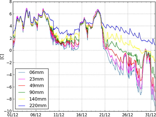
In Fig. 1, the 2 m temperature, snowfall and wind speed are depicted from 11 December 1996 until 30 January 1997. The 2 m temperature is below zero from 20 December until 12 January, apart from a small thawing event on 30 December 1996. In Fig. 2, the water temperature records are given and prior to the ice period there is an interesting feature. From 9 to 16 December, the air temperature is close to zero degrees and the water temperature profile becomes stratified. The warmest water is at the lowest level of 220 mm and the coldest water is just underneath the surface at 6 mm. Note that no ice has formed yet. On 16 December, the water column becomes more mixed due to higher air temperatures and higher wind speeds. The water column is not stratified anymore and the warmest water is now at the surface.

Fig. 1 Time series of 2 m temperature, snowfall and wind speed during the winter of 1996–1997 at Cabauw. The snowfall on 29 December 1996 is converted to a snow layer of 0.05 m.

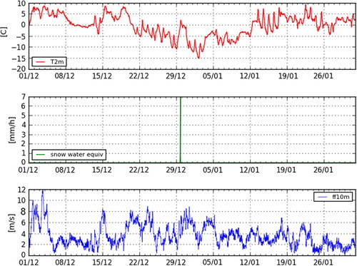
Fig. 2 Water temperature records at fixed depths from the surface at Cabauw (The Netherlands) during December 1996.

In Fig. 3, water temperatures from FLake and BW88 in this shallow ditch are presented. We show the bottom temperature (), the column temperature () and the temperature of the mixed layer () of FLake. From BW88 the column temperature () can only be shown. The models have some bias but represent the gross features rather well, but they cannot capture the details in the evolution of the water temperature profile. Note that the ditch is a shallow basin and possibly due the limited dimensions FLake is not able to adequately develop a complete system of a mixed and stable layer. When we look at the resulting ice thickness by the different models and the observations, as depicted in Fig. 4, we see that on 21 December the 2 m temperature drops below zero and ice is immediately formed. In the beginning, the ice-growth is fastest, because freezing energy is transported over a small layer. In a thicker ice layer, the growth levels off, because the freezing energy release at the ice–water interface is transported over a thicker ice layer. This gives rise to a roughly dependence of ice thickness on time (de Bruin and Wessels, 1988; Yang et al. 2012).

Fig. 3 Simulated water temperatures from FLake and BW88 during December 1996, Θ _s is mixed layer temperature, Θ _c is column temperature, Θ _b is bottom temperature, Θ_oper is the column temperature of BW88.

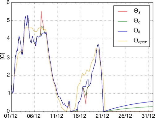
Fig. 4 Observed and simulated ice thickness at Cabauw during the winter of 1996–1997. The biases for FLake and BW88 are −0.0072 and −0.0067 m, respectively. Note that the lake models are driven by observations.

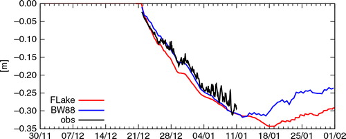
On 30 December, the temperature rises for a short while above the freezing level and snowfall is also reported. As a result, a levelling-off in the ice-growth can be recognised in both ice models. On 11 January, the thaw sets in and the ice layer starts to melt off. In this period, we cannot use the measured temperatures anymore for estimating the ice thickness, because the stratification has vanished and the profile becomes isothermal.

In the studied period, the biases for both lake models change sign, resulting in small values of −0.0072 and −0.0067 m for FLake and BW88, respectively. The RMSE-scores are an order of magnitude bigger, namely 0.015 and 0.014 m. BW88 has slightly better scores than FLake, but it should be noted that the dataset is rather small and it is doubtful if the scores are significant.

The BW88 model produces only a column averaged water temperature and cannot represent small-scale variations in time and in depth of the water temperature profile. FLake gives more details, but even the representation in two layers is not sufficient to capture all details. However, ice- and snow thickness, being variables with a longer time-scale, are quite well represented by both models. The timing of the onset of the ice floor is well captured by both lake ice models.

4.2. Regional ice predictions using HARMONIE input data

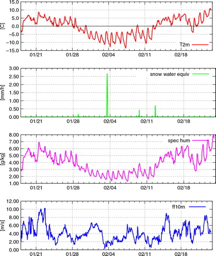
In this experiment, we use HARMONIE data to provide localised weather data. Instead of a ditch in Cabauw, our experiment is now located in the province of Friesland where there is a network of lakes and canals. To get rid of imbalances after the initialisation of the lake models, we allow a start-up period of 10 d. Figure 5 shows HARMONIE output for the city of IJlst. The frost period from 28 January to 12 February can be clearly recognised in the time series of the 2m temperature on the top panel. The synoptic situation had an anti-cyclonic character, resulting in a small cloud cover, and in a relatively small long-wave radiation flux from the atmosphere. Note that the BW88 model still uses the empirical formulas (1) and (2).

Fig. 5 2 m temperature, snowfall, specific humidity and 10 m wind simulated by HARMONIE for IJlst during the cold spell in January–February 2012.

The ice-growth in two locations in the province of Friesland, namely IJlst and Sloten show remarkable differences. At IJlst, a sheltered waterway with a limited fetch, the onset of ice-growth is well captured by the records from the voluntary observers, and noticeably earlier than at Sloten, which is located in the centre of a lake, compare Figs. 6 and 7. It is obvious that the wind delayed the freeze-up at Sloten, because it is a larger basin where mixing is an issue. This seems to be confirmed by some nearby observations.

Fig. 6 Modelled ice (top) and snow (bottom) thickness and observations for IJlst during January–February 2012.

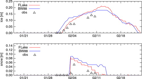
Fig. 7 Modelled ice (top) and snow (bottom) thickness and observations for Sloten during January–February 2012. Note the retarded freezing.

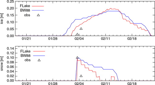
The onset of ice-growth in FLake is closer to the observations than BW88, at least in IJlst. In the BW88 model, the freeze-up is 3 d too early for both locations. In FLake, the onset is almost perfect in IJlst and 1 d early at Sloten. Flake benefits from the merits of the radiation scheme of HARMONIE, while BW88 applies relatively simple empirical formulas (1) and (2). In addition, FLake has a more advanced mixing scheme than the one-layer approach of the BW88 model and can better describe the evolution of the water temperature. Unfortunately, no observations of the melting period are available. Volunteers are reluctant to take their readings during this period, because they risk their wet suits.

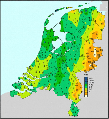
Another interesting feature during this episode is the snowfall, shown in Figs. 8 and 9 where 24-h accumulations are depicted for the HARMONIE model and observation stations in the Netherlands. It is clear that the snow pack is not evenly distributed and that the HARMONIE model reveals regional differences in the snow amounts. However, HARMONIE is not completely in accordance with the observations. There are areas where the snowfall is clearly over-predicted, for instance the area around the city of Dokkum where little snowfall is reported. Other locations in the middle of the Netherlands (Fig. 8) receive different snow amounts, which are confirmed by the observations.

Fig. 8 Predicted accumulated snowfall over 24 h valid on 4 February 2012 08 h UTC. Note the different snow amounts in Dokkum, IJlst, Sloten, Leersum, Loosdrecht and Cabauw.

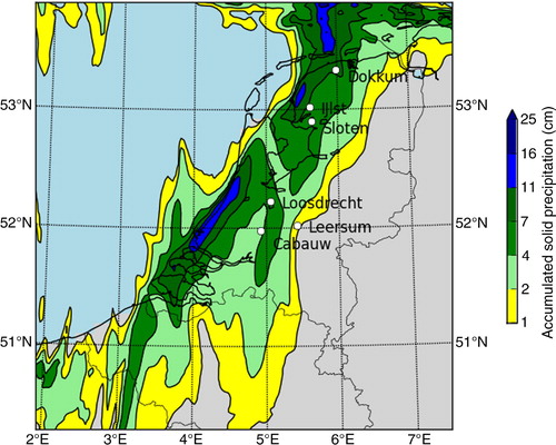
Fig. 9 Observed accumulated snowfall over 24 h valid on 4 February 2012 08 h UTC. Note that the snowfall is given in cm.

As soon as a relatively thin layer of ice is formed, it is covered by a snow layer. Both models capture this snow layer rather well, although the aging process is different. The snow layer slows down the process of ice formation, but in the end the ice thickness tends to be overestimated.

The timing of the break-up is modified by snow depth on the ice as well as by ice thickness and freshwater inflow. The freshwater inflow is mainly determined by the Dutch Water boards who are in charge of controlling the water level. During frost periods, pump stations suspend their water discharging task in order to encourage the ice-growth.

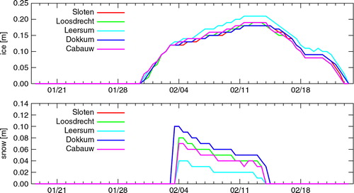
In Figs. 10 and 11, more regional forecasts of the lake models driven by HARMONIE data are depicted. Ice-growth was studied in five locations with a significantly different snow pack. These locations were Sloten, Loosdrecht, Leersum, Dokkum and Cabauw, which received different snow amounts (Fig. 8). In Fig. 10, the results of FLake are shown. In the beginning, the ice layer seems to grow according to a curve roughly proportional to . In Sloten and Leersum, the freeze-up date is 1 d later than at the other locations. For those locations, the ice-growth was slowed down by the snow pack. Leersum had less snow and this was favourable for the ice-growth. Dokkum received a fair amount of snow, but a reasonable layer of ice had already formed. This snow layer mainly impacted on the break-up date. With snow on the ice, the melting process is delayed. In Fig. 11, the results of BW88 are depicted and they show less regional differences. BW88 is a simpler model than FLake. Therefore, it cannot distinguish between the chosen water bodies in the Netherlands. Furthermore, the incoming radiation components are calculated with a relatively simple formulation.

Fig. 10 Modelled ice and snow thickness by FLake for five locations during January–February 2012.

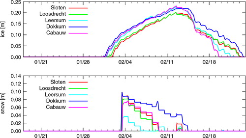
Fig. 11 Modelled ice and snow thickness by BW88 for five locations during January–February 2012.

5. Discussion

Here, we discuss the limitations of the applied lake parameterisations. In general, these parameterisations use a single column to model large inhomogeneous bodies of water, so clearly there are some representativity issues when choosing water depth, bottom temperature, fetch, etc.

Furthermore, fixed values for the extinction coefficients in water, ice and snow have been used. These parameters are based on measurements in Arctic regions. Perhaps these values have to be adopted for the Netherlands.

One feature that is neglected in this study is the conversion of snow to ice. Snow will get a higher density in the course of time. Moreover, it will melt and re-freeze again and eventually become part of the ice floor (Semmler et al., 2012; Yang et al. 2012). These processes have an impact on the ice thickness and they are not captured by BW88 or by FLake.

BW88 and FLake are 1D-models and account for interactions in the vertical only. Tendencies in the horizontal plane are not considered. For example, snow drift is not taken into account in HARMONIE or in FLake. This means that the distribution of snow is not affected by the wind, see (Lenaerts et al., 2012). Furthermore, no wind-induced currents in the lake are taken into account; the interaction of the wind drag to the ice floor is also not considered. Although the fetch is an input variable, it only affects the friction velocity for the exchange of momentum, heat and moisture fluxes.

6. Conclusions and outlook

FLake and BW88 cannot represent small-scale variations in the water profile in shallow basins, but ice- and snow-thickness, being variables with a longer timescale, are quite well represented and biases are smaller than 0.01 m. The BW88 model is a one-layer model and cannot describe a stratification. FLake is a two-layer model with more advanced physics and can represent a mixed layer. This leads to a better estimate of the onset of an ice layer on lakes. The timing error for FLake is less than 1 d, while BW88's timing error is more than 2 d.

The lake models in this study benefit from accurate atmospheric forcing provided by HARMONIE. Together with well-chosen set-up parameters (depth and fetch), local ice- and snow thicknesses can be produced. FLake reveals more variability in local ice- and snow thicknesses, because it is can distinguish between stable and unstable regimes. Moreover, it receives accurate radiation information from a state-of-the-art NWP model.

Lake models are sensitive to set-up parameters, suggesting the need to tune these parameters for specific bodies of water. Furthermore, lake models are sensitive to initial conditions and meteorological forcing data. Note that this sensitivity offers opportunities for ensembles techniques, which is a subject for further research.

Observations of ice thickness are sparse in the Netherlands. Therefore, it is difficult to validate and compare the lake models. Work is in progress to collect more data, also during the break-up period. Instead of manual observations, radar can also be applied to obtain ice thicknesses. First results with a penetrating ground based radar were promising. It is recommended to collect more ice thickness observations for model validation purposes and public safety.

7. Acknowledgments

Martin Stam and Rudolf van Westrhenen both from KNMI and many anonymous voluntary observers are thanked for collecting the observed data in the province of Friesland. Bert Heusinkveld and Adrie Jacobs of Wageningen University are acknowledged for their support in obtaining water temperatures at Cabauw. The positive criticism of three anonymous reviewers has improved the quality of this paper and the authors are grateful for their contributions.

References

- de Bruin H. A. R , Wessels H. R. A . A model for the formation and melting of ice on surface waters. J. Appl. Meteorol. 1988; 27: 164–173.
- FLake. Leibniz Institute of Freshwater Ecology and Inland fisheries. Leibniz Institute. http://www.flake.igb-berlin.de.
- Holtslag A. A. M , van Ulden A. P . A simple scheme for daytime estimates of surface fluxes from routine weather data. J. Clim. Appl. Meteorol. 1983; 22: 517–529.
- Launiainen J , Cheng B . Modelling of ice thermodynamics in natural water bodies. Cold Regions Sci. Tech. 1998; 27: 153–178.
- Lenaerts J. T. M , van den Broeke M. R , Déry S. J , van Meijgaard E , van de Berg W. J , co-authors . Regional climate modelling of drifting snow in Antarctica, Part I: Methods and model evaluation. J. Geophys. Res. 2012; 117: 1–17.
- Martynov A , Sushama L , Laprise R . Simulation of temperate freezing lakes by one-dimensional lake models: performance assessment for interactive coupling with regional climate models. Boreal. Environ. Res. 2010; 15: 143–164.
- Mironov D , Heisse E , Kourzeneva E , Ritter B , Schneider N , co-authors . Implementation of the lake parameterisation scheme FLake into numerical weather prediction model COSMO. Boreal. Environ. Res. 2010; 15: 218–230.
- Mironov D. V . Parameterization of lakes in numerical weather prediction. Description of a lake model. 2008. Technical report, Deutscher Wetterdienst, Offenbach am Main, Germany.
- Seity Y , Brousseau P , Malardel S , Hello G , Bénard P , co-authors . The AROME-France convective-scale operational model. Mon. Weather. Rev. 2011; 139: 976–991.
- Semmler T , Cheng B , Yang Y , Rontu L . Snow and ice on bear lake (Alaska) sensitivity experiments with two lake ice models. Tellus A. 2012; 64: 17339.
- Siebesma A. P , Soares P. M. M , Teixeira J . A combined Eddy-diffusivity mass-flux approach for the convective boundary layer. J. Atmos. Sci. 2007; 66: 1230–1248.
- Yang Y , Leppäranta M , Cheng B , Li Z . Numerical modelling of snow and ice thicknesses in Lake Vanajavesi, Finland. Tellus A. 2012; 64: 17202.