An operational analysis of Lake Surface Water Temperature

Abstract

Operational analyses of Lake Surface Water Temperature (LSWT) have many potential uses including improvement of numerical weather prediction (NWP) models on regional scales. In November 2011, LSWT was included in the Met Office Operational Sea Surface Temperature and Ice Analysis (OSTIA) product, for 248 lakes globally. The OSTIA analysis procedure, which has been optimised for oceans, has also been used for the lakes in this first version of the product. Infra-red satellite observations of lakes and in situ measurements are assimilated. The satellite observations are based on retrievals optimised for Sea Surface Temperature (SST) which, although they may introduce inaccuracies into the LSWT data, are currently the only near-real-time information available. The LSWT analysis has a global root mean square difference of 1.31 K and a mean difference of 0.65 K (including a cool skin effect of 0.2 K) compared to independent data from the ESA ARC-Lake project for a 3-month period (June to August 2009). It is demonstrated that the OSTIA LSWT is an improvement over the use of climatology to capture the day-to-day variation in global lake surface temperatures.

• LSWT
• OSTIA
• satellite
• in situ
• near-real-time

1. Introduction

Operational analyses of Lake Surface Water Temperature (LSWT) have many potential uses. Accurate estimates of LSWT have been shown to be of importance to numerical weather prediction (NWP) models on regional scales (e.g. Niziol et al., 1995; Dutra et al., 2010; Eerola et al., 2010; Mironov et al., 2010; Samuelsson et al., 2010; Balsamo et al., 2012; Wright et al., 2013) through their contribution to derived surface energy budgets. Maps of LSWT are also valuable for understanding a wide variety of processes occurring in lakes and inland water bodies, for example, surface water transport patterns (Strub and Powell, 1986, 1987; Steissberg et al., 2005b; Oesch et al., 2008), river inflow patterns (Thiemann and Schiller, 2003; Oesch et al., 2008), mixing regimes (Wooster et al., 2001), phytoplankton dynamics and primary production (Wooster et al., 2001; Thiemann and Schiller, 2003) and wind-induced upwelling events (Mortimer, 1952; Monismith, 1985, 1986; Imberger and Patterson, 1990; Steissberg et al., 2005a; Oesch et al., 2008). Surface temperature maps can provide information relevant to the vertical structure of the lake (Wooster et al., 2001) and can be useful for water quality monitoring (Reinart and Reinhold, 2008; Coats, 2010). Several studies have also used the surface temperature of lakes and inland water bodies as indicators of climate change, using both in situ observations (Quayle et al., 2002; Verburg et al., 2003; Coats et al., 2006) and infra-red satellite observations (Schneider et al., 2009; Schneider and Hook, 2010). Therefore accurate monitoring of LSWT has important applications.

The Operational Sea Surface Temperature and Ice Analysis (OSTIA) system (Donlon et al., 2012) was developed at the Met Office primarily for NWP purposes. The system produces a daily analysis of foundation Sea Surface Temperature (SST), the temperature below the diurnal warm layer, and sea ice concentration, on a global 1/20° grid. LSWT was included in OSTIA in November 2011 as part of the daily foundation SST field, at the same grid resolution. Prior to this, the Caspian Sea had been the only lake in OSTIA.

A description of the methods used to produce the OSTIA LSWT analysis follows in section 2. A review of the accuracy of satellite surface temperature retrievals over lakes is presented in section 3. In section 4, validation of the OSTIA LSWT analysis including a comparison to independent data from the ESA (European Space Agency) ATSR Reprocessing for Climate: Lake Surface Water Temperature and Ice Cover (ARC-Lake) project based at the University of Edinburgh (MacCallum and Merchant, 2011) for JJA (June to August) 2009 is discussed. In section 5, an examination of the relationships between accuracy of the LSWT analysis and parameters such as lake elevation and surface area is presented. Finally, a summary and conclusions are provided in section 6. Acronyms defined in the text have been listed in the appendix.

2. LSWT analysis method

A full description of the OSTIA system is provided in Donlon et al. (2012), but a brief introduction is included here for clarity. After quality control, near-real-time in situ data extracted from the Global Telecommunication System (GTS) and various near-real-time satellite SST data available through the Group for High Resolution SST (GHRSST) are assimilated daily on to a background field on a 1/20° (~6 km) grid, using an optimal-interpolation-type scheme. The background field is produced from the analysis for the preceding day, with a slight relaxation to climatology. New observations failing a Bayesian background check are rejected before assimilation (Donlon et al., 2012). Sea ice is produced by regridding the OSI SAF (EUMETSAT Ocean and Sea Ice Satellite Application Facility) near-real-time ice concentration product from a 10 km polar stereographic grid to the OSTIA regular latitude–longitude grid. This product is derived from the SSM/I (Special Sensor Microwave Imager) instrument, and more recently the SSMIS (Special Sensor Microwave Imager/Sounder). Bilinear interpolation is used to infill the pole hole and around coasts. Under sea ice, SSTs are relaxed to −1.8°C on a timescale which decreases with increasing ice concentration, as described in Donlon et al. (2012).

Many lakes are ice-covered for part of the year. Lake ice is added to the OSTIA ice field using a combination of NCEP (National Centers for Environmental Prediction) SSM/I ice concentration and a temperature threshold based on the LSWT analysis itself. OSTIA LSWT is relaxed towards the freezing temperature of fresh water (0°C) under the NCEP ice using the same method as for the SST. When available, SST observations from the AATSR (Advanced Along Track Scanning Radiometer) instrument or, more recently, a high-quality subset of MetOp-A AVHRR (Advanced Very High Resolution Radiometer) observations, together with in situ observations from ships, moored buoys and drifting buoys are used as reference data for bias-correction of the remaining satellite data. Observation error information provided in the GHRSST files is used for the analysis. In order to produce an analysis of foundation temperature, daytime satellite data are only assimilated where wind speeds are greater than 6 m s⁻¹ to remove surface diurnal warming effects (Donlon et al., 2002). This check is also performed for the LSWT data, as a skin effect of a similar magnitude and variability to that seen in oceans (e.g. Katsaros, 1977; Fairall et al., 1996; Donlon and Robinson, 1998) can also be observed in lakes (Wooster et al., 2001; Hook et al., 2003; Oesch et al., 2005, 2008).

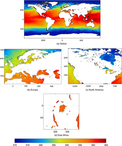
In the new implementation of OSTIA including lakes, the land/lake mask used is that defined by the ESA ARC-Lake project (MacCallum and Merchant, 2011). The full mask includes all lakes with a surface area greater than 500 km², plus an additional 10 lakes of particular interest, giving a total of 263 lakes. However, only 248 lakes have enough data to produce a climatology, so 248 lakes of the full 263 are included in OSTIA (see Fiedler et al., 2012 for full list). Figure 1 shows an example of the global OSTIA mask including lakes, with close-ups of Europe, North America and Eastern Africa for detail. As the mask is fixed, it is not possible for the OSTIA LSWT to take into account ephemeral lakes, rivers or regions of flooding.

Fig. 1 Example OSTIA SST field for 1 July 2013 showing (a) global land/sea/lake mask with (b–d) close-ups of regions for detail. Colourbar in K.

The ARC-Lake nighttime reconstructed AATSR climatology v1.1 (MacCallum and Merchant, 2011) has been used for lakes in the relaxation to climatology step when updating the background field during the OSTIA assimilation procedure, and for comparisons to climatology in the following sections. The climatology is on the same regular 1/20° grid as OSTIA. A linear temporal interpolation was performed on the ARC-Lake data to produce daily files from the original twice-monthly dataset available at the time of this investigation.

LSWT data are routinely available as part of GHRSST SST products for several of the infra-red satellite instrument sources used in OSTIA [AATSR, National Oceanic and Atmospheric Administration (NOAA) and MetOp-A AVHRR, Infrared Atmospheric Sounding Interferometer (IASI)]. However, none of these products currently includes lake-specific processing. Therefore the LSWT data used in this study and for the daily operational OSTIA analysis are based on the current algorithms for SST retrieval. This introduces errors into the LSWTs, which are described in detail in section 3. In situ data from ships and moored buoys are available for lakes through the GTS in the same way as in situ SST measurements.

The OSTIA analysis method has not been optimised for lakes and hence LSWT is currently produced in the same way as SST. This means the components of the analysis, such as background error covariances, are not specific to lakes. Effective correlation length scales in OSTIA range from 15 to 450 km, which means that if lakes are close enough to the ocean coast, increments applied over the ocean can also affect lakes. These length scales are also potentially long compared to a minimum lake area of 500 km², so increments applied in one lake can also be spread to a neighbouring lake, or an increment may be spread over a lake even if the observed part of the lake is atypical. However, use of this method does provide a starting point for future development work. In addition, AATSR and IASI skin temperature observations over lakes are corrected to bulk temperatures by applying a global correction of +0.17 K (Donlon et al., 2002) in the same way as is currently performed for SST in the OSTIA system. However, it is possible the magnitude of this correction may not be suitable for lakes, owing to the potentially different wind regimes compared to the open ocean.

Although there are many different satellite data types used in OSTIA (Donlon et al., 2012), comparisons and analyses for the OSTIA data are shown here for only the data types which provide lake ‘SSTs’ for the test period of JJA 2009. These are namely data from the NOAA-18 AVHRR, MetOp-A AVHRR and AATSR instruments. No LSWT data from microwave instruments were available. In improvements to OSTIA made for an operational change in November 2011, additional lake temperature data from IASI and NOAA-19 AVHRR also became available, but these data sources were not available for the test period. Note also that the AATSR instrument ceased production of data in April 2012.

3. Accuracy of LSWT retrievals

There will be errors in GHRSST LSWT satellite observations used in this study as retrievals are optimised for SST. This in turn introduces inaccuracies in the LSWT analyses using the data. Errors owing to the use of cloud-clearing schemes optimised for oceans can have a significant effect on the accuracy of retrievals over lakes (MacCallum and Merchant, 2012). There will also be errors associated with the elevation and continental location of the lakes, which affect the atmospheric thickness, water vapour column and aerosol corrections in the retrievals (Wooster et al., 2001; Thiemann and Schiller, 2003; MacCallum and Merchant, 2012). Coastal contamination is also a potential issue, particularly for lakes with complex shorelines, as are errors associated with surface emissivity, which is salinity dependent (MacCallum and Merchant, 2012). Errors in this latter quantity can lead to large errors in the derived surface temperature (Hook et al., 2003). Sparse observations and subsequent sampling errors are likely to particularly affect analyses for lakes in cloudy regions, or those for smaller lakes, especially when using satellite instruments with a narrow swath width such as the AATSR. Therefore the number of available observations may show considerable variation between even nearby lakes. In addition, sparse observations over lakes with large horizontal temperature gradients mean the observations may not be spatially representative of temperatures over the whole lake. However, although not ideal, the use of these SST retrievals over lakes is currently the only option for producing global near-real-time analyses of LSWT and brings the Met Office product into line with other SST analysis products, for example, the RTG_SST (Real Time Global Sea Surface Temperature) analysis produced by NCEP (Gemmill et al., 2007).

Several studies have attempted to quantify the errors introduced into LSWT retrievals when using parameters optimised for SST. Table 1 summarises the results of these studies for particular lakes. Nighttime results are shown where possible as they are likely to be significantly more accurate than those obtained during the daytime, owing to the absence of differential surface heating (Hook et al., 2003; Oesch et al., 2005). Note this effect is corrected for in the OSTIA system by using daytime data only when the wind speed is above 6 m s⁻¹.

Table 1. Accuracy of operational SST algorithms when used for LSWT

Instrument	Algorithm	Lake	Day/night	Bias (K)	RMS (K)	Study
NOAA-12 AVHRR	NLSST	N. Am. Great Lakes	Night	1.52	1.27 (SD)	2001)
NOAA-14 AVHRR	MCSST	Lake Constance	Day	1.35	1.35	2003)
NLSST	N. Am. Great Lakes	Night	0.41	0.80 (SD)	2001)
NOAA-16 AVHRR	MCSST	Lake Geneva	Night	0.18	0.70	2005)
Lake Constance	Night	−0.28	0.73	2005)
Lake Mond	Night	−2.08	1.47	2005)
NLSST	Lake Geneva	Night	1.22	0.69	2005)
Lake Constance	Night	0.61	0.64	2005)
Lake Mond	Night	−1.15	1.34	2005)
NOAA-17 AVHRR	MCSST	Lake Geneva	Night	0.70	0.88	2005)
Lake Constance	Night	−0.04	1.12	2005)
Lake Mond	Night	−2.03	1.83	2005)
NLSST	Lake Geneva	Night	1.53	0.81	2005)
Lake Constance	Night	0.85	1.12	2005)
Lake Mond	Night	−1.10	1.91	2005)
MetOp-A AVHRR	Operational	N. Am. Great Lakes	Night	0.06	0.50 (SD)	A. Marsouin (personal communication, 2009)
ATSR-2	Operational	Various N America, Europe, Africa	Night	−0.23–0.60	0.47–0.64 (SD)	MacCallum and Merchant (2012)
Lake Tahoe	Night	0.69	0.38 (SD)	2003)
AATSR	Operational	Various N America, Europe	Night	−0.54–0.08	0.83–1.74 (SD)	MacCallum and Merchant (2012)
Lake Tahoe	Night	−0.41	0.56	Hulley et al. (2011)
Salton Sea	Day	−0.41	0.75	Hulley et al. (2011)

SD=standard deviation. Instrument and algorithm acronyms defined in the appendix.

Results for Lake Mond are the poorest, but with a surface area of only 14 km² (Oesch et al., 2005) this lake is much smaller than the others shown in Table 1. It is much more difficult to produce an accurate result for a lake of this size because of sparse observations and coastal contamination. Owing to its small size, this lake is not included in the OSTIA mask (section 2). Results shown in Table 1 for MetOp-A AVHRR (used in OSTIA) for the North American Great Lakes are particularly good, with a bias of 0.06 K and root mean square (RMS) error of 0.50 K against in situ temperatures from moored buoys (A. Marsouin, personal communication, 2009). For the NOAA-17 AVHRR MCSST (Multi-Channel Sea Surface Temperature) algorithm (closest to the operational NOAA-18 AVHRR MCSST used in OSTIA) the biases for Lakes Constance and Geneva, respectively, are −0.04 and 0.70 K with RMS errors of 0.88 and 1.12 K. Both of these lakes have similar size, elevation and location characteristics. However, the RMS error and bias of the data obtained vary widely depending on the chosen lake, and this illustrates the difficulty in assessing the accuracy of the use of these algorithms over lakes. Overall, however, biases for instruments used in OSTIA (MetOp-A and NOAA AVHRR, AATSR) are mainly of the order 0.5 K and RMS errors around 1.0 K (Table 1).

Several other studies have evaluated LSWT algorithms designed for specific lakes (Hook et al., 2003; Thiemann and Schiller, 2003; Oesch et al., 2008). More recently, these have been expanded to include larger numbers of lakes (Hulley et al., 2011; MacCallum and Merchant, 2012). Details of these results are given in Table 2. According to Thiemann and Schiller (2003), it should be suitable to apply regional algorithms derived for specific lakes to other lakes with similar climatic conditions, for example, temperate or maritime/continental. However, a lower absolute accuracy compared to open ocean retrievals is to be expected for lake-specific retrievals owing to the reduced spatial and temporal coverage over lakes (Oesch et al., 2005).

Table 2. Accuracy of LSWT algorithms designed for lakes

Instrument	Algorithm	Lake	Day/night	Bias (K)	RMS (K)	Study
NOAA-11 AVHRR	Split window	Lake Malawi	Night	−0.02	0.68	2001)
Triple window	Lake Malawi	Night	−0.17	0.41	2001)
NOAA-14 AVHRR	Split window	Lake Constance	Day	−0.01	1.04	2003)
Triple window	Lake Malawi	Night	0.06	0.51	2001)
NOAA-16 AVHRR	Split window	Lake Constance	Day	0.16	0.71	2003)
ATSR-2	ARC-Lake OE (N2,N3,D2,D3)	Various N America, Europe, Africa	Night	−0.04–0.04	0.53–0.61 (SD)	MacCallum and Merchant (2012)
N2,N3 (bulk)	Lake Tahoe	Night	0.18	0.18 (SE)	2003)
N2,N3 (skin)	Lake Tahoe	Night	−0.37	0.28 (SE)	2003)
AATSR	Split window	Lake Tahoe	Night	−0.02	0.30	Hulley et al. (2011)
Split window	Salton Sea	Day	0.18	0.46	Hulley et al. (2011)
ARC-Lake OE (N2,N3,D2,D3)	various N America, Europe	Night	−0.31–0.15	0.46–0.54 (SD)	MacCallum and Merchant (2012)
ARC-Lake OE LSWT (D3)	N. Am. Great Lakes	Night	−0.12	0.43 (SD)	MacCallum and Merchant (2012)

Nx=Nadir channel x; Dx=dual view channel x; SD=standard deviation; SE=standard error. Instrument acronyms defined in the appendix.

There are other studies relating to satellite-derived LSWT from other sensors, for example, MODIS (Moderate Resolution Imaging Spectroradiometer) (Oesch et al., 2005, 2008; Reinart and Reinhold, 2008; Crosman and Horel, 2009), but sensors not currently used in OSTIA have not been covered here. Results for older AVHRR sensors on NOAA satellites (NOAA-11 and earlier) have also not been included. Currently, there are no GHRSST microwave satellite SST retrievals which include LSWT.

4. Validation of OSTIA LSWT analysis

OSTIA LSWT daily analysis data were produced for JJA 2009. This period was chosen in order to make use of the ARC-Lake observation dataset (MacCallum and Merchant, 2011) for validation, of which 2009 was the most recent year available, at the time of writing. As the majority of the lakes in the OSTIA mask are located in the Northern Hemisphere (Fig. 1), JJA corresponds predominantly to summertime. It should be noted there is only one lake included in the OSTIA mask which freezes in the Southern Hemisphere wintertime (JJA), which is Colhue Huapi, Argentina (69°W, 45°S). In contrast, up to 100 lakes freeze in the Northern Hemisphere wintertime (MacCallum and Merchant, 2011). It is not possible to provide a fair quality assessment of the OSTIA LSWT in DJF owing to the limited number of observations available for assimilation when there is ice cover, which would make results unrepresentative of errors expected in the OSTIA LSWT analysis. The OSTIA run was given a generous 6-month spin-up period, allowing the analysis to depart from the ARC-Lake climatology it was initialised with, taking into account that observations over lakes can be sporadic owing to satellite orbits and cloud cover.

4.1. Number of observations

The number of available infra-red satellite observations is affected by cloud cover, meaning there are large day-to-day variations in the volume of data. This is illustrated in Fig. 2. Of the satellite LSWT data sources, the MetOp-A AVHRR has the largest data volume (compare Fig. 2c to Fig. 2a and 2b). This is the highest resolution data source, at 6 km (after subsampling of 1 km resolution data). In contrast, the narrow swath width of the AATSR instrument means it takes just over 3 days to achieve complete global coverage (Robinson, 2004) and thus the number of observations over lakes can be sparse and very variable from day to day (Fig. 2a).

Fig. 2 Total daily number of observations by instrument type for all lakes in OSTIA mask, for JJA 2009.

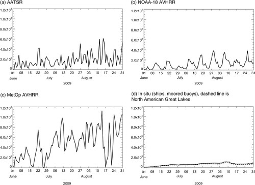
Comparison of the global number of in situ observations with that for the North American Great Lakes (Fig. 2d) indicates the majority (3-month mean of 83%) are located on the Great Lakes. The bias-correction method for the OSTIA LSWT, as for the SST, uses the in situ data and AATSR data together as a reference dataset. Thus for most of the lakes the only reference data used for the bias-correction is the AATSR, which is not optimised for lakes. Retrieval methods for LSWT suitable for the ATSR series of instruments (ATSR-1, ATSR-2 and AATSR) are available through the ARC-Lake project (MacCallum and Merchant, 2012) but, as they do not form part of the operational processing chain, cannot be used in near-real-time.

4.2. Observation-minus-background statistics

Table 3 shows the observation-minus-background statistics (i.e. before the observations are assimilated or bias-corrected) for OSTIA LSWT for JJA 2009 globally and for three lake system case studies: Lake Victoria (centred on 33°E, 2°S), Lake Baikal (centred on 108°E, 53°N) and the North American Great Lakes (centred on 85°W, 46°N). For each data type, the observations for a particular day are compared against a background field of the analysis for the previous day. If the observations are assumed to be accurate, this comparison gives a measure of the accuracy of the analysis. Although the errors in the observations are not independent from the errors in the analysis, on comparison to results using independent data this method still provides useful results (e.g. Roberts-Jones et al., 2011). The daily results are averaged over the 3-month period to give the seasonal results shown in Table 3.

Table 3. Observation-minus-background statistics for JJA 2009, for all lakes in global OSTIA mask and three case studies

Observation type	Mean diff (K)	RMS (K)	Mean daily no. obs
Global
In situ	−0.13	1.02	600
AATSR	0.08	0.83	1826
MetOp-A AVHRR	0.20	1.12	4740
NOAA-18 AVHRR	−0.08	0.49	1153
Great Lakes
In situ	−0.14	1.01	498
AATSR	0.13	0.97	447
MetOp-A AVHRR	0.46	1.29	1699
NOAA-18 AVHRR	−0.06	0.55	230
Lake Baikal
In situ	−	−	−
AATSR	0.49	1.20	35
MetOp-A AVHRR	0.42	1.65	159
NOAA-18 AVHRR	0.59	1.14	7
Lake Victoria
In situ	−	−	−
AATSR	0.07	0.32	193
MetOp-A AVHRR	0.06	0.44	621
NOAA-18 AVHRR	−0.14	0.30	206

A dash (−) indicates no or insufficient data.

Overall, the statistics given by Table 3 are encouraging. The global RMS difference of the OSTIA LSWT to in situ data is 1.02 K and the mean difference is −0.13 K. These global statistics are similar to those shown for the Great Lakes (Table 3), which is unsurprising since the majority of the in situ data for this period (83%) are located in this lake system.

Compared to the Great Lakes and Lake Victoria, Lake Baikal has the largest mean and RMS difference for most of the satellite data types (Table 3). This could be related to, for example, cloud screening errors. The exception is the mean difference to MetOp-A AVHRR, which is marginally worse in the Great Lakes (0.42 K for Lake Baikal, 0.46 K for the Great Lakes). The magnitude of this relatively large mean difference for the Great Lakes is an interesting result, given the bias of MetOp-A AVHRR shown in Table 1 of 0.06 K on comparison to in situ moored buoys (A. Marsouin, personal communication, 2009). Comparing the two AVHRR data sources, Table 3 indicates the RMS difference of the observation-minus-background for the NOAA-18 AVHRR is smaller than for the MetOp-A AVHRR for each of the lakes shown. The magnitude of the mean difference to NOAA-18 AVHRR is also smaller globally and for the Great Lakes than for MetOp-A AVHRR, but is slightly larger for Lakes Baikal and Victoria. Overall, Lake Victoria has smaller mean and RMS differences compared to the other lakes. Its position on the equator, modest elevation and large size mean a more accurate LSWT analysis should be possible. Reasons for variations in the accuracy of the LSWT analysis are discussed further in the following sections.

4.3. Comparison to independent data

The ARC-Lake LSWT retrievals employ a cloud screening scheme designed for lakes and a modelled emissivity, and take into account the elevation of the lakes and the atmospheric conditions above them (MacCallum and Merchant, 2012). This not only means the observations are independent from the AATSR data assimilated into OSTIA, which uses the operational SST algorithm, but that they can be considered the most reliable global satellite observations of LSWT available. In the absence of observations, OSTIA will relax to a climatology generated from ARC-Lake observations, over a 30-day time period. In practice, this means the OSTIA LSWT is climatology in wintertime, if new observations are unavailable due to ice cover. However, at other times of the year the number of available observations over a 30-day period ensures the LSWT remains independent from the climatology, including for the JJA 2009 period used here. Therefore a validation of the OSTIA LSWT against the ARC-Lake observation dataset was undertaken. It should however be noted the ARC-Lake observations are measurements of skin temperature, whereas the OSTIA analysis is a foundation temperature. Nighttime ARC-Lake observations have been used in the comparison to avoid the effects of diurnal warming, but a cool skin effect of around 0.2 K is present (MacCallum and Merchant, 2012). Note this has not been removed from the results.

Globally, the accuracy of the OSTIA LSWT against the ARC-Lake observations is 1.31 K RMS (Table 4). At 0.65 K, the magnitude of the mean difference indicates that using AATSR processed for SST and limited in situ data for the bias-correction is not ideal. However, the cool skin effect mentioned above means this mean difference can be assumed closer to 0.45 K. The global statistics given in Table 4 indicate that the RMS difference for OSTIA minus ARC-Lake observations (1.31 K) is better (lower) than for ARC-Lake climatology minus ARC-Lake observations (1.78 K), demonstrating that overall the OSTIA LSWT is more accurate than climatology. Since the ARC-Lake climatology is derived from ARC-Lake observations, the mean difference of the climatology to these observations would be expected to be smaller than for OSTIA and indeed is zero when taking all lakes together globally (Table 4).

Table 4. OSTIA LSWT minus ARC-Lake observations and ARC-Lake climatology minus ARC-Lake observations for JJA 2009 for selected lakes, listed in order of descending surface area

OSTIA-ARCobs		ARCclim-ARCobs
Observation type	Mean diff (K)	RMS (K)	Mean diff (K)	RMS (K)	Mean daily no. ARCobs
Global	0.65	1.31	0.00	1.78	4453
Great Lakes	1.41	1.78	0.45	2.13	822
Lake Victoria	0.40	0.44	0.08	0.29	137
Lake Baikal	1.83	2.76	1.21	2.11	140
Salton Sea	−0.13	1.45	−0.15	1.44	7
Lake Geneva	−0.06	0.63	1.00	1.67	2
Lake Constance	−0.06	1.02	0.95	1.87	1
Lake Tahoe	−0.46	0.83	0.28	0.82	2

Case studies of particular lakes are also shown in Table 4. The OSTIA LSWT analyses for both the Great Lakes and Lake Baikal have large mean and RMS differences compared to the other lakes and, in the case of Lake Baikal, the analysis performs worse than the climatology in terms of the RMS. However, results for other lakes are relatively good, particularly for Lakes Geneva and Constance. The magnitudes of the OSTIA minus ARC-Lake observation mean and RMS differences are generally larger than the observation-minus-background errors discussed previously in section 4.2; compare Table and 4 .

Comparison of Table 4 (OSTIA LSWT accuracy) with Table 1 (SST retrieval accuracy) yields mixed results. For Lakes Geneva and Constance, compared to the results of Oesch et al. (2005) using the NOAA-17 AVHRR MCSST algorithm (the closest to the assimilated NOAA-18 data), the OSTIA LSWT RMS errors are reduced and the mean differences are similar or better. For Lake Tahoe, compared to results from Hulley et al. (2011) using the AATSR SST data, the magnitude of the mean difference is similar but the RMS difference is worse for the OSTIA data compared to the operational AATSR retrievals. Similarly, the results for the Salton Sea show an improved mean difference for the OSTIA data but a poorer RMS. For the Great Lakes, the OSTIA results are poorer than those found for both the MetOp-A AVHRR and the AATSR operational retrievals. This indicates the OSTIA LSWT results for the Great Lakes are worse than the individual retrievals. This could potentially be due to poor quality in situ data used in the analysis for bias-correction. The in situ data used in this assimilation have not undergone the usual operational monthly check against OSTIA data for potential inclusion on a blacklist. In addition, the majority of these data come from ships which can provide data of reduced quality than those obtained from moored (or drifting) buoys (Roberts-Jones et al., 2012). As the analysis appears to provide poorer results than the individual retrievals, this could indicate the analysis techniques, which are currently optimised for SST, need improving. It could also suggest that the accuracy of the retrievals summarised in Table 1 may not be consistently as good as the published results suggest, for example, due to cloud screening errors. Comparison of Table 4 (OSTIA LSWT accuracy) with Table 2 (LSWT retrieval accuracy) indicates the OSTIA LSWT analysis is not as accurate and has greater biases than LSWTs obtained from lake-specific non-operational LSWT retrieval algorithms, which is to be expected.

The target accuracy of the OSTIA analysis for NWP purposes is at or below 0.50 K RMS with a threshold accuracy of 0.80 K (Donlon et al., 2012). At 1.31 K against independent ARC-Lake observations, the global RMS difference of the OSTIA LSWT analysis does not meet this requirement. However, it has been demonstrated here that use of the analysis would nevertheless be an improvement over the use of climatology. As would be expected, owing to the use of retrieval algorithms and analysis techniques optimised for SST rather than LSWT (section 2), the accuracy of the OSTIA LSWT analysis is poorer than for the SST [respectively, global RMS differences of 1.31 K (for JJA 2009) and 0.57 K (for 2007–2010, in situ observation-minus-background) (Donlon et al., 2012)].

5. Investigation of relationships between analysis accuracy and lake parameters

Various metadata for each lake in the mask have been collated by the ARC-Lake project (MacCallum and Merchant, 2011). This section describes investigations of the relationships between the accuracy of the OSTIA LSWT analysis as measured by differences from the ARC-Lake observations (section 4.3), and parameters including the elevation, area, and latitude of the lakes.

Figure 3 shows the OSTIA LSWT analysis minus ARC-Lake nighttime observations, averaged over JJA 2009, plotted as a function of absolute latitude (i.e. disregarding hemisphere). Each point represents a lake, where a red triangle is a lake at an elevation above 2500 m and a black dot indicates an elevation at or below 2500 m. A blue square indicates the lake also has an area larger than 3000 km².

Fig. 3 OSTIA LSWT analysis minus ARC-Lake observations for each lake, for JJA 2009, with absolute latitude (i.e. disregarding hemisphere) with (a) RMS and (b) mean difference. Each point represents a lake. A red triangle indicates the lake has an elevation over 2500 m, and a black dot equal to or below 2500 m. A blue square indicates the lake also has a surface area of greater than 3000 km².

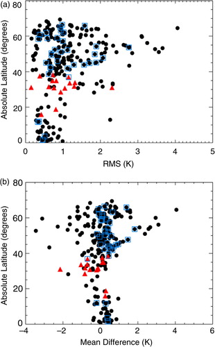
As would be expected, the difference between the mean difference of the analysis and ARC-Lake observations for the two hemispheres is not statistically significant (not shown). Lakes at tropical latitudes have a smaller annual surface temperature cycle compared to lakes at higher latitudes (MacCallum and Merchant, 2012), which suggests it would be easier to obtain smaller RMS values for lower latitude lakes in a LSWT analysis. Indeed, there is a statistically significant difference (at the 0.05 level) between the RMS difference of lakes with latitudes above 30° (1.41 K) and those below 30° (0.74 K) in the summer season (JJA) (Fig. 3a). This statistic (and subsequent similar statistics) was calculated using Welch's t-test for unequal sample sizes and variances, and the Welch-Satterthwaite equation for calculating degrees of freedom. The significances are all given at the 0.05 level. This method assumes the two samples are independent (non-paired), although this may not be strictly true here as the errors may be correlated. Unlike the RMS values, however, the mean difference to ARC-Lake observations for these two groups is not statistically significantly different, indicating that latitude is not a contributing factor to biases in the LSWT analysis.

There is not a strong relationship between the magnitude of the mean difference to ARC-Lake and the lake area (Fig. 3b), although smaller lakes are more likely to have a larger mean difference, and the largest lakes are more likely to have a mean difference closer to zero. Most of the lakes shown here have a minimum area of 500 km² so it is possible an effect of area on bias would become more apparent for smaller lakes. As demonstrated by Oesch et al. (2005) for Lake Mond (see Table 1), very small lakes can display large biases.

Figure 3b also indicates that lakes at high elevations are more likely to have a negative mean difference to ARC-Lake, although lakes at low elevations can also have a negative mean difference. The JJA 2009 mean of the difference to ARC-Lake for all lakes lying above 2500 m elevation (−0.37 K) is statistically significantly different to that of lakes below 2500 m (0.12 K). As noted by, for example, Schneider and Hook (2010), large lakes at modest elevations might be expected to provide the best results for LSWT using the SST products. According to Fig. 3b, these lakes have a positive bias. This means that the LSWT for higher altitude, smaller lakes may have compensating errors, thus reducing the bias. As indicated by the global OSTIA LSWT minus ARC-Lake observations statistics (Table 4), overall the OSTIA LSWT has a positive mean difference.

There is little obvious relationship between RMS and lake area or elevation (Fig. 3a). In order to affect the accuracy of surface temperature retrievals, according to Oesch et al. (2005) the elevation would need to be extreme. In their study of Alpine LSWT, they did not find that the smaller atmospheric water vapour content at around 400 m elevation exerted a significant influence on the accuracy of the retrievals. According to Schneider et al. (2009), larger uncertainties in LSWT may be expected for lakes at more extreme elevations on the Tibetan Plateau and in the Andes although Fig. 3a (above 2500 m, red triangles) indicates this does not appear to be the case for the OSTIA data. However, other compensating errors may be masking an effect.

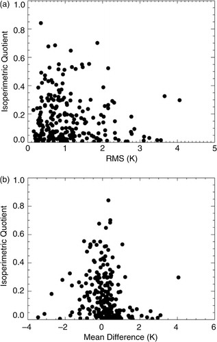
Figure 4 shows the RMS and mean differences to ARC-Lake of all OSTIA lakes for JJA 2009 versus the isoperimetric quotient. This metric involves the area of the lake divided by the square of the perimeter, and was calculated for lakes where these data were available. This ratio is multiplied by 4π, and the resultant value will be 1 if the shape is a perfect circle. When used in this context, the metric gives a measure of the regularity of the shape of the lake. Those lakes with less meandering shorelines will have an isoperimetric quotient closer to that of a circle; that is, the smallest perimeter possible for the area given. More accurate satellite measurements should be possible for lakes with an even perimeter and shorter coastline for a given lake area as this minimises potential contamination of the retrieval from land. It can be seen (Fig. 4a) that lakes with a higher quotient, that is, more circular and thus potentially likely to have more accurate retrievals, tend to have a lower RMS difference. Similarly, lakes with a higher quotient are more likely to have a smaller mean difference (Fig. 4b).

Fig. 4 OSTIA LSWT minus ARC-Lake observations for each lake, for JJA 2009, with isoperimetric quotient (a measure of how close to circular the lake is, or the regularity of the coastline, see text) with (a) RMS and (b) mean difference.

Figure 5 shows observation-minus-background statistics for in situ and AATSR observations before assimilation. These are averages for JJA 2009, shown with the elevation of each lake. Figure 5a shows that the bias-correction using the in situ data is working well, as the observation-minus-background bias for in situ data remains around zero for all elevations with the exception of a single outlier. This observation platform is located in Lake Ladoga (31°E, 61°N). In situ observations from this location are suspect as the data must be disagreeing with the rest of the observations assimilated into the analysis for this lake.

Fig. 5 Mean difference of (a) in situ observations minus OSTIA LSWT background and (b) AATSR observations minus OSTIA LSWT background. For each lake with available observations, for JJA 2009, with elevation. Note that 83% of in situ observations are located in the North American Great Lakes, whereas AATSR is spread globally.

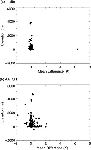
On comparison with Fig. 5a, the equivalent plot for the AATSR (Fig. 5b) shows more of a spread in the mean difference at various elevations, despite this also being used as a reference dataset. This may be related to the temporal sampling of the AATSR data, as there could potentially be several days or more between these measurements, allowing the LSWT analysis to drift away from the AATSR reference.

Similar plots for mean and RMS difference to ARC-Lake were examined for any relationships with lake depth and volume but none were found.

6. Summary and conclusions

Operational analyses of LSWT have many potential uses, including improvement of NWP models on regional scales. Therefore LSWT was included in the Met Office OSTIA product in November 2011 for 248 lakes globally. The OSTIA LSWT analysis is produced in the same way as the SST analysis using in situ data from the GTS where available and GHRSST satellite data. Not all satellite data types used in OSTIA contain LSWT information. AVHRR data from the MetOp-A and NOAA-18 satellites and AATSR data from Envisat were used for this study. There is significant day-to-day variation in the number of infra-red satellite surface temperature observations available over lakes because of cloud cover and the relatively small surface area to be captured in a satellite overpass. As the retrievals from the satellite instruments are optimised for SST, their use will introduce inaccuracies in a LSWT analysis, but these are currently the only data sources available for producing a near-real-time analysis. The OSTIA analysis procedure uses components designed for oceans for this first version of the LSWT product.

The global accuracy of the OSTIA LSWT product for JJA (June to August) 2009 compared against independent satellite observations from the ESA ARC-Lake project based at the University of Edinburgh (MacCallum and Merchant, 2011) is 1.31 K (RMS) with a mean difference of 0.65 K (OSTIA minus ARC-Lake, and including a cool skin effect of around 0.2 K). Using in situ observations, the global observation-minus-background statistics are 1.02 K (RMS) and −0.13 K (mean difference) for the same period, although most of these observations (83%) are located in the North American Great Lakes. The global accuracy of the OSTIA LSWT analysis is poorer than that of the operational SST analysis [0.57 K RMS (Donlon et al., 2012)] as would be expected. Although it does not meet the ideal accuracy requirement for NWP of 0.50 K RMS with a threshold of 0.80 K (Donlon et al., 2012), it has been demonstrated that the OSTIA LSWT is an improvement over the use of the ESA ARC-Lake climatology to capture the day-to-day variation in global lake temperatures.

There are clearly a number of factors which can potentially affect the accuracy of a LSWT analysis for an individual lake. It might be expected that LSWT analyses for large lakes at low altitudes, that is, those which approximate the oceans for which the retrievals and analysis methods are optimised, would produce the best results. This would also apply to those lakes with less complex shorelines, minimising the impact on the satellite retrievals from coastal contamination. It has been shown that analyses for lakes with all these qualities tend to have a positive bias, so it is possible that compensating errors in the analyses exist for smaller lakes at higher elevations, reducing the bias found for these lakes. It has also been demonstrated that analyses for lakes within 30° of the equator have smaller RMS differences. Using all these criteria, the three ‘best’ lakes in the OSTIA LSWT analysis are Lake Nyasa/Malawi (mean difference 0.30 K, RMS 0.33 K compared to ARC-Lake observations), Lake Tanganyika (mean difference 0.37 K, RMS 0.41 K) and Lake Victoria (mean difference 0.40 K, RMS 0.44 K). Note these lakes meet the target accuracy requirement for NWP of 0.50 K RMS mentioned above and certainly meet the threshold of 0.80 K. Each of these lakes also has an average of several hundred satellite observations per day for the test period of JJA 2009. Sampling issues are however clearly an important source of error for many lakes in the LSWT analysis as cloud cover and the frequency of satellite overpasses, as well as wintertime ice cover mean the number of observations can be sparse.

The magnitude of the bias in the OSTIA LSWT analysis compared to independent ARC-Lake satellite data (MacCallum and Merchant, 2011) indicates that the reference dataset used to estimate the bias-correction for the analysis could be improved. A near-real-time reference dataset with lake-specific processing, including improved retrievals and cloud-clearing schemes, is therefore likely to be of significant benefit to the quality of the OSTIA LSWT analysis.

Future work on the OSTIA LSWT analysis itself should also include verification of wintertime lake ice concentration and LSWT. In addition, the problem of sparse data over lakes means the analysis can drift towards climatology in the absence of observations, particularly in wintertime when ice cover prevents LSWT retrievals. An improved background check for quality control of observations over lakes would avoid the problem of rejecting good quality observations when the analysis drifts too far. This could be achieved by developing more suitable background errors for lakes and tuning the parameters specified a priori in the Bayesian background check. The use of lake-specific background error variances and correlation length scales would not only improve the analysis but also avoid spreading analysis increments too far. This issue could further be improved by, if necessary, preventing increments from being spread between lakes, or from the ocean to a lake.

7. Acknowledgements

We thank two anonymous reviewers for their helpful comments, and gratefully acknowledge the work of Stuart MacCallum and Chris Merchant on the ARC-Lake climatology, observations and metadata used in this paper.

8. Appendix

List of acronyms (A)ATSR – (Advanced) Along Track Scanning Radiometer

ARC-Lake – ATSR Reprocessing for Climate: Lake Surface Water Temperature and Ice Cover

AVHRR – Advanced Very High Resolution Radiometer

ESA – European Space Agency

GHRSST – Group for High Resolution Sea Surface Temperature

IASI – Infrared Atmospheric Sounding Interferometer

LSWT – Lake Surface Water Temperature

MCSST – Multi-Channel Sea Surface Temperature (algorithm)

NCEP – National Centers for Environmental Prediction

NLSST – Non-Linear Sea Surface Temperature (algorithm)

NOAA – National Oceanic and Atmospheric Administration

NWP – numerical weather prediction

OSI SAF – EUMETSAT Ocean and Sea Ice Satellite Application Facility

OSTIA – Operational Sea Surface Temperature and Ice Analysis

RMS – root mean square

SST – Sea Surface Temperature

SSM/I – Special Sensor Microwave Imager

SSMIS – Special Sensor Microwave Imager/Sounder

References

- Balsamo G. , Salgado R. , Dutra E. , Boussetta S. , Stockdale T. , co-authors . On the contribution of lakes in predicting near-surface temperature in a global weather forecasting model. Tellus A. 2012; 64: 15829. DOI: 10.3402/tellusa.v64i0.15829.
- Coats R . Climate change in the Tahoe basin: regional trends, impacts and drivers. Clim. Change. 2010; 102: 435–466.
- Coats R. , Perez-Losada J. , Schladow G. , Richards R. , Goldman C . The warming of Lake Tahoe. Clim. Change. 2006; 76: 121–148.
- Crosman E. T. , Horel J. D . MODIS-derived surface temperature of the Great Salt Lake. Rem. Sens. Environ. 2009; 113(1): 73–81.
- Donlon C. J. , Martin M. , Stark J. , Roberts-Jones J. , Fiedler E. , co-authors . The Operational Sea Surface Temperature and Sea Ice Analysis (OSTIA) system. Rem. Sens. Environ. 2012; 116: 140–158.
- Donlon C. J. , Minnett P. J. , Gentemann C. , Nightingale T. J. , Barton I. J. , co-authors . Toward improved validation of satellite sea surface skin temperature measurements for climate research. J. Clim. 2002; 15: 353–369.
- Donlon C. J. , Robinson I. S . Radiometric validation of ERS-1 along track scanning radiometer average sea surface temperature in the Atlantic Ocean. J. Atmos. Ocean. Technol. 1998; 15: 647–660.
- Dutra E. , Stepanenko V. M. , Balsamo G. , Viterbo P. , Miranda P. M. , co-authors . An offline study of the impact of lakes on the performance of the ECMWF surface scheme. Boreal Environ. Res. 2010; 15: 100–112.
- Eerola K. , Rontu L. , Kourzeneva E. , Shcherbak E . A study on effects of lake temperature and ice cover in HIRLAM. Boreal Environ. Res. 2010; 15: 130–142.
- Fairall C. W. , Bradley E. F. , Godfrey J. S. , Wick G. A. , Edson J. B. , co-authors . Cool-skin and warm-layer effects on sea surface temperature. J. Geophys. Res. 1996; 101C: 1295–1308.
- Fiedler E. K. , Martin M. , Roberts-Jones J . Lake Surface Water Temperature in the Operational OSTIA System. 2012; Met Office, Exeter, UK. Technical Report 565.
- Gemmill W. , Katz B. , Li X . Daily Real-Time, Global Sea Surface Temperature – High-Resolution Analysis RTG_SST_HR. 2007; NOAA, Camp Springs, MD. Office Note Marine Modeling and Analysis Branch, Contribution Number 260, Environmental Modeling Center, National Centers for Environmental Prediction, National Weather Service.
- Hook S. J. , Prata F. J. , Alley R. E. , Abtahi A. , Richards R. C. , co-authors . Retrieval of lake bulk and skin temperatures using Along-Track Scanning Radiometer (ATSR-2) data: a case study using Lake Tahoe, California. J. Atmos. Ocean. Technol. 2003; 20: 534–548.
- Hulley G. C. , Hook S. J. , Schneider P . Optimized split-window coefficients for deriving surface temperatures from inland water bodies. Rem. Sens. Environ. 2011; 115: 3758–3769.
- Imberger J. , Patterson J. C . Physical limnology. Adv. Appl. Mech. 1990; 27: 303–475.
- Katsaros K. B . Sea-surface temperature deviation at very low wind speeds – is there a limit?. Tellus. 1977; 29: 229–239.
- Li X. , Pichel W. , Clemente-Colón P. , Krasnopolsky V. , Sapper J . Validation of coastal sea and lake surface temperature measurements derived from NOAA/AVHRR data. Int. J. Rem. Sens. 2001; 22(7): 1285–1303.
- MacCallum S. N. , Merchant C. J . ARC-Lake v1.1, 1995–2009 [dataset]. 2011
- MacCallum S. N. , Merchant C. J . Surface water temperature observations of large lakes by optimal estimation. Can. J. Rem. Sens. 2012; 38(1): 25–45. DOI: 10.5589/m12–010.
- Mironov D. , Heise E. , Kourzeneva E. , Ritter B. , Schneider N. , co-authors . Implementation of the lake parameterisation scheme FLake into the numerical weather prediction model COSMO. Boreal Environ. Res. 2010; 15: 218–230.
- Monismith S. G . Wind-forced motion in stratified lakes and their effect on mixed-layer shear. Limnol. Oceanogr. 1985; 30: 771–783.
- Monismith S. G . An experimental study of the upwelling response of stratified reservoirs to surface shear stress. J. Fluid Mech. 1986; 171: 407–439.
- Mortimer C. H . Water movements in lakes during summer stratification: evidence from the distribution of temperature in Windermere. Philos. Trans. Roy. Soc. Lond. 1952; B236: 355–404.
- Niziol T. A. , Snyder W. R. , Waldstreicher J. S . Winter weather forecasting throughout the Eastern United States. Part IV: lake effect snow. Weather Forecast. 1995; 10: 61–77.
- Oesch D. C. , Jaquet J.-M. , Hauser A. , Wunderle S . Lake surface temperature retrieval using Advanced Very High Resolution Radiometer and Moderate Resolution Imaging Spectroradiometer data: validation and feasibility study. J. Geophys. Res. 2005; 110: C12014. DOI: 10.1029/2004JC002857.
- Oesch D. C. , Jaquet J.-M. , Klaus R. , Schenker P . Multi-scale thermal pattern monitoring of a large lake (Lake Geneva) using a multi-sensor approach. Int. J. Rem. Sens. 2008; 29(20): 5785–5808.
- Quayle W. C. , Peck L. S. , Peat H. , Ellis-Evans J. C. , Harrigan P. R . Extreme responses to climate change in Antarctic lakes. Science. 2002; 295(5555): 645.
- Reinart A. , Reinhold M . Mapping surface temperature in large lakes with MODIS data. Rem. Sens. Environ. 2008; 112: 603–611.
- Roberts-Jones J. , Fiedler E. K. , Martin M . Description and Assessment of the OSTIA Reanalysis. 2011; Met Office, Exeter, UK. Technical Report 561.
- Roberts-Jones J. , Fiedler E. K. , Martin M . Daily, global, high-resolution SST and sea ice reanalysis for 1985–2007 using the OSTIA system. J. Clim. 2012; 25: 6215–6232.
- Robinson I. S . Measuring the Oceans from Space. 2004; Chichester, UK: Springer-Praxis.
- Samuelsson P. , Kourzeneva E. , Mironov D . The impact of lakes on the European climate and simulated by a regional climate model. Boreal Res. Environ. 2010; 15: 113–129.
- Schneider P. , Hook S. J . Space observations of inland water bodies show rapid surface warming since 1985. Geophys. Res. Lett. 2010; 37: L22405. DOI: 10.1029/2010GL045049.
- Schneider P. , Hook S. J. , Radocinski R. G. , Corlett G. K. , Hulley G. C. , co-authors . Satellite observations indicate rapid warming trend for lakes in California and Nevada. Geophys. Res. Lett. 2009; 36: L22402. DOI: 10.1029/2009GL040846.
- Steissberg T. E. , Hook S. J. , Schladow S. G . Characterizing partial upwellings and surface circulation at Lake Tahoe, California, Nevada, USA with thermal infrared images. Rem. Sens. Environ. 2005a; 99: 2–15.
- Steissberg T. E. , Hook S. J. , Schladow S. G . Measuring surface currents in lakes with high spatial resolution thermal infrared imagery. Geophys. Res. Lett. 2005b; 32: L11402. DOI: 10.1029/2005GL022912.
- Strub P. T. , Powell T. M . Wind-driven surface transport in stratified closed basins: direct versus residual calculation. J. Geophys. Res. 1986; 91: 8497–8508.
- Strub P. T. , Powell T. M . Surface temperature and transport in Lake Tahoe: inferences from satellite (AVHRR) imagery. Continent. Shelf Res. 1987; 7: 1001–1013.
- Thiemann S. , Schiller H . Determination of the bulk temperature from NOAA/AVHRR satellite data in a midlatitude lake. Int. J. Appl. Earth Obs. Geoinf. 2003; 4: 339–349.
- Verburg P. , Hecky R. E. , Kling H . Ecological consequences of a century of warming in Lake Tanganyika. Science. 2003; 301: 505–507.
- Wooster M. , Patterson G. , Loftie R. , Sear C . Derivation and validation of the seasonal thermal structure of Lake Malawi using multi-satellite AVHRR observations. Int. J. Rem. Sens. 2001; 22(15): 2953–2972.
- Wright D. M. , Posselt D. J. , Steiner A. L . Sensitivity of lake-effect snowfall to lake ice cover and temperature in the Great Lakes region. Mon. Weather Rev. 2013; 141: 670–689.