Simulation of surface energy fluxes and stratification of a small boreal lake by a set of one-dimensional models

Abstract

Five one-dimensional (1D) lake models were run for the open water season in 2006 for Lake Valkea-Kotinen (Finland) using on-lake measured meteorological forcing. The model results were validated using measurements of water temperature and of eddy covariance (EC) fluxes. The surface temperature is satisfactorily simulated by all models showing slight overestimation (by 0.1–1.1°C). Both sensible and latent heat fluxes are positively biased in respect to EC data, consistent with earlier studies. However, correlation coefficients between EC-fluxes and those simulated are relatively high ranging from 0.55 to 0.74. The skill to simulate vertical temperature profiles by different models is assessed as well. It is found that the lake models underestimate the EC-derived surface drag coefficient, however providing realistic temperature profiles. It is argued that the real momentum flux from the atmosphere is larger than simulated, however it is split up between the wave development and the acceleration of lake currents. Adopting the simple parameterisation for momentum flux partitioning in one of the models showed that this mechanism can be significant. Finally, the effect of including the lake bathymetry data in k-ɛ models was the drastic overheating of water below the thermocline. This is likely to be caused by omitting the heat flux at the lake margins. Thus, the parameterisation of heat flux at the lake's margins should be included in the models; otherwise it is recommended to neglect bathymetry effects for such small water bodies as the Lake Valkea-Kotinen.

• lakes
• numerical modelling
• stratification
• surface fluxes

1. Introduction

The significance of lakes affecting both local and regional atmospheric conditions at a wide range of timescales has been extensively recognised (Samuelsson et al., 2010; Balsamo et al., 2012). A number of studies devoted to lake modelling and specifically lake parameterisations in climate and Numerical Weather Prediction (NWP) models (Long et al., 2007; Mironov et al., 2010) demonstrated that these parameterisations allow for improvement of weather forecast, and hence are now being used in many operational NWP models. However, it was also shown that lake models based on different physical concepts generate different results when applied for the same lakes and forced by the same meteorological series (Perroud et al., 2009). It might not be critical for NWP where lake models are used in conjunction with data assimilation system. However, in climate applications as well as in limnological studies, one should be aware of model peculiarities when adopting a particular lake model to a given lake. This motivated previous studies carried out within the Lake Model Intercomparison Project (LakeMIP, http://www.unige.ch/climate/lakemip/), where a set of one-dimensional (1D) models were applied to two temperate lakes: Lake Sparkling (USA) (Stepanenko et al., 2010) and Kossenblatter See (Germany) (Stepanenko et al., 2013); and to an African Lake Kivu (Thiery et al., 2013). In these experiments, the majority of lake models captured well both the seasonal and the diurnal cycles of surface temperature, whereas the discrepancy between water temperatures below the surface calculated by different models increased with depth. This suggested that the surface energy fluxes controlling the surface temperature are relatively well reproduced by surface flux schemes used in the models, most of which are based on the Monin-Obukhov similarity theory (MOST). The vertical temperature profile in a lake, to the contrary, is largely influenced by turbulent diffusivity that is described by either simple computationally efficient models (Hostetler and Bartlein, 1990; Mironov, 2008; MacKay, 2012) or more sophisticated k-ɛ models (Rodi, 1993; Goudsmit et al., 2002; Jöhnk and Umlauf, 2001; Burchard, 2002). Hence, our first aim of this study is to reveal if these peculiarities of lake models’ behaviour are unique for particular lakes or if they are also valid for other lake types. Moreover, for other lake types new model capabilities and limitations may be encountered related to validity of fundamental assumptions underlying the 1D model formulations (e.g. neglecting horizontal gradients, using MOST theory for surface fluxes, including or omitting the explicit treatment of bottom sediments).

In this study, conducted in the framework of the LakeMIP project, a set of 1D models are used to simulate the thermal regime of Valkea-Kotinen, a small boreal lake located in southern Finland. This lake was chosen because: (i) it is quite different from previously studied lake Kossenblatter (Stepanenko et al., 2013), being surrounded by forest and having much smaller size but similar depth; (ii) the available measurements at the Lake Valkea-Kotinen include the same set of variables that were used in Stepanenko et al. (2013). This allows identifying the model skills to simulate the lake thermal regime and energy fluxes in two contrasting conditions.

In the case of Valkea-Kotinen, several problems with the validity of model formulations may be anticipated. First, the small size of the lake and the presence of a bluff topography (the forest edge) make questionable the applicability of MOST-based surface flux schemes. Second, due to limited fetch, the effects of immature wave development on roughness length and mixing in the lake may become significant. Finally, the water circulation might be very different from that described by 1D equations for momentum. Thus, our second aim is to assess the significance of these phenomena and recommend the relevant model developments.

2. Lake and observations

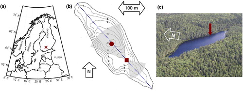
Valkea-Kotinen is a small natural lake in Southern Finland (61°14′31.02′′N, 25°3′48.83′′E) located 156 m a.s.l. with an average and maximal depth of 3 and 6 m, respectively (Futter et al., 2008, Fig. 1). The lake is very small, with an area of 4.1 ha, transversal size of about 100 m and a longitudinal size 440 m (Fig. 1b). The lake orientation is SE–NW (dashed line at Fig. 1b). The catchment of this lake is 30 ha, and it is occupied by forest surrounding the lake (Fig. 1c displays only part of the catchment, while the whole catchment can be seen in Rasilo et al., 2012, Fig. 1 therein). The presence of forest and the stretched form of the lake surface cause a wind tunnelling effect, so that prevailing wind directions fall in narrow segments around SE and NW directions (Vesala et al., 2006). The lake's bottom has significant slopes especially in the transversal direction (Fig. 1b). Lake Valkea-Kotinen is characterised by medium turbidity (Secchi disk depth is about 1 m; Arst et al., 2008) and is found to be a source of CO₂ (Huotari et al., 2011).

Fig. 1 a) Location of Lake Valkea-Kotinen (red cross) in Northern Europe. b) Bathymetry map of the lake with depth contours (m, black lines; enhanced from Kankaala et al., 2006), longitudinal size 440 m (blue dashed line), water temperature profile measurements (red circle), measurement raft (red square) and directions with acceptable flux measurements (grey transparent sectors). c) Aerial photograph of the lake also showing the raft (red arrow; Photo by Ilpo Hakala). The map of the lake catchment is given in Rasilo et al., 2012, Fig. 1 therein.

The University of Helsinki performed measurements on Lake Valkea-Kotinen in 2003–2009 (Vesala et al., 2006; Huotari et al., 2009, 2011; Nordbo et al., 2011). In this study, the year 2006 was chosen for model experiments due to the best data coverage (2 May–31 December 2006). The measurements included basic atmospheric variables (air temperature, wind speed and its direction, specific humidity, atmospheric pressure), radiation fluxes (net radiation and downward shortwave radiation) that were used to derive the forcing for lake models and detailed in Table 1; eddy covariance (EC)-based momentum, sensible and latent heat fluxes, and water temperature profiles; these were utilised for validating the models. The details on basic atmospheric variables and radiation fluxes measurements are summarised in Table 1. The gaps in forcing data series were filled using either the backup data, via a linear regression between the backup and the on-lake data, or using linear interpolation or the mean between two subsequent measurements, if the backup data were unavailable. Net radiation from mid-November until the end of the year was gap-filled by a mean diurnal course from 2007. Note, the net radiation was used only to obtain longwave radiation values (shortwave radiation sensor was functioning well). This way for gap-filling of the net radiation was chosen because (i) the nearby meteorological stations do not measure longwave radiation, and thus cannot be used, and (ii) reanalysis has typically coarse resolution in time and space (e.g. ERA-Interim has 80 km resolution in the area, 3-hour time step and the land surface scheme used in it lacks the lake tile). Regardless of the method of gap-filling, the period of concern is in the very end of the whole period of simulations and thus is unable to contribute to the model behaviour during the summer and much of the autumn. Atmospheric measurements and water thermistor string were located at the SE part and in the centre of the lake where the lake is 6 m deep, respectively (Fig. 1b). The EC system was mounted on a raft in a way to ensure that the flow from the maximal fetch directions (along the lake) would be disturbed by other devices minimally. Further details on EC data processing and fluxes calculation are reported in Nordbo et al. (2011). Due to the proximity of the lake shore (less than 50 m in NE direction), only two narrow sectors of wind directions around NW and SE were restricted by footprint considerations for EC fluxes calculation (Vesala et al., 2006). This reduced the length of EC fluxes time series by 23% and more omittance was caused by stationarity criteria (Nordbo et al., 2011), totalling in a gaps length of about 65%. The water temperature profiles were measured by thermistor chain with nominal accuracy 0.3 K and sensors located at the following depths: 0.2, 0.5, 1.0, 1.5, 1.75, 2.0, 2.25, 2.5, 2.75, 3.0, 3.25, 3.5, 4.0 m. The missing data amounted to 2.85% of the considered period.

Table 1. The meteorological forcing measured at the Lake Valkea-Kotinen

Variable	Backup data	Missing data of on-lake measurements (%)	Sensor	Nominal accuracy
Air temperature	–	0.00	Davis Vantage Pro 2	0.5°C
Wind speed	–	0.27	Metek USA1	0.05 m s^−1
Wind direction	–	0.29	Metek USA1	–
Specific humidity	Relative humidity (Iso-Evo, 5 km from the lake)	6.79	Licor LI7000	1%
Air pressure	–	6.79	Davis Vantage Pro 2	1.0 hPa
Downward shortwave radiation	–	4.73	Davis Vantage Pro 2	25 W/m^2
Downward longwave radiation	–	30.02*	Derived using net radiation (MB-1, Astrodata), shortwave radiation, surface temperature, water emissivity 0.98 and albedo 0.06	–

*Missing data is mainly from mid-November and December.

3. Lake models

The five lake models used in this study are FLake, CLM4-LISSS, LAKE, LAKEoneD and Simstrat. A short description of each model, relevant to ice-free conditions that are mostly simulated in this study, is given below, and a short summary of model features is presented in Table 2. More elaborate descriptions may be found in either original publications for each model cited below, or in Stepanenko et al. (2013).

Table 2. The summary on lake models participating in the Valkea-Kotinen experiment. See also Table A1.1 for details on parameters of k-ɛ models

Lake model, major publications	Vertical structure/number of layers in reference run (lake depth 2 m)/grid spacing (if equidistant)	Time step, s	Parameterisation of turbulent fluxes at the lake-atmosphere interface	Turbulent mixing parameterisation	Treatment of heat flux at the water-bottom sediments interface
FLake, Mironov, 2008; Mironov et al., 2010; Kirillin et al., 2011	Parameterised temperature profile/2 (top mixed layer and thermocline)	3600	Monin-Oboukhov similarity theory accounting for specific features of the surface air layer over lakes	Homogeneous temperature profile in mixed-layer and self-similarity concept in thermocline	Parameterisation of temperature profile in bottom sediments (soil) using self-similarity hypothesis
CLM4-LISSS, Hostetler and Bartlein, 1990; Subin et al., 2012; Oleson et al., 2010	Multilayer/25 layers	600	An extended scheme from CLM4 model (Oleson et al., 2010; Subin et al., 2012)	Henderson-Sellers parameterisation of eddy diffusivity, buoyant convection (Hostetler and Bartlein, 1990)	Heat conductance in bottom sediments (soil)
LAKE, Stepanenko et al., 2011	Multilayer/20	30	Monin-Oboukhov similarity theory with universal functions for stable boundary layer from (Esau and Zilitinkevich, 2006)	K-ɛ with Canuto stability functions	Heat conductance in bottom sediments (soil)
SimStrat, Goudsmit et al., 2002; Perroud et al., 2009	Multilayer/40/0.05 m	600	Empirical equations (Livingstone and Imboden, 1989; Kuhn, 1978; Dingman et al., 1968)	K-ɛ with Galperin stability functions	Zero heat flux
LAKEoneD, Jöhnk and Umlauf, 2001; Jöhnk et al., 2008	Multilayer/20/0.1 m	198	(Jöhnk, 2005)	K-ɛ with standard coefficients	Zero heat flux

FLake (Fresh-water Lake model; Mironov et al., 2010; Kirillin et al., 2011) uses a conceptual scheme of dividing the water column into two layers: the mixed layer, described by its temperature and depth, and the thermocline, in which the non-dimensional temperature profile is defined by a function of non-dimensional depth (self-similarity concept; Kitaigorodskii and Miropolsky, 1970). Substituting this profile in the heat conduction equation with radiation source yields the ordinary differential equations for mixed-layer depth, its temperature, the bottom temperature and the shape factor of thermocline. This makes the model very efficient in terms of computational time. The temperature profiles of bottom sediments, ice and snow layers are calculated using self-similarity concept as well. The radiation scheme does not treat the near infrared (NIR) and the visible parts of solar radiation separately, and after reflection according to albedo, the remaining part of solar radiation is attenuated in the water column following the Beer-Lambert law. Note that in FLake, Beer-Lambert law may be used for up to eight different wavelength bands independently, but in our simulations we set one band to make radiation treatment in FLake consistent with other models. The surface flux scheme of FLake is based on MOST theory and accounts for a number of specific lake surface features such as fetch-dependent roughness. A number of studies demonstrated that FLake captures both diurnal and seasonal cycle of surface temperature of shallow lakes satisfactorily (Mironov, 2008). Both numerical efficiency and realistic simulation of the surface temperature have brought ‘popularity’ to this model in NWP community, and it has been embedded in a number of land surface schemes (Balsamo et al., 2010; Dutra et al., 2010; Mironov et al., 2010).

The model CLM4-LISSS (Community Land Model 4–Lake, Ice, Snow, and Sediment Simulator; Subin et al., 2012) originates from the Hostetler model (Hostetler and Bartlein, 1990). It explicitly considers the heat conduction in snow, ice, water, bottom sediments and the bedrock layers. The heat conduction in water includes Henderson-Sellers formulation, wind-driven mixing, buoyant convection, the parameterised mixing by 3D circulations (Fang and Stefan, 1996) and molecular conductance. This heat conductance parameterisation does not need the explicit calculation of horizontal velocities’ profiles. The shortwave radiation is divided into NIR and visible light. The first is absorbed at the surface, and the second one except the reflected fraction, follows the Beer-Lambert law throughout the water column. The heat, moisture and momentum fluxes to the atmosphere are calculated by the surface flux scheme from CLM4 (Oleson et al., 2010).

The LAKE model (Stepanenko et al., 2011) is a k-ɛ model with shear- and stability-dependent coefficient C _t in turbulent viscosity (v _t standing for eddy viscosity, k – turbulent kinetic energy (TKE), ɛ – dissipation rate of TKE, N – Brunt-Väisälä frequency and s – shear frequency) according to Canuto et al. (2001). It solves two horizontal momentum equations, heat conductance equation, equations for turbulent kinetic energy and its dissipation rate, all including the depth dependence of horizontal cross-section area. Momentum equations account for Coriolis force and the vertical viscosity. The NIR fraction of shortwave radiation is absorbed at the surface, the rest is partially reflected and partially penetrated into the water following the Beer-Lambert law. The heat conduction and the moisture transfer including phase transitions (not relevant in this study) in the bottom sediments are implemented borrowing the formulations from the soil model of the Institute of Numerical Mathematics RAS (Volodin and Lykosov, 1998a, 1998b). The model contains the ice and snow modules, explicitly calculating the heat conductance in these layers (the liquid moisture transport in snow as well). The energy and momentum fluxes to the atmosphere are computed based on MOST theory with universal functions according to Esau and Zilitinkevich (2006).

The LAKEoneD model (Jöhnk and Umlauf, 2001; Jöhnk et al., 2008) is a k-ɛ model using standard coefficients (Rodi, 1993; Mohammadi and Pironneau, 1994). It solves five equations (two for horizontal momentum, one for heat and two equations for TKE and its dissipation rate) for horizontally averaged variables, so that area-depth dependence is taken into account explicitly. Contrary to LAKE, it does not account for Coriolis force for this study, but includes boundary friction formulated as a quadratic law with constant drag coefficient chosen according to the lake's settings (Jöhnk, 2001). The model does not include the heat transport in bottom sediments, and the bottom heat flux is set to constant (zero in this study). A simple ice model is included, in which meteorological forcing by air temperature but not lake temperature is used (Ashton, 2011). The solar radiation is treated in the same way as in LAKE and CLM4-LISSS. Sensible and latent heat fluxes to the atmosphere are calculated following Jöhnk (2005).

The Simstrat model (Goudsmit et al., 2002; Perroud et al., 2009) is a k-ɛ model with constant coefficient C _t in turbulent viscosity according to Galperin et al. (1988). As in LAKE, the Coriolis force is included in horizontal momentum equations. The equations of the model contain area-depth dependence, similar to LAKE and LAKEoneD. As in FLake, Simstrat does not distinguish between NIR and visible parts of shortwave radiation, and the shortwave radiation penetrated below the surface is attenuated exponentially with depth. The heat and momentum fluxes to the atmosphere are calculated according to empirical equations (Dingman et al., 1968; Kuhn, 1978; Livingstone and Imboden, 1989). The flux at the bottom is a prescribed constant, zero in this study. The model does not contain explicit treatment of an ice layer. To reduce heat penetration and turbulence in the water column during lake freezing periods, the model assumes that zero flux enters the lake surface when the surface water temperature drops below the freezing point and the heat flux into the lake is negative.

The parameters of the three k-ɛ models are summarised in Appendix 1. The formulation of morphometry effect is identical in all three k-ɛ models and discussed in more detail in Section 5.3.3 when interpreting the model results.

4. Experimental setup

The experimental setup in this study follows the LakeMIP protocol as described in Stepanenko et al. (2010, 2013), and hence, it will be only briefly overviewed here. Physical parameters present in all models were unified as far as possible. The extinction coefficient was estimated as 3 m⁻¹ from the mean Secchi disk depth of 1 m (Arst et al., 1999, 2008) using the Poole and Atkins formula (Poole and Atkins, 1929). The geothermal heat flux was set to 0 W/m² and applied for the lower soil boundary in FLake, CLM4-LISSS and LAKE, and to the lake bottom in LAKEoneD and Simstrat. Each model had to be run with two depths: the mean depth (3 m) and the maximal depth (6 m). Additionally, three k-ɛ models taking into account the lake morphometry were run including and excluding the lake morphometry via the hypsometric curve, as detailed in Section 5.3.3 (the bathymetry data is provided by Geological Survey of Finland). All model parameters in these experiments are listed in Table 3. All model runs were performed for the period from 00:30 (UTC+2) 2 May 2006 to 00:00 (UTC+2) 31 December 2006. No model calibration was explicitly prescribed in the setup. However, some models were calibrated, that is practically unavoidable when a lake model is being adopted for a particular lake. In the Simstrat model, the surface drag coefficient was tuned to 10⁻³ that fitted best the measured vertical temperature profiles. In LAKE, surface roughness parameter (z ₀) was found to be critical for successful reproduction of surface temperature and was set to 10⁻³ m (that falls in the typical range of open water roughness values), bringing reasonable agreement with observations for this variable, with bias of 0.08°C, and root mean square error (RMSE) approximately 1.1°C. The results of both basic and additional experiments are presented in the next section. We will also refer to the experiment with 3 m depth and neglected morphometry as a baseline (reference) one.

Table 3. The model parameters and experiments

Parameter	Value
Depth	3 m or 6 m
Extinction coefficient in water	3 m^−1
Albedo of water	0.06
Reflectivity of water for longwave radiation (‘longwave albedo’)	0
Emissivity of water	0.98
Geothermal heat flux	0 W/m^2
Lake morphometry	Basic experiment: excluded; additional experiment: included (only for k-ɛ models)

An important remark should be given in respect to surface flux schemes. It is evident that unifying the surface flux scheme among lake models would exclude the key factor of surface temperature discrepancy between models and make the surface temperature differences being caused only by the different treatment of in-lake mixing. To make such unification was initially the intention of LakeMIP project, but soon it was realised as a significant technical issue. In some models incorporating new surface flux scheme is simpler, but in others, especially those embedded in the land surface schemes of NWP or climate models, this is quite a complicated task. Therefore, all lake models so far have been allowed in previous LakeMIP studies to use native surface flux schemes. This is also the case in current intercomparisons.

5. Results and discussion

5.1. Surface temperature

The surface temperature time series for the period of model integration is shown in Fig. 2. In general, all models satisfactorily captured both diurnal and seasonal cycles of the surface temperature. The instant deviations of modelled temperature from the measured one are typically less than 2°C that may be regarded as sufficient accuracy for atmospheric applications. Indeed, this value coincides with the diurnal lake surface temperature range whereas the diurnal range of the land temperature in summer is several times larger (in 2006 diurnal air temperature range above the lake in May–July was approximately 10°C or higher for the majority of days, indicating that the diurnal course of mean surface temperature of surrounding land should be of the same magnitude). Thus, this error allows for realistic reproduction of the lake–land temperature difference during ice-free period, which is crucial for properly aggregating surface fluxes in atmospheric models.

Fig. 2 Time series of surface temperature as modelled (baseline experiment) and measured at Valkea-Kotinen Lake (2 May–31 December 2006; panel a: May–July; b: August–October; panel c: November–December). Time=0 at abscissa axis corresponds to 00:30 local time 2 May 2006. Inset at panel c presents ice thickness evolution in models for the same time period.

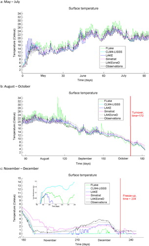
Significant outliers may be noticed only for LAKE (5–6 d in the beginning of May) and FLake (5 d in the end of August). These spikes can be caused only by the surface energy balance peculiarities. Therefore, since radiation treatment is unified between the models, only two reasons for outliers may have had place: either surface flux scheme underestimates the total heat flux to the atmosphere, or the subsurface mixing is too weak, enabling rapid radiational heating of the top model layer during daytime (for LAKE). However, when run with FLake's surface flux scheme, these spikes did not reduce substantially in LAKE, that argues for weak subsurface turbulent mixing in this model. For FLake, the most prominent spikes around 110–120 d of the model integration correspond to two times shrinking of the mixed-layer depth (not shown). This abrupt shrinking is likely to cause the positive jump of mixed-layer temperature due to mixed-layer enthalpy conservation.

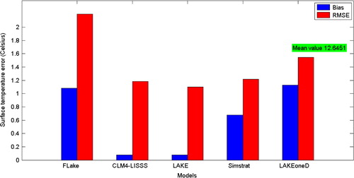
The diurnal cycle with about 2°C amplitude remains prominent until the end of September when the solar radiation drops down as well as the diurnal amplitude of surface energy fluxes (see below in this Section). Note: in November surface temperature of FLake, CLM4-LISSS and LAKE reaches zero, and ice layers form (Fig. 2c, inset). The ice also forms in LAKEoneD, but the water surface temperature remains positive, due to peculiarities of water–ice interface treatment in this model. In SimStrat, ice does not appear, as this model does not include an ice module. The biases and RMSEs for surface temperature calculated for the whole period of simulation are presented in Fig. 3. The biases of all models are positive and do not exceed 1.2°C, whereas RMSEs fall into the approximate range of 1–2°C. We do not speculate on reasons for positivity of all biases, since the two out of five are less than a nominal accuracy of water temperature sensors. It should be noted here that since radiation properties (albedo, emissivity and extinction coefficient) were unified, the difference in errors is caused by the subsurface mixing and/or the surface flux schemes implemented in the models. The importance of surface flux scheme properties can be illustrated by the fact that, if the LAKE model is run with fetch-dependent roughness parameter from FLake's scheme instead of the constant value 10⁻³ m, the surface temperature errors become close to those of FLake (the bias is 1.17°C, RMSE is 1.96°C vs. 0.08°C and 1.1°C in the baseline experiment, respectively).

Fig. 3 Surface temperature errors of lake models in a baseline experiment (blue columns – difference of means, or bias; red – RMSE). The mean temperature is indicated in a green box.

5.2. Surface heat fluxes

The mean diurnal course of modelled sensible heat flux for July and November (representative of summer and late autumn conditions) is shown in Fig. 4. Remarkably, the diurnal cycle of sensible heat flux in Fig. 4a is close to diurnal cycles for all months from May to September (not shown) as has been seen in observations as well (Nordbo et al., 2011). This flux is almost always positive indicating that the lake is warmer than the overlying air. The minimal flux is around 16:00 local time when the air–water temperature difference reduces. Nocturnal fluxes increase because the measured air temperature drops down. The latter can naturally be explained by the advection of cold air from radiatively cooled surface of the surrounding land. In October, the pattern of diurnal cycle holds but with less amplitude (not shown), and larger minimal values (ranging from 5.5 W/m² for FLake to 12.5 W/m² for LAKE) indicating the seasonal cooling of land and hence the air advected from it. Fig. 4b demonstrates reduced diurnal cycle in November and again positive values of sensible heat flux, except for LAKEoneD with almost zero values. The latter is consistent with very low values of latent heat flux in this model for the same period (Fig. 4d), both indicating for low surface heat exchange coefficients in the surface flux scheme of LAKEoneD. The only month with permanent negative sensible heat fluxes is December, for all models (ranging between models from −3.6 to −14.4 W/m²), implying this is the only month when the air was on average warmer than the lake. This leads to a gradual increase of surface temperature in the first part of December (Fig. 2c).

Fig. 4 The monthly mean diurnal cycle of sensible and latent heat flux for July and November 2006, modelled in a baseline experiment: (a) sensible heat flux, July, (b) sensible heat flux, November, (c) latent heat flux, July, and (d) latent heat flux, November.

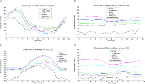
The diurnal cycle of latent heat flux is different from that of sensible heat flux (Fig. 4c). Again, as for the sensible heat flux, a similar form of this cycle with maximum around 14:00 local time is typical for the period from May to September. The maximum is evidently caused by the daily maximum of surface temperature and specific humidity close to the water surface. Starting with October the diurnal cycle of latent heat flux vanishes (Fig. 4d, November is shown).

EC fluxes are also added to Fig. 4, but we avoid discussing them thoroughly, since the EC heat fluxes time series miss about 65% of values due to stringent quality criteria. Nevertheless, one can see from Fig. 4 that the observed diurnal pattern is close to modelled and shifted towards negative values. This is consistent with systematic overestimation of observed heat fluxes by models discussed below. Notwithstanding long gaps in EC flux series, it is possible to compare EC time series with corresponding simulated series by omitting the modelled data falling in EC data gaps. The resulting biases are positive for all models and for both heat fluxes (Fig. 5a, b). Both biases and RMSEs are large compared to mean values of fluxes. This result is consistent with similar EC vs. model fluxes comparison implemented for Kossenblatter See (Stepanenko et al., 2013) and with the excess lake evaporation obtained with LAKEHTESSEL scheme for Valkea-Kotinen Lake (Manrique-Suñén et al., 2013) (LAKEHTESSEL is a FLake-based lake scheme in HTESSEL model, Dutra et al., 2010). The latter report the bias of modelled latent heat flux for summer months to be 25 W/m² similar to values in Fig. 5b. It is argued there that the systematic shift between computed fluxes and those measured by EC is likely to be caused to a large extent by the underestimation of real fluxes at the lake surface by EC technique. The main argument for that is the heat balance residual arising when the algebraic sum of measured surface energy fluxes is compared to the change of the lake heat storage (specifically, , with r – the residual, R _n – the net radiation at the lake surface, H – the sensible heat flux, LE – the latent heat flux and Q – the heat storage of the lake water column in the point of measurements). The sign of this residual is usually consistent with underestimation of heat fluxes by the EC method. A number of reasons are reported in literature for deviation of EC-fluxes from ‘real’ fluxes (i.e. derived from the lake's heat balance) at the local surface (Wilson et al., 2002; Foken et al., 2006; Foken, 2008; Nordbo et al., 2011), and given the scope of this paper they are not discussed here.

Fig. 5 Sensible heat (a) and latent heat (b) flux errors of lake models in a baseline experiment (blue columns – difference of means, or bias; red columns – RMSE; pink boxes – correlation coefficient). The mean sensible and latent heat fluxes are indicated in green boxes at (a) and (b), respectively.

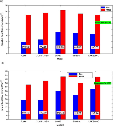
As to Lake Valkea-Kotinen, EC heat fluxes did not allow the closure of heat balance during the open-water period in 2006 with residual of 16 W/m² (Nordbo et al., 2011). Assuming that this residual is caused by errors in the EC fluxes and not in the net radiation or in change in the water heat storage, it explains 46–70% of the bias of modelled total heat flux with respect to EC data (these biases range from 23 to 35 W/m² for different models, Fig. 5a, b). The remaining part of the positive total heat flux biases may be attributed to systematic overestimation of the surface temperature by models (Fig. 3) increasing the surface fluxes, and the errors of surface flux schemes. The latter may include inter alia the violation of horizontal homogeneity of the flow for the lake bounded by forest and the surface roughness in conditions of immature wave development. We do not proceed here in the discussion of these possible contributors to fluxes’ biases since the observational data available do not form a solid basis for such an analysis. Regardless, the cause of the possible bias of EC fluxes in respect to real ones at the surface EC-fluxes obviously reflect the variability of atmospheric conditions from subdiurnal to seasonal scale and hence may be used to validate the dynamics of modelled heat fluxes. In this respect, all models showed a satisfactory skill: correlation coefficients of modelled sensible heat flux vs. EC ranged from 0.55 to 0.63, and for the latent heat flux from 0.70 to 0.74 (Fig. 5a, b).

5.3. Temperature profiles

5.3.1. General evaluation.

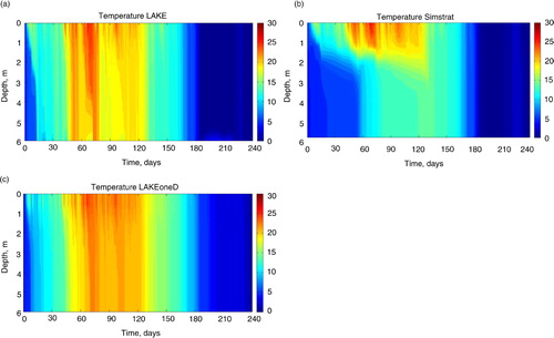
The temperature profile evolution is reproduced quite differently by lake models as seen in Fig. 6. The qualitative behaviour of stratification with top mixed heated layer in summer and intense mixing in autumn is simulated by all models. The summer stratification in CLM4-LISSS model (Fig. 6b) may be regarded as the best fitting to observations with the gradual heating of the water column until August and typical mixed-layer depth of about 1.5 m. The temperature profile in the thermocline is almost linear in this model; that is the case for measured data also (Fig. 6f). The success of this model may be attributed inter alia to specification of fetch-dependent surface parameters such as the surface roughness (Subin et al., 2012).

Fig. 6 The time evolution of temperature profiles in Valkea-Kotinen Lake according to models in a baseline experiment (a – FLake, b – CLM4-LISSS, c – LAKE, d – Simstrat, e – LAKEoneD) and observations (panel f). The temperature is given in °C, time=0 corresponds to 0:30 2 May 2006.

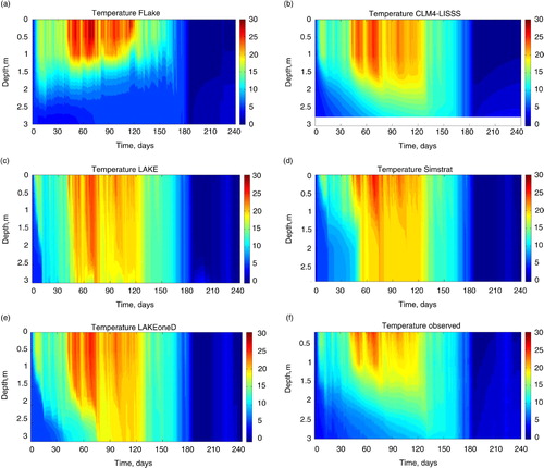
FLake model realistically reproduces the mixed-layer depth values, however, this is the only model producing mixed layer shallowing with time in July and August (Fig. 6a). This result is consistent with simulations of the Lake Valkea-Kotinen by the LAKEHTESSEL scheme (Manrique-Suñén et al., 2013) that uses FLake for vertical heat transfer in a lake. This hints to insufficient mixed-layer development in FLake under conditions of weak winds (the mean wind speed at the site was only 1.2 m/s in 2006 with speeds >5 m/s happening <5% of the open-water period time). Moreover, the thermocline in FLake is shallower than it is in observations and is bounded from beneath by hypolimnion, a cold constant-temperature layer (around 4°C) of close to 1 m thickness. This implies that the heat does not penetrate below the thermocline down to the lake bottom leaving more heat in the mixed layer and causing the positive bias of the surface temperature (Figs. 2 and 3).

All three k-ɛ models overestimated the mixing in this lake (Fig. 6c–e). The mixing in Simstrat was less intensive compared to LAKE and LAKEoneD due to reduced drag coefficient for momentum flux at the lake–atmosphere interface (see the discussion on momentum exchange with the atmosphere later in this section). In LAKE's temperature profiles, a thin stable layer is frequently present adjacent to the bottom, whereas in LAKEoneD and Simstrat there are no disturbances of temperature field near the bottom. This indicates the role of bottom sediments in LAKE that stabilise the bottom water layer by the heat loss from the water to the colder ground.

5.3.2. Drag coefficient.

Consider now the results from the experiment with 6 m depth, neglecting morphometry effects. While FLake and CLM4-LISSS produced temperature profiles very close to those from the 3 m experiment (not shown), different results were obtained for k-ɛ models (Fig. 7a–e). The LAKE model generated mixing that was too intense compared to observations (Fig. 7f), SimStrat and LAKEoneD (Fig. 7b, c). The reason for that is the high surface drag coefficient (C _d ), which is defined by the formula:1

Fig. 7 The time evolution of temperature profiles in Valkea-Kotinen Lake according to k-ɛ models in an experiment with 6 m depth neglecting morphometry (a – LAKE, b – Simstrat, c – LAKEoneD, d – LAKE with C _d =10⁻³, e – LAKE with momentum flux partitioning), and observations (panel f, the same as Fig. 8f but with different vertical scale). The temperature is given in °C, time=0 corresponds to 0:30 2 May 2006.

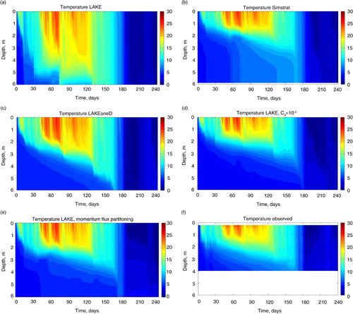
where τ is momentum flux, ρ _a is the air density and u is the wind speed. In LAKE, the drag coefficient averaged over the period of integration was 1.2·10⁻², whereas for other models its value was 1.8·10⁻³ (FLake), 4.5·10⁻³ (CLM4-LISSS), 1·10⁻³ (SimStrat) and 1.1·10⁻³ (LAKEoneD). The enhanced value of C _d in LAKE is caused by the relatively high value of surface roughness (10⁻³ m), used for best fitting the surface temperature to observations (as already mentioned above). The C _d value in CLM4-LISSS is also relatively high due to using the fetch-dependent surface roughness (Subin et al., 2012). In FLake, the fetch-dependence of surface roughness is also included, but the formulation is different (via simple empirical fetch-dependence of Charnock parameter) resulting in different values of z ₀ and, therefore, the values of C _d . The increased momentum flux from the atmosphere in LAKE leads to larger shear production of TKE in the k-ɛ scheme and thus to extra mixing. In order to verify such an hypothesis, an additional experiment was conducted with LAKE, setting a constant drag coefficient of C _d =10⁻³ and keeping the rest of the surface flux scheme unchanged. The resulting water temperature distribution (Fig. 7d) with depth is almost identical to that of SimStrat (Fig. 7b) and close to observations (Fig. 7f).

These results suggest that a 10⁻³ drag coefficient is the optimal value to reproduce the vertical mixing in water column of Valkea-Kotinen in all models, irrespective to turbulent mixing parameterisation. However, this value contradicts the mean drag coefficient derived from EC measurements at this lake that is about 7·10⁻³. Now, recall that the EC technique is likely to underestimate the real heat fluxes at the surface and, to the knowledge of authors, there is no reason to expect that momentum flux is not underestimated as well in this case (sensible heat and momentum fluxes are measured by the same device and undergo almost the same sequence of corrections, Aubinet et al., 2012). 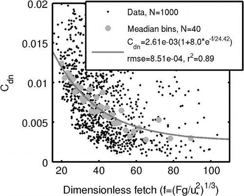Thus, since EC method provides larger values of momentum flux than that are modelled, the possibility that C _d is significantly underestimated by lake models’ surface flux schemes should be considered. The most likely reason for underestimating the drag coefficient by surface flux schemes is that they are generally unable to fully account for effects of very limited fetch complicated by the presence of forest at the lake margins. The drag coefficient for neutral stratification is known to decrease as a function of normalised fetch , where F is the fetch in meters, g gravitational acceleration and u _* friction velocity (Vickers and Mahrt, 1997 and references therein) Indeed, EC measurements demonstrate that the drag coefficient for neutral stratification C _dn approaches the value of 2.6·10⁻³ predicted by surface flux schemes at larger f (Fig. 8). Thus, the question is what might be the process consuming a significant part of momentum flux from the atmosphere, so that the remaining part of this flux does not cause overmixing of the water column.

Fig. 8 The surface drag coefficient for neutral stratification (C _dn ) as a function of dimensionless wind fetch, according to EC measurements at the Lake Valkea-Kotinen. Number of data points (N) and a fit to median values are given in the legend. The 90% confidence limits of the fitting coefficients are 0.0013–0.0040, 4.8–11.3 and 16.2–32.6.

It is known that for small water bodies (Wüest and Lorke, 2003), the surface wave field does not reach equilibrium with air flow, so that the momentum flux from the atmosphere is partitioned between wave development and acceleration of the lake's currents. This is certainly the case for Lake Valkea-Kotinen due to its small size. In order to test the hypothesis that this physical effect plays a significant role, a momentum flux partitioning parameterisation (Appendix 2) was introduced in LAKE model following parameterisations suggested in Lin et al. (2002) and Kitaigorodskii and Volkov (1965). This parameterisation includes wind fetch that is set to a constant value of 100 m. The resulting temperature profiles may be seen in Fig. 7e, where the effect of momentum flux partitioning appears to be almost the same as reducing the drag coefficient (Fig. 7d). This supports the momentum flux partitioning to be an important mechanism and suggests that the errors of underestimating the surface drag coefficient by surface flux schemes and of omitting flux partitioning in other lake models largely compensate each other. However, further research is needed to check this proposition, for example, running the model with fetch dependent on wind direction.

5.3.3. Morphometry effect.

Further, an additional experiment was done with k-ɛ models, in which the lake morphometry was taken into account. Lake Valkea-Kotinen is characterised by significant bottom slopes throughout its area (Fig. 1b), so that the effects of morphometry are anticipated to be significant. Temperature profiles shown in Fig. 9 demonstrate much more intense heating in k-ɛ models below the thermocline compared to experiments with constant lake area (independent on depth). In order to explain this result, let us consider the balance equation for horizontally averaged lake temperature:2

Fig. 9 The time evolution of temperature profiles in Valkea-Kotinen Lake according to k-ɛ models in an experiment with 6 m depth including morphometry (a – LAKE, b – Simstrat, c – LAKEoneD). The temperature is given in °C, time=0 corresponds to 0:30 2 May 2006.

where T – water temperature, averaged over the horizontal cross-section of area A, S – shortwave radiation penetrated into the water column (assumed to be constant in the cross-section), k _T – temperature conductance, – the heat flux into the bottom at the lake margins at depth z, ρ ₀ – reference water density, c _p – specific heat of water at constant pressure and the vertical coordinate z points downwards. The second term on the r.h.s. of eq. (2) is neglected in LAKE, SimStrat and LAKEoneD. Then, expanding the first term yields:3

The last term on the r.h.s. of eq. (3), which is responsible for morphometry effects, is always positive below the well-mixed layer of a lake in summertime because 0 and  0. Thus, including morphometry adds extra heating that is seen in Fig. 9. The physical cause of this effect is that when accounting for bathymetry data, the given heat flux from above at every depth z heats up the lesser water volume than in the case of constant lake cross-section when the effect of bottom sediments is neglected [2-d term in the r.h.s. of eq. (2)]. Therefore, for this particular lake the heat flux at the lake margins in eq. (2) cannot be omitted in order to represent vertical temperature profiles realistically.

6. Conclusions

Five 1D lake models with different turbulence closures, surface flux parameterisations and bottom sediment treatments were run for the open water season in 2006 for Lake Valkea-Kotinen (Finland) using on-lake measured meteorological forcing. The model results were validated using water temperature measurements and EC fluxes.

The surface temperature is satisfactorily simulated by all models, however, showing occasional spikes and consistent but small (by 0.1°C–1.1°C) overestimation. Both of the averaged sensible and latent heat fluxes are overestimated by all models respective to EC data. This is consistent with a similar model study for Kossenblatter Lake (Stepanenko et al., 2013). Between 46 and 70% (for different models) of this systematic bias may be explained by the bias of EC measurements itself in respect to the total heat flux derived from the lake's heat balance. On the other hand, correlation coefficients between EC-fluxes and those simulated are relatively high ranging from 0.55 to 0.63 for sensible heat, and for the latent heat from 0.70 to 0.74. As to lake stratification, the results from CLM4-LISSS model correspond reasonably well to observations. FLake model simulates realistic values of mixed-layer depth but this depth shallows with time in July and August contrary to other models and observations. This is likely due to insufficient vertical mixing in this model in weak wind conditions, characterising the Lake Valkea-Kotinen. The models including k-ɛ turbulence closure (LAKE, SimStrat, and LAKEoneD) produced similar depth-time temperature pattern that is, however, sensitive to the choice of the surface drag coefficient. By tuning this coefficient to 10⁻³ in LAKE and SimStrat, realistic temperature profiles were obtained. However, this drag coefficient is several times less than that measured by EC system (C _d =7·10⁻³).

It is proposed that the surface flux schemes of lake models underestimate the drag coefficient in conditions of limited fetch and the presence of forest around the lake, but a part of momentum flux is consumed by wave development (Wüest and Lorke, 2003). Adopting the simple parameterisation for momentum flux partitioning in LAKE model, indeed, significantly reduced the vertical mixing, suggesting that misrepresenting both enhanced drag over the small forest-bounded lake and momentum flux partitioning compensate each other in lake models to simulate realistic temperature distribution with depth.

Finally, the effect of including the lake bathymetry data in k-ɛ models was studied. Including morphometry enhanced the water heating below the thermocline dramatically. This is caused by omitting the heat flux in all models at the lake margins that appears in the horizontally averaged temperature equation. Thus, the parameterisation of heat flux at the lake's margins should be included in the models, otherwise it is recommended to neglect bathymetry effects.

Acknowledgements

We acknowledge Dr. Jussi Huotari and Dr. Anne Ojala for conducting the measurements. Lake morphometric data were provided by Geological Survey of Finland. V. Stepanenko was supported by grants from the Russian Foundation for Basic Research (RFBR 12-05-01068, 11-05-01190), Council of President of Russian Federation for support of young Russian scientists and leading research schools MK-6767.2012.5, and the Russian Ministry for Education and Science, agreement No.8336. A. Nordbo and I. Mammarella acknowledge funding from the Academy of Finland Centre of Excellence program (project No. 1118615), the Academy of Finland ICOS project (263149), the EU ICOS project (211574), EU GHG-Europe project (244122) and the Nordic Centre of Excellence project DEFROST.

8. Appendices

Appendix 1. The parameters of k-ɛ models

The equations of k-ɛ turbulence closure used in LAKE, SimStrat and LAKEoneD are:A1.1

Here, z axis points downwards, k – turbulent kinetic energy (TKE), ɛ – dissipation of TKE, P – shear production of TKE, B – buoyancy production of TKE, u and v are the horizontal components of speed, v – molecular viscosity, v _t – eddy viscosity, v _t,ρ – eddy diffusivity for temperature and other scalars, ρ – water density, ρ ₀ – reference water density, g – acceleration due to gravity. Table A1.1 presents the parameters used in eq. (A1.1) in all three models.

Table A1.1. The parameters of k-ɛ models

Parameter	LAKE	LAKEoneD	Simstrat
σ k	1	1	1
σ ɛ	1.111 (fulfilling the law of the wall, Burchard, 2002)	1.3	1.3
σ 1ɛ	1.44	1.44	1.44
σ 2ɛ	1.92	1.92	1.92
σ 3ɛ	1.14 if B>0 −0.4 if B<0	0.8	1 if B>0 −0.4 if B<0
C t	Stability function for momentum (Canuto et al., 2001)	0.09	0.09 (C constant, Galperin et al. (1988))
C t,ρ	Stability function for scalars (Canuto et al., 2001)	0.09	0.11 (C constant, Galperin et al. (1988))
Boundary conditions at the water–air interface	For TKE, the no-flux condition (Burchard et al., 1998), for dissipation the flux boundary condition of Burchard and Petersen (1999)	Dirichlet boundary conditions assuming local equilibrium (Svensson, 1978; Rodi, 1993)	For TKE, the no-flux condition (Burchard et al., 1998), for dissipation the flux boundary condition of Burchard and Petersen (1999)
Boundary conditions at the lake bottom	As above	As above	As above

Appendix 2. Momentum flux partitioning

The total momentum flux from the atmosphere, τ, is partitioned into the flux feeding the wave development, τ _wave, and the flux accelerating the currents in the surface boundary layer (SBL), τ _SBL (Wüest and Lorke, 2003):A2.1

Here τ is calculated from the surface flux scheme of a lake model. Thus, τ _SBL can be found from (A2.1), and is used in boundary conditions for momentum equations. However, we now need a parameterisation for τ _wave. Following (Kitaigorodskii and Volkov, 1965; Lin et al., 2002), one can write:A2.2

where ρ _a – the air density, C – the mean wave phase speed, C _wave,10 – the surface drag coefficient for 10 m height, u ₁₀ – the wind speed at 10 m over the lake. The difference of formulation used here from that by (Lin et al., 2002) is that C _wave,10 is calculated by surface flux scheme of LAKE model, i.e. including effects of stratification, whereas in (Lin et al., 2002) it is given by a logarithmic law. For the mean wave speed we use the relation with dominant wave speed (C _p ), C=0.83C _p (e.g. Wüest and Lorke, 2003). To estimate the dominant wave speed, we adopt the equations for significant wave height by Hasselmann (Hasselmann et al., 1973; Wüest and Lorke, 2003):A2.3

that can be combined inA2.4

with u _*a – the friction velocity in air, g – the acceleration due to gravity, F – the wind fetch, and c ₁ =0.051, c ₂ =0.96, being empirical constants.

References

- Arst H , Erm A , Herlevi A , Kutser T , Leppäranta M. A , co-authors . Optical properties of boreal lake waters in Finland and Estonia. Boreal Environ. Res. 2008; 13: 133–158.
- Arst H , Erm A , Kallaste K , Mäekivi S , Reinart A , co-authors . Investigation of Estonian and Finnish lakes by optical measurements in 1992–9. Proc. Estonian Acad. Sci. Biol. Ecol. 1999; 48: 5–24.
- Ashton G. D . River and lake ice thickening, thinning and snow ice formation. Cold Regions Sci. Techn. 2011; 68: 3–19.
- Aubinet M , Feigenwinter C , Heinesch B , Laffineur Q , Papale D , co-authors . Aubinet M , Vesala T , Papale D . Nighttime flux correction. Eddy Covariance: A Practical Guide to Measurement and Data Analysis Series: Springer Atmospheric Sciences. 2012; Dordrecht, Heidelberg, London, New York: Springer. XXII, 438p. 90 illus., 38 illus. in color.
- Balsamo G , Dutra E , Stepanenko V. M , Viterbo P , Miranda P. M. A , Mironov D . Deriving an effective lake depth from satellite lake surface temperature data: a feasibility study with MODIS data. Boreal Environ. Res. 2010; 15: 178–190.
- Balsamo G , Salgado R , Dutra E , Boussetta S , Stockdale T , co-authors . On the contribution of lakes in predicting near-surface temperature in a global weather forecasting model. Tellus. Dyn. Meteorol. Oceanogr. 2012; 64: 15829.
- Burchard H . Applied Turbulence Modeling in Marine Waters. 2002; Berlin: Springer-Verlag. 215.
- Burchard H , Petersen O . Models of turbulence in the marine environment—a comparative study of two-equation turbulence models. Mar. Syst. 1999; 21: 29–53.
- Burchard H , Petersen O , Rippeth T . Comparing the performance of the Mellor-Yamada and the k-ɛ two-equation turbulence models. J. Geophys. Res. 1998; 103: 10,543–10,554.
- Canuto V. M , Howard A , Cheng Y , Dubovikov M. S . Ocean turbulence. Part I: one-point closure model. Momentum and heat vertical diffusivities. J. Phys. Oceanorgr. 2001; 31: 1413–1426.
- Dingman S. L , Weeks W. F , Yen Y. C . The effects of thermal pollution on river ice conditions. Water Resour. Res. 1968; 4: 349–362.
- Dutra E , Stepanenko V. M , Balsamo G , Viterbo P , Miranda P. M. A , co-authors . An offline study of the impact of lakes on the performance of the ECMWF surface scheme. Boreal Environ. Res. 2010; 15: 100–112.
- Esau I , Zilitinkevich S . Universal dependences between turbulent and mean flow parameters in stably and neutrally stratified planetary boundary layers. European Geophysical Society. Nonlinear Processes Geophys. 2006; 13: 135–144.
- Fang X , Stefan H. G . Long-term lake water temperature and ice cover simulations/measurements. Cold Reg. Sci. Techn. 1996; 24: 289–304.
- Foken T . The energy balance closure problem: an overview. Ecol. Appl. 2008; 18(6): 1351–1367.
- Foken T , Wimmer F , Mauder M , Thomas C , Liebethal C . Some aspects of the energy balance closure problem. Atmos. Chem. Phys. 2006; 6: 4395–4402.
- Futter M. N , Starr M , Forsius M , Holmberg M . Modelling effects of climate on long-term patterns of dissolved organic carbon concentrations in the surface waters of a boreal catchment. Hydrol. Earth Syst. Sci. 2008; 12: 437–447.
- Galperin B , Kantha L , Hassid S , Rosati A . A quasi-equilibrium turbulent energy model for geophysical flows. J. Atmos. Sci. 1988; 45: 55–62.
- Goudsmit G.-H , Burchard H , Peeters F , Wüest A . Application of k-ɛ model to enclosed basins: the role of internal seiches. J. Geophys. Res. 2002; 107(C12): 3230.
- Hasselmann K , Barnett T. P , Bouws E , Carlson H , Cartwright D. E , co-authors . Measurements of wind-wave growth and swell decay during the Joint North Sea Wave Project (JONSWAP). Dtsch. Hydrog. Z. Suppl. A. 1973; 8: 95.
- Hostetler S , Bartlein P . Simulation of lake evaporation with application to modeling lake level variations of Harney-Malheur Lake, Oregon. Water Resour. Res. 1990; 26: 2603–2612.
- Huotari J , Ojala A , Peltomaa E , Nordbo A , Launiainen S , co-authors . Long-term direct CO(2) flux measurements over a boreal lake: five years of eddy covariance data. Geophys. Res. Lett. 2011; 38: L18401.
- Huotari J , Ojala A , Peltomaa E , Pumpanen J , Hari P , co-authors . Temporal variations in surface water CO2 concentration in a boreal humic lake based on high-frequency measurements. Boreal Environ. Res. 2009; 14: 48–60.
- Jöhnk K. D . 1D hydrodynamic models in limnophysics (Turbulence - Meromixis - Oxygen). Habilitationschrift. Limnophysics Rep. 2001; 1(1): 1–235.
- Jöhnk K. D , Lehr J. H , Keeley J . Heat balance of open water bodies. Water Encyclopedia, Vol. 3: Surface and Agricultural Water. 2005; Hoboken, New Jersey: John Wiley & Sons. 190–193.
- Jöhnk K. D , Huisman J , Sommeijer B , Sharples J , Visser P. M , Stroom J . Summer heatwaves promote blooms of harmful cyanobacteria. Glob. Change Biol. 2008; 14: 495–512.
- Jöhnk K. D , Umlauf L . Modelling the metalimnetic oxygen minimum in a medium sized alpine lake. Ecol. Model. 2001; 136: 67–80.
- Kankaala P , Huotari J , Peltomaa E , Saloranta T , Ojala A . Methanotrophic activity in relation to methane efflux and total heterotrophic bacterial production in a stratified, humic, boreal lake. Limnol. Oceanogr. 2006; 51: 1195–1204.
- Kitaigorodskii S. A , Miropolsky Y. Z . On the theory of the open ocean active layer. Izv. Akad. Nauk SSSR. Fizika Atmosfery i Okeana. 1970; 6: 178–188.
- Kitaigorodskii S. A , Volkov Y. A . On the roughness parameter of the sea surface and the calculation of momentum flux in the nearwater layer of the atmosphere. Izv. Atmos. Oceanic Phys. 1965; 1: 973–988.
- Kirillin G , Hochschild J , Mironov D , Terzhevik A , Golosov S , Nützmann G . FLake-global: online lake model with worldwide coverage. Environ. Model. Software. 2011; 26: 683–684.
- Kuhn W . Evaporation from Lake Zuerich calculated from climate data and the heat budget. Vierteljahrschrift der naturforschenden Gesellschaft in Zürich. 1978; 123: 261–283.
- Lin W , Sanford L. P , Suttles S. E , Valigura R . Drag coefficients with fetch-limited wind waves. J. Phys. Oceanogr. 2002; 32: 3058–3074.
- Livingstone D. M , Imboden D. M . Annual heat balance and equilibrium temperature of Lake Aegeri, Switzerland. Aquat. Sci. 1989; 51: 351–369.
- Long Z , Perrie W , Gyakum J , Caya D , Laprise R . Northern lake impacts on local seasonal climate. J. Hydrometeorol. 2007; 8: 881–896.
- MacKay M . A process-oriented small lake scheme for coupled climate modeling applications. J. Hydrometeor. 2012; 13: 1911–1924.
- Manrique-Suñén A , Nordbo A , Balsamo G , Beljaars A , Mammarella I . Representing land surface heterogeneity: offline analysis of the tiling method. J. Hydrol. 2013; 14(3): 850–867.
- Mironov D , Heise E , Kourzeneva E , Ritter B , Schneider N , Terzhevik A . Implementation of the lake parameterization scheme FLake into the numerical weather prediction model COSMO. Boreal Environ. Res. 2010; 15: 218–230.
- Mironov D. V . Parameterization of Lakes in Numerical Weather Prediction. Description of a Lake Model. 2008; Germany: Offenbach am Main. 41. COSMO Technical Report, No. 11, Deutscher Wetterdienst.
- Mohammadi B , Pironneau O . Analysis of the K-Epsilon Turbulence Model. 1994; Chichester, UK: Wiley & Sons.
- Nordbo A , Launiainen S , Mammarella I , Leppäranta M , Huotari J , co-authors . Long-term energy flux measurements and energy balance over a small boreal lake using eddy covariance technique. J. Geophys. Res. 2011; 116: D02119.
- Oleson K. W , Lawrence D. M , Bonan G. B , Flanner M. G , Kluzek E , co-authors . Technical Description of Version 4.0 of the Community Land Model (CLM). 2010; Boulder, CO: National Center for Atmospheric Research. 257. NCAR/TN-478+STR.
- Perroud M , Goyette S , Martynov A , Beniston M , Anneville O . Simulation of multiannual thermal profiles in deep Lake Geneva: a comparison of one-dimensional lake models. Limnol. Oceanogr. 2009; 54: 1574–1594.
- Poole H. H , Atkins W. R. G . Photo-electric measurements of submarine illumination throughout the year. J. Mar. Biol. Assoc. 1929; 16: 297–324.
- Rasilo T , Ojala A , Huotari J , Pumpanen J . Rain induced changes in carbon dioxide concentrations in the soil–lake–brook continuum of a boreal forested catchment. Vadose Zone J. 2012; 11(2): Online at: https://www.soils.org/publications/vzj/abstracts/11/2/vzj2011.0039 .
- Rodi W . Turbulence Models and their Application in Hydraulics – A State of The Art Review. 1993; Rotterdam: A. A. Baalkema. 104. 3rd ed.
- Samuelsson P , Kourzeneva E , Mironov D . The impact of lakes on the European climate as simulated by a regional climate model. Boreal Environ. Res. 2010; 15: 113–129.
- Stepanenko V. M , Goyette S , Martynov A , Perroud M , Fang X , co-authors . First steps of a Lake Model Intercomparison Project: LakeMIP. Boreal Environ. Res. 2010; 15: 191–202.
- Stepanenko V. M , Machul'skaya E. E , Glagolev M. V , Lykosov V. N . Numerical modeling of methane emissions from lakes in the permafrost zone. Izv. AN. Fiz. Atmos. Ok+. 2011; 47: 275–288.
- Stepanenko V. M , Martynov A , Jöhnk K. D , Subin Z. M , Perroud M , co-authors . A one-dimensional model intercomparison study of thermal regime of a shallow turbid midlatitude lake. Geosci. Model Dev. 2013; 6: 1337–1352.
- Subin Z. M , Riley W. J , Mironov D . An improved lake model for climate simulations: model structure, evaluation, and sensitivity analyses in CESM1. J Adv Model Earth Syst. 2012; 4(1): Quarter 1.
- Svensson U . A Mathematical Model of the Seasonal Thermocline. 1978; Imperial college, London. PhD thesis.
- Thiery W , Stepanenko V. M , Fang X , Jöhnk K. D , Li Z , co-authors . LakeMIP Kivu: evaluating the representation of a large, deep tropical lake by a set of one-dimensional lake models. Tellus A. 2013. in review.
- Vesala T , Huotari J , Rannik Ü , Suni T , Smolander S , co-authors . Eddy covariance measurements of carbon exchange and latent and sensible heat fluxes over a boreal lake for a full open-water period. J. Geophys. Res. 2006; 111: D11101.
- Vickers D , Mahrt L . Fetch limited drag coefficients. Bound. Layer Meteorol. 1997; 85: 53–79.
- Volodin E. M , Lykosov V. N . Parametrization of heat and moisture transfer in the soil–vegetation system for use in atmospheric general circulation models: 1. Formulation and simulations based on local observational data. – Izvestiya. Atmos. Ocean. Phys. 1998a; 34(4): 405–416.
- Volodin E. M , Lykosov V. N . Parametrization of heat and moisture transfer in the soil–vegetation system for use in atmospheric general circulation models: 2. Numerical experiments in climate modeling. – Izvestiya. Atmos. Ocean. Phys. 1998b; 34(5): 559–569.
- Wilson K , Goldstein A , Falge A , Aubinet M , Baldocchi D , co-authors . Energy balance closure at FLUXNET sites. Agric. For. Meteorol. 2002; 113: 223–243.
- Wüest A , Lorke A . Small-scale hydrodynamics in lakes. Annu. Rev. Fluid Mech. 2003; 35(1): 373–412.