LakeMIP Kivu: evaluating the representation of a large, deep tropical lake by a set of one-dimensional lake models

Abstract

The African great lakes are of utmost importance for the local economy (fishing), as well as being essential to the survival of the local people. During the past decades, these lakes experienced fast changes in ecosystem structure and functioning, and their future evolution is a major concern. In this study, for the first time a set of one-dimensional lake models are evaluated for Lake Kivu (2.28°S; 28.98°E), East Africa. The unique limnology of this meromictic lake, with the importance of salinity and subsurface springs in a tropical high-altitude climate, presents a worthy challenge to the seven models involved in the Lake Model Intercomparison Project (LakeMIP). Meteorological observations from two automatic weather stations are used to drive the models, whereas a unique dataset, containing over 150 temperature profiles recorded since 2002, is used to assess the model's performance. Simulations are performed over the freshwater layer only (60 m) and over the average lake depth (240 m), since salinity increases with depth below 60 m in Lake Kivu and some lake models do not account for the influence of salinity upon lake stratification. All models are able to reproduce the mixing seasonality in Lake Kivu, as well as the magnitude and seasonal cycle of the lake enthalpy change. Differences between the models can be ascribed to variations in the treatment of the radiative forcing and the computation of the turbulent heat fluxes. Fluctuations in wind velocity and solar radiation explain inter-annual variability of observed water column temperatures. The good agreement between the deep simulations and the observed meromictic stratification also shows that a subset of models is able to account for the salinity- and geothermal-induced effects upon deep-water stratification. Finally, based on the strengths and weaknesses discerned in this study, an informed choice of a one-dimensional lake model for a given research purpose becomes possible.

• lake modelling
• model intercomparison
• surface–atmosphere interactions
• tropical lakes
• Lake Kivu

1. Introduction

In regions where lakes compose a large fraction of the earth surface, they form an important component of the climate system. The strong contrasts in albedo, surface roughness and heat capacity between land and water modify the surface–atmosphere exchanges of moisture, heat and momentum over lakes compared to adjacent land (Bonan, 1995). Some reported effects of this modified exchange are the dampened diurnal temperature range over lakes (Subin et al., 2012a), the enhanced evaporation or even a persistent unstable atmospheric boundary layer (Verburg and Antenucci, 2010), the resulting increased precipitation downwind of the lake (Lauwaet et al., 2011), the stronger winds due to higher wind fetch (Subin et al., 2012a), and the formation of local diurnal winds (Savijärvi, 1997; Verburg and Hecky, 2003).

Given the significant impact of lakes on surface–atmosphere interactions, the need for an accurate representation of lake surface temperatures in Numerical Weather Prediction systems (NWP), Regional Climate Models (RCM) and General Circulation Models (GCM) arises. Although a multitude of one-dimensional lake models developed in the past may be a candidate to represent lake–atmosphere exchanges, only a subset of these models has been interactively coupled to atmospheric prediction models so far (Hostetler et al., 1994; Bonan, 1995; Song et al., 2004; Kourzeneva et al., 2008; Mironov et al., 2010; Davin et al., 2011; Balsamo et al., 2012; Goyette and Perroud, 2012; Martynov et al., 2012; Akkermans et al., 2014). Computational efficiency of the lake parameterisation scheme is often decisive for the choice of the scheme. A comparative assessment of different one-dimensional lake models, with emphasis on the strengths and weaknesses with respect to specific research goals, could however favour an informed choice.

From this need, in 2008 the Lake Model Intercomparison Project (LakeMIP) emerged. In a first stage, this project aims at a comparison of the thermodynamic regime of a wide range of climatic conditions and mixing regimes by a number of one-dimensional lake models (Stepanenko et al., 2010). Inspired by a model intercomparison study for the deep lake Geneva (Perroud et al., 2009), LakeMIP focused on a number of test cases such as, for mid-latitudes, the small Lake Sparkling (Stepanenko et al., 2010) and the shallow turbid Lake Kossenblatter (Stepanenko et al., 2012), whereas for a boreal climate, the small Lake Valkea-Kotinen was investigated (Stepanenko et al., 2013).

However, despite the abundance of lakes in tropical regions such as East Africa and Indonesia, up to now a lake model intercomparison study has never been conducted for an equatorial lake. In tropical climates, the limited seasonal cycle of both air temperature and incoming shortwave radiation makes way for other factors to control the mixing regime. With the meteorological controls on a lake's mixing regime and its water temperatures varying between climate zones, the need arose to conduct a model intercomparison experiment for a tropical lake.

Consequently, in this study, for the first time a set of one-dimensional lake models is evaluated over an East African lake: Lake Kivu (2.28°S; 28.98°E). Lake Kivu's meromictic mixing regime clearly differs from lakes previously studied within the project, that is, monomictic, dimictic or polymictic lakes with seasonal complete or partial ice cover. Furthermore, given the influence of salinity, dissolved gasses and geothermal springs on the characteristics of the hypolimnion, the modelling of Lake Kivu presents a worthy challenge to the one-dimensional lake models currently involved in LakeMIP. Finally, as a consequence of its distinct characteristics, Lake Kivu is among the best-studied lakes in the African Great Lakes region. Anthropogenic influences and recurrent natural hazards call for a close monitoring of the lake's physical and biological characteristics. For instance, when lava flowed into the lake after a major eruption of the near-shore Nyiragongo volcano, no significant impact on the water column stability was recorded (Lorke et al., 2004). In contrast, effects on density stratification of the emerging industrial methane extraction from lake Kivu are expected and will critically depend on the reinjection depth of the deep waters after the methane harvest (Descy et al., 2012; Wüest et al., 2012). To meet these and other challenges, a comprehensive dataset containing observed lake temperatures, Secchi depths and many other variables has been compiled over the last decade.

The two main goals of this study are: (i) the evaluation of the seasonal and inter-annual variability of Lake Kivu's thermal structure as represented by a set of one-dimensional lake models, and (ii) the assessment of the ability of the different models to simulate the effects of salinity, chemical composition and geothermal energy sources upon deep water stratification. This was done by performing two sets of simulations, one including only the freshwater mixed layer and another one for the whole lake including salinity, chemical and geothermal effects in the equation of state.

In the next section, an overview of the participating one-dimensional lake models is provided, together with a description of the observational dataset and the experimental setup. Section 3 describes the results of the intercomparison, with emphasis on the ability of the different models to reproduce Lake Kivu's mixing cycle, the surface energy exchange and the deep-water stratification. Finally, in Section 4, different options to improve individual model performance are discussed, and the validity of the horizontal homogeneity assumption is investigated.

2. Data and methods

2.1. Lake models

Seven one-dimensional lake models participate in the LakeMIP-Kivu experiment (Table 1). Time step, number of horizontal layers and their interspacing used by the different models are listed in Table 1, including the Central Processing Unit (CPU) time needed to conduct a single simulation. All models compute lake water temperatures and heat, water and momentum exchange between the lake surface and the overlying atmosphere from basic meteorological quantities. A short description of the different models is given below; for more extensive overviews, one is referred to Perroud et al. (2009), Stepanenko et al. (2012) and references herein.

Table 1. Participating one-dimensional lake models and numerical model settings used in this study for Kamembe meteorology runs on a 60 and 240 m depth grid

Lake model	No. of layers	Layer thickness (m)	Time step (min)	CPU time (Kamembe 60 m; 2557 d)*
Hostetler	60	1	60	6.1 s
SimStrat	60/240	1	10	20.5 s
LAKEoneD	60/240	1	5	52.5 s
LAKE	40/40	1.5/6	20	226.0 s
FLake	2	/	60	1.7 s
MINLAKE2012	65/80	1/5	60	8.3 s
CLM4-LISSS	25	Irregular	30	150.0 s

Note that MINLAKE2012 includes fine layer spacing in the first 1 m to facilitate the ice formation prediction. *All CPU times were measured on an Intel Core i5 processor (2.27 GHz), except for CLM4-LISSS (2.1 GHz AMD Magny-Cours processor), a model tailored for a supercomputing environment and therefore not easily portable to a single-processor machine.

The Hostetler model (Hostetler et al., 1993) includes semi-empirical formulations for the buoyant convection and wind-driven eddy turbulence mixing, adding to the thermal conductivity and molecular diffusion in a multi-layered water column. A second model, the Lake, Ice, Snow and Sediment Simulator within the Community Land Model 4 (CLM4-LISSS; Subin et al., 2012b) is originally based on the Hostetler model, but has undergone major improvements since its first inclusion in CLM2 (Bonan et al., 2002). The now comprehensive treatment of lake snow and ice, bottom sediments, lake depth and surface–atmosphere exchange significantly improved the model's performance, for shallow to medium-depth small lakes as well as for large, deep lakes (Subin et al., 2012b).

Three models belong to the class of k-ɛ turbulence closure models: LAKEoneD (Jöhnk and Umlauf, 2001; Jöhnk, 2013), SimStrat (Goudsmit et al., 2002) and LAKE (Stepanenko and Lykosov, 2005). They encompass a more sophisticated representation of the turbulent diffusivity (D _turb ) at a certain depth and time through the relation D _{turb ⁼} ck ²/ɛ, where k is the turbulent kinetic energy, ɛ the turbulent dissipation rate and c either a constant or a stability function, depending on the models (Stepanenko et al., 2012). Although k-ɛ models formally employ identical model equations, some differences in water temperature distribution are expected, given the variations in the coefficients used in the k-ɛ equations, and given the model-dependent treatment of the heat exchange with the overlying atmosphere and underlying bottom sediments.

In contrast to other participating models, that are multi-layered finite difference models, FLake (Mironov, 2008) is a two-layer bulk model, employing the concept of self-similarity to parameterise the temperature-depth curve. FLake consists of a mixed layer of constant temperature and an underlying thermocline down to the lake bottom, the latter parameterised through a fourth-order polynomial depending on a shape coefficient. The mixed layer depth is computed depending on convective entrainment and wind-driven mixing.

Next, MINLAKE2012 presents an update of MINLAKE96 (Fang and Stefan, 1996), used in previous intercomparison experiments. The model solves the one-dimensional, unsteady heat transfer equation using empirical formulations for the variable vertical diffusion coefficient and the heat exchange between water and bottom sediments (Fang and Stefan, 1996). The most important upgrades compared to MINLAKE96 are the conversion to a user-friendly spreadsheet environment and the introduction of variable temporal resolution, allowing to run the model at an hourly time step in contrast to the daily time step previously applicable.

2.2. Observations

2.2.1. Study area

Lake Kivu (01°35′S–02°30′S 028°50′E–029°23′E; 2370 km² surface area; 485 m maximum depth; 1463 m a.s.l.) is located on the border between Rwanda and the Democratic Republic of Congo, and is one of the seven African Great Lakes (Fig. 1). It drains into the Ruzizi, which flows south towards Lake Tanganyika. Below an oxic mixolimnion, which deepens to 60–70 m during the dry season, the monimolimnion is found rich in nutrients and dissolved gases, in particular carbon dioxide and methane (Fig. 2; Degens et al., 1973; Borgès et al., 2011; Descy et al., 2012). Due to the input of heat and salts from deep geothermal springs, temperature and salinity in the monimolimnion increase with depth (Degens et al., 1973; Spigel and Coulter, 1996; Schmid et al., 2005). Lake Kivu's surface water temperatures vary less compared to African Great Lakes located further away from the equator.

Fig. 1 Lake Kivu with situation of the Ishungu evaluation site and the Kamembe Weather Station (WS Kamembe) and Automatic Weather Station Bukavu (WS Bukavu).

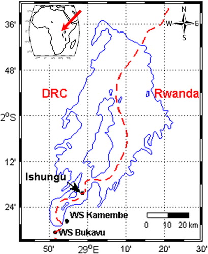
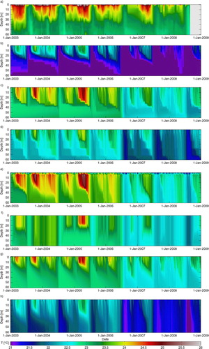
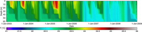
Fig. 2 Lake water temperatures (°C) at Ishungu (Lake Kivu), 2003–2008: (a) from observations, and as predicted by the models: (b) Hostetler, (c) LAKEoneD, (d) SimStrat, (e), LAKE, (f) FLake, (g) MINLAKE2012, (h) CLM4-LISSS.

2.2.2. Model forcing data

The Kamembe airport Weather Station (WS Kamembe; 02°27′31′′S–028°54′30′′E, 1591 m a.s.l.) is used to force the participating lake models. It is situated approximately 1.5 km from the lakeshore and 15 km southwest of the lake monitoring site Ishungu, but is assumed representative for meteorological conditions over this sub-basin. The station records air temperature, T (K); relative humidity, RH (%); air pressure, P (Pa), at three-hourly resolution throughout the whole day; wind velocity, u (m s⁻¹), and direction, WD (°), at hourly resolution from 6 to 18 UTC (assumed at 4 m height); and precipitation P (mm d⁻¹) at daily resolution. Although it contains only small data gaps during the integration period (January 2002–December 2008), it does not record incoming shortwave radiation SW _in (W m⁻²) and incoming longwave radiation LW _in (W m⁻²), input variables necessary to run the lake models. Hence, both SW _in and LW _in data were obtained from the ERA-Interim (Dee et al., 2011) grid point closest to the Ishungu evaluation site and converted from six-hourly accumulated values to hourly instantaneous values. After linearly interpolating T, RH and p from three-hourly to hourly resolutions, and assuming that the different meteorological variables show only little spatial variability over short distances, data gaps at WS Kamembe were filled with corresponding recordings from an Automatic Weather Station in Bukavu (WS Bukavu, 2° 30′ 27′′ S–28° 51′ 27′′ E), located approximately 8 km southwest of WS Kamembe. After this operation, remaining data gaps were filled by the corresponding, climatological value that was calculated for each hour of the year from available observations. WS Kamembe characteristics and meteorological averages are listed in Table 2.

Table 2. Average meteorological conditions at Kamembe Weather Station (WS Kamembe) during the model integration period excluding spin-up (2003–2008)

Meteorological average*	Measurement frequency	Data gaps (%)	Source
T	19.6°C	3 h	3	WS Kamembe
RH	77%	3 h	4	WS Kamembe
p	842 hPa	3 h	25	WS Kamembe
u	2.7 m s^−1	1 h, 6–18 UTC	47	WS Kamembe
WD	114°	1 h, 6–18 UTC	47	WS Kamembe
P	3.8 mm d^−1	24 h, accumulated	2	WS Kamembe
SW in	193 W m^−2	6 h, accumulated	0	ERA-Interim
LW in	361 W m^−2	6 h, accumulated	0	ERA-Interim

*Depicted meteorological averages are prior to any correction.

Furthermore, each simulation was also conducted using the time series of WS Bukavu as forcing (observation height assumed at 10 m). However, since data gaps occur more often at this station, an elaborate gap correction was conducted, whereas comparison to a newly installed, offshore automatic WS led to an upward corrected by 1 m s ⁻¹ of all measured wind velocities at this station (Thiery et al., 2014). Note that WS Kamembe was chosen as the reference time series since it required less invasive corrections.

2.2.3. Model evaluation data

Model integrations are evaluated using 125 Conductivity–Temperature–Depth (CTD) casts collected at Ishungu (2° 20′ 25′′ S 28° 58′ 36′′ E; Fig. 1) from January 2003 to August 2008. The 125 CTD casts represent a slice of the longest time series of vertical water temperature observations available for a tropical lake (on-going since 2003). Although the CTD casts are primarily representative for the Ishungu sub-basin (101 km2; 180 m maximum depth), the horizontal homogeneity across all sub-basins – except Bukavu and Kabuno bay – allows to assume their representativeness for the whole lake (Section 4). Vertical piecewise cubic Hermite interpolation (increment 1 m; De Boor, 1978) was applied to each cast (original vertical resolution ranging from 0.01 m to 10 m), serving as reference in the evaluation procedure. Note that for visualisation purposes (Fig. 2), an increment of 0.1 m was employed, and the same technique was applied for temporal interpolation (increment 1 d). The model's ability to reproduce the observed temperature structure was tested using a set of four model efficiency scores: the normalised standard deviation, σ _norm (°C), the centred Root Mean Square Error RMSE _c (°C), the Pearson correlation coefficient r and the Brier Skill Score BSS (Nash and Sutcliffe, 1970; Wilks, 2005). σ _norm is computed according to:

while the RMSE _c is given by:2

with o _i the observed (interpolated) water temperature at time i, ō the average observed water temperature, and m _i and the corresponding modelled values. Together, σ _norm , RMSE _c and r can be visualised in a Taylor diagram (Taylor, 2001). The BSS represents the ratio of the mean square error to the observed variance, and values for BSS range from −α, suggesting no relation between observed and predicted value, to +1, implying a perfect prediction. Furthermore, while the BSS quickly degrades in the presence of a systematic bias, σ _norm , RMSE _c and r are bias-independent model skill scores of the degree of agreement of the variance, the centred pattern of variation and the linear dependence between modelled and observed values, respectively (Taylor, 2001).

2.3. Experimental setup

2.3.1. Parameter and model settings

To obtain a sensible comparison of the treatment of limnological processes within each model, parameter settings have been unified as far as possible in the control and sensitivity experiments. Besides the unifications described hereafter, no additional calibration step was included.

Optical parameters. The light attenuation coefficient of water (k) has a value of 0.27 m ⁻¹, computed from the average Secchi depth in Lake Kivu (Z _SD =5.21 m; n=163) according to (Poole and Atkins, 1929):

where the value 0.25 represents the fraction of the incident solar radiation remaining at the time of the visual disappearance of the Secchi disc used for the measurements. Note that this fraction was retrieved through 15 simultaneous measurements during 2007 and 2008 of Z _SD (using the Secchi disc) and k (using a LI-193SA Spherical Quantum Sensor). Additional lake optical parameters had to be used in the experiments. These are the surface shortwave albedo α _SW (0.07), the surface longwave albedo α _LW (0.03) and the surface longwave emissivity of the water surface (0.97), the latter serving as input to the Stefan-Boltzmann law. Finally, 35% (β in Table 3) of the incoming solar radiation signal is partitioned to the near-infrared part of the electromagnetic spectrum, while the remainder is attributed to the visible/ultraviolet part. In most models (LAKE, CLM4-LISSS, LAKEoneD, MINLAKE2012 and optionally in FLake), the near-infrared radiation fraction is absorbed directly at the surface, whereas the remaining part (65%) penetrates through the lake water column and is gradually absorbed according to the Beer-Lambert law. The value of β was obtained through integration of the ASTM G-173-03 global reference spectrum (ASTM, 2012) from 280 to 750 nm, and from 750 to 1175 nm and served to determine the visible/ultraviolet and the near-infrared fraction, respectively.

Table 3. Net radiation R _net (W m ⁻²) calculation used in this study by the different one-dimensional lake models to close the hourly lake energy balance

Lake model	Net radiation calculation
Hostetler
LAKEoneD
SimStrat
LAKE
Flake
MINLAKE2012
CLM4-LISSS

The terms are: shortwave (longwave) albedo α _SW (α _LW ), incoming shortwave (longwave) radiation SW _in (LW _in ), outgoing longwave radiation LW _out , SW _in fractioning coefficient β=0.35 (35% to near-infrared, 65% to visible/ultraviolet radiation). Formulations are valid for each 1 h output time step (except LAKEoneD where this is for the last time step of each hour), with Δ denoting the change between the previous and current time step. Note that CLM4-LISSS does not account for SW _in when the computed zenith angle is at or below the horizon.

Lake bathymetry. Although a detailed bottom topography of Lake Kivu exists (Lahmeyer and Osae, 1998), it can only be included in a subset of lake models (LAKEoneD, SimStrat, LAKE and MINLAKE2012). The influence of lake bathymetry was therefore neglected to avoid an additional source of discrepancy among participating models. Since the concerned one-dimensional lake models only implicitly account for the lake bathymetry through the distribution of the geothermal heat – and optionally the exchange with a bottom sediment layer – over the difference in area between two consecutive horizontal layers, this is achieved by equating the surface area of all layers (‘bathtub morphometry’).

Surface flux schemes. By unifying the surface flux routines, it would be possible to exclude discrepancies among the participating lake models caused by surface–atmosphere interactions. From the comparison of five stand-alone surface flux schemes over Lake Kossenblatter, Stepanenko et al. (2013) concluded that differences between these modules indeed impact the lake's heat budget (from May to November 2003, average LHF and SHF differ up to 19.0 and 3.8 W m ⁻², respectively). In this study, however, it was chosen to maintain the native surface flux scheme of each participating model. This way, variations in predicted lake water temperatures can be caused both by the representation of lake hydrodynamics and surface-atmosphere interactions. It also makes the comparison more relevant for researchers employing the standard surface fluxes/lake hydrodynamics package available for each model.

Horizontal variability. Horizontal variability of all forcing quantities and external parameters, such as the treatment of the Coriolis effect in LAKEoneD, or the influence of riverine and subsurface groundwater inflows on the thermal structure, are neglected in all the experiments. Meteorological forcing fields of Bukavu and Kamembe are assumed valid at Ishungu. The validity of this assumption is investigated in Section 4.2.

Numerical settings. No stringent requirements are imposed with respect to numerical settings. In particular, the choice of the number of vertical layers, the layer spacing and the model time step was free; an overview is presented in Table 1. However, the evaluation of model output was performed using 5 m layer spacing up to 60 m, and with 20 m layer spacing there below (if applicable), all at a temporal resolution of 1 h. For models using a shorter time step, surface energy balance components are integrated over this period to permit energy balance closure.

Initial conditions. Initial conditions for temperature and salinity in the top 100 m were set by the climatological vertical profile for January at Ishungu (i.e. the mean profile computed from the 14 CTD casts collected in January). Salinity (S) in g l ⁻¹ is calculated from measured conductivity (C) in mS cm ⁻¹ using the relationship S=0.4665C ^1.0878 derived by Williams (1986). The conditions below this depth, and initial concentrations of dissolved CO ₂ and CH ₄ are estimated from Schmid et al. (2005).

2.3.2. Control and sensitivity experiments

To assess and understand the ability of different lake models to reproduce both the mixolimnion temperature variability and the deep-water stratification, two control integrations were conducted with each model. In the first simulation, an artificial lake depth of 60 m was imposed to each model. Additionally, effects induced by salinity, aquatic chemistry and geothermal sources were neglected in this simulation, leaving the computation of the water column stability to the native equation of state of the respective models. The calculation of heat conduction through the bottom sediments was switched off in the models explicitly treating this process (FLake, CLM4-LISSS, LAKE and MINLAKE2012). This first experiment is hereafter referred to as the freshwater simulation. The freshwater simulation focuses on the depth range influenced by seasonal variability: given the relatively homogeneous salt content in this layer, water temperatures vary according to meteorol ogical variability (Section 3.2), whereas below ~65 m, the stabilizing salinity gradient causes a permanent stratification and therewith inhibits seasonal temperature variability (Schmid and Wüest, 2012).

In the second control integration, set up to investigate deep water stratification, a subset of models was run with the observed average depth of 240 m. Note that FLake, Hostetler and CLM4-LISSS cannot be applied in this case as they do not account for salinity. FLake, moreover, assumes the extension of the thermocline layer down to the lake bottom. Here, the bottom sediment routine was switched on in the models treating the exchange of the water body with the underlying sediments. Furthermore, following computations by Schmid et al. (2010), an upward bottom heat flux of 0.3 W m⁻² is introduced in each model, either at the water bottom interface (SimStrat, MINLAKE2012 and LAKEoneD), or at the lowest layer of bottom sediments (LAKE). Finally, the effects of salinity and dissolved gas concentrations upon water column stratification are accounted for in LAKEoneD, LAKE and MINLAKE2012 through implementation of one and the same equation of state for the water density ρ (kg m ⁻³; Schmid et al., 2004):

with ρ(T) water density (kg m ⁻³) depending on water temperature T (K) only, S salinity (g kg ⁻¹), CO ₂ and CH ₄ carbon dioxide and methane mass concentrations, respectively (g kg ⁻¹), β_s the coefficient of saline concentration (0.75×10 ⁻³ kg g ⁻¹; Wüest et al., 1996), the coefficient of CO ₂ concentration (0.284×10 ⁻³ kg g ⁻¹; Ohsumi et al., 1992), and % the coefficient of CH ₄ concentration (−1.25×10 ⁻³ kg g ⁻¹; Lekvam and Bishnoi, 1997). Note that profiles of S, CO ₂ and CH ₄ are kept constant throughout the simulation period. This second experiment is hereafter referred to as the deep simulation.

To compare the model's computational expense, CPU times needed to conduct the WS Kamembe driven simulation at 60 m depth (2557 d) were recorded for each model (Table 1). CPU times indicate that FLake is the fastest one-dimensional model, followed by Hostetler, which partly explains their success when it comes to coupling with climate and NWP models (e.g. Martynov et al., 2012). The slowest model is LAKE: it requires, for instance, 133 times more computational resources compared to FLake. Although the differences in computation time between one-dimensional models (10⁰–10²) are smaller than typical differences between one- and three-dimensional models (10³–10⁴, Jöhnk and Umlauf, 2001) – this issue requires consideration in applications where computational efficiency is critical.

Besides the two control integrations from January 2002 to December 2008, 12 additional sensitivity experiments were designed. In particular, a subset of the models was run at both depths for the highest and lowest observed value of the light attenuation coefficient, while for the deep simulation additional experiments without geothermal heat flux and without bottom sediments were conducted. Additionally, each control and sensitivity integration was conducted using the WS Bukavu forcing fields from January 2003 to December 2011. Both in the control and sensitivity experiments, the first year was considered as spin-up and removed from the results. Subsequently, the output of the models was vertically interpolated (increment 1 m) using the piecewise cubic hermite interpolation technique (De Boor, 1978).

3. Results

3.1. Model performance over the mixolimnion

While throughout most of the year, Lake Kivu is weakly stratified below 10–30 m, the mixed layer deepens during the dry season to approximately 60 m (Fig. 2a), driven primarily by the significantly reduced RH at that time, which opens up the potential for evaporative-driven cooling of near-surface waters, and secondly by the reduced LW _in reaching the lake surface due to lower cloudiness (Thiery et al., 2014). In general, all models succeed in reproducing the enhanced stratification during the rainy season relative to the dry season (Fig. 2). Hostetler, CLM4-LISSS and SimStrat however display clearly lower water temperatures, suggesting an underestimation of heat entering the lake (Fig. 2b, d). Since this affects the whole water column, it cannot be primarily due to differences in the mixing processes, but is likely due to a different surface energy exchange. In Section 3.2., this issue is further investigated. Furthermore, in the top 5 m of the water column, LAKE predicts a slightly unstable stratification (Fig. 2e). This can be ascribed to a numerical precision artefact of the fully implicit time stepping scheme employed in this model. For each iteration, the numerical procedure solves the temperature conductance equation including radiative heating, and using a Dirichlet top boundary condition. The temperature profile will therefore contain its temperature maximum close to the surface – instead of at the surface – with the abundance of this maximum depending on the eddy conductance at the top layers calculated by the k-ɛ scheme. Hence, in LAKE the top boundary conditions of the k-ɛ parameterisation might be inappropriate to successfully simulate the mixing at the top of water column.

From mid-2006 onwards, a sudden temperature decrease appears in all simulated time series, a change hardly visible in the measured data. This apparent cooling is related to a change in the meteorological forcing. During the 2006 dry season, wind velocities attain clearly higher values compared to other years (4.3 m s ⁻¹ versus 3.6 m s ⁻¹ for JJA), with the maximum wind velocity measured at this station since 1977 occurring during this period (35 m s ⁻¹ on 19 June 2006). Especially in the models LAKEoneD, SimStrat and LAKE, but to a lesser extent also in FLake, MINLAKE2012 and CLM4-LISSS, the enhanced winds cause a more intense evaporative driven cooling at the start of the dry season relative to previous years. Comparing modelled to observed water temperatures at 5, 30 and 60 m illustrates that this sudden cooling results in a negative bias in all models from mid-2006 onwards (Fig. 3). Before that time, however, nearly all models very closely reproduce observed near-surface water temperatures at Ishungu. Hence, either all models react too strong to the enhanced wind speeds, or wind speeds are overestimated during this period.

Fig. 3 Modelled and observed temperature evolution at Ishungu (Lake Kivu), 2003–2008, at (a) 5 m, (b) 30 m, and (c) 60 m depth.

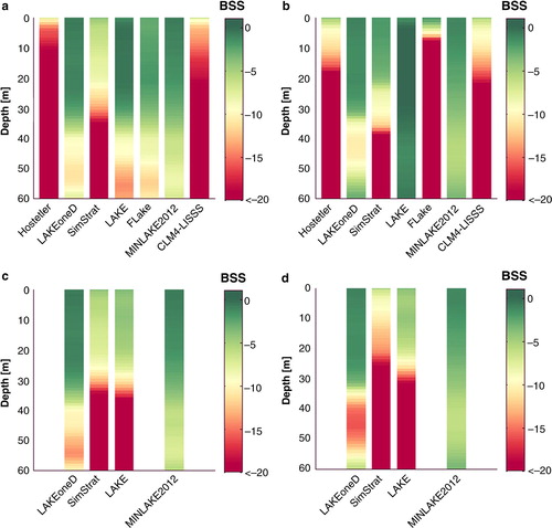
Vertical profiles of the BSS (1 m vertical increment, BSS below −20 were set to −20) indicate that models skills decrease with depth in all models (Fig. 4a). Since the BSS accounts for the effect of a systematic bias, BSS for Hostetler, CLM4-LISS and SimStrat quickly reach low values. A Taylor diagram, in contrast, allows us to assess model performance irrespective of a possible systematic bias, given its use of the normalised standard deviation σ(°C), the centred Root Mean Square Error, RMSE _c (°C), and the Pearson correlation coefficient, r. Here, surprisingly, the best model scores at 5 m are attained by CLM4-LISSS (σ _norm =0.98; RMSE _c =0.36°C; r=0.76), SimStrat (σ _norm =1.11; RMSE _c =0.39°C) and Hostetler (r=0.78) (Fig. 5a). Also at 30 and 60 m, all three models depict high skills: at these depths they are only outperformed by MINLAKE2012 in terms of σ _norm and RMSE _c (Fig. 5b–c). Hence, although Hostetler and SimStrat both depict a cold bias, they most successfully reproduce seasonal and interannual lake water temperature variability. On the other hand, towards deeper layers both LAKE and, to a lesser extent, FLake depict reducing skill compared to other models (Fig. 5b–c). For LAKE, the overestimation of the observed variance can probably be explained by a higher sensitivity of LAKE to wind velocity relative to other models (Fig. 2), whereas for FLake, this might be ascribed to the fully mixed conditions predicted during the 2003–2004 wet season (Fig. 1f): in both cases this increases the deep water temperature variability during the integration period (Fig. 2c).

Fig. 4 Brier Skill Score (BSS) vertical profiles at Ishungu (Lake Kivu), calculated per 1 m vertical increment over the respective integration period, for (a) the WS Kamembe 60 m, (b) the WS Bukavu 60 m, (c) the WS Kamembe 240 m and (d) the WS Bukavu 240 m integrations. Note that Hostetler, FLake and CLM4-LISSS were not applied in the 240 m depth experiment.

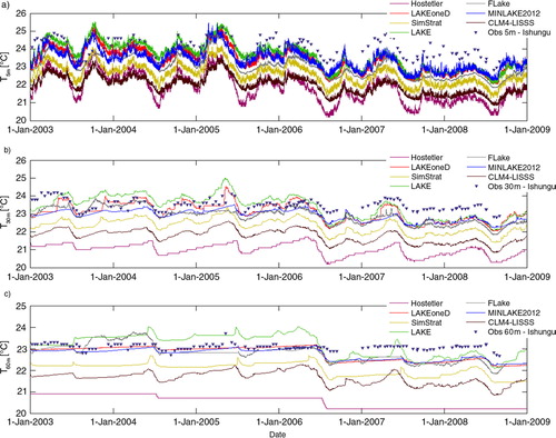
Fig. 5 Taylor diagram indicating model performance for water temperature at (a) 5 m, (b) 30 m and (c) 60 m depths at Ishungu (Lake Kivu), 2003–2008. Standard deviation σ (°C; radial distance), centred Root Mean Square Error RMSE _c (°C; distance apart) and Pearson correlation coefficient r (azimuthal position of the simulation field) were calculated from the observed temperature profile interpolated to a regular grid (1 m increment) and the corresponding modelled midday profile.

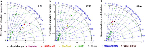
The different sensitivity experiments generally show only a small response from the models, except for FLake. This model exhibits a marked sensitivity to its configuration. Setting the light attenuation coefficient k to the highest and lowest value observed at Ishungu (WS Kamembe forcing), generally has little effect upon the different model's ability to represent water column temperatures. Vertically averaged BSS never change more than 20%, except for FLake in case of increasing k (BSS reduces by 60% as average water column temperature values cool by 0.15°C) and MINLAKE2012 when decreasing k (BSS increases by 25%). Note that when k is reduced to 0.20 m ⁻¹, BSS increases for Hostetler, LAKEoneD, FLake and MINLAKE2012.

Each control and sensitivity experiment was also conducted using meteorological measurements at Bukavu (Fig. 1) as forcing. Relative to the WS Kamembe driven control integration, vertically averaged BSS of Hostetler, LAKEoneD, SimStrat, MINLAKE2012 and CLM4-LISSS showed little to no change when forced by the alternative dataset (Fig. 4b). In contrast, LAKE enhances its predictive skill, whereas FLake's predictions deteriorate below ~5 m. For LAKE, model predictions improve especially because the observed water temperature variability at depth is well captured when forced by WS Bukavu. When LAKE is forced by WS Kamembe, significant wind velocity increases during the dry season result in too strong mixing. For FLake, the WS Bukavu driven simulation decreases in predictive skill as from mid-2004 onwards, a strong cooling of the thermocline layer sets in, reaching down to the temperature of maximum density (4°C) near the bottom. Note, however that this effect does not influence the good skill of FLake near the surface (Fig. 4a, b).

This cooling of thermocline layer in FLake has been encountered in previous studies (Subin et al., 2012b; Thiery et al., 2014) and during the development of its online version, FLake-Global (Kirillin et al., 2011). The thermal behaviour of dimictic and temperate polymictic lakes, where the average water column temperature approaches the temperature of maximum density twice or several times a year, respectively, can generally be reproduced very closely by FLake (e.g. Kirillin, 2010; Martynov et al., 2010). Lake Kivu's mixolimnion, in contrast, is characterised by a weak stratification, with a seasonally mixed layer deepening down to ~60 m, so the model needs to be able to develop and maintain this weak stratification. Possibly, the observed transition to the shallow, permanent stratification and cold bottom is related to the self-similar representation of the shape factor of the thermocline and its time rate-of-change. When the mixed layer deepens, FLake will respond by changing its thermocline shape towards a more convex shape (Mironov, 2008). However, during aforementioned cooling, the thermocline's shape factor is permanently at its maximum value, 0.8 (maximum convexity), thus inhibiting any thermocline response to mixed layer deepening. As the small-scale fluctuations of the mixed layer depth are not mirrored by changes in the thermocline shape, they could cause an unphysical loss of heat from the thermocline layer. This effect might be responsible for the observed cooling near the lake bottom which can reach down to 4°C and therewith trigger an irreversible switch to a permanently stratified mixing regime, but further research is necessary to investigate this issue.

3.2. Lake energy balance

Differences in column-integrated water temperatures between the one-dimensional lake models can be understood when comparing their lake energy budget. To this end, we first employ the relationship describing the enthalpy change H _obs of the lake's top 60 m (assuming constant pressure):

with h the water column height (60 m), ρ the lake water density (1000 kg m ⁻³), c_p the specific heat capacity of water at constant pressure (4.1813×10³ J kg ⁻¹ K ⁻¹) and the average water column temperature change computed per output time step based on the observed temperature profiles. Since all models switched off the bottom sediment routine and adopted a zero heat flux assumption at the artificial lake bottom, the predicted enthalpy change H _mod is given by:

with R _net the net radiation, and with LHF and SHF the turbulent fluxes of latent heat and sensible heat, respectively (all units W m ⁻²). Comparison of monthly average H _obs and H _mod shows that H _obs is well captured by the different models throughout most of the year (Fig. 6a). Although the observed variation is also subject to uncertainty, this given the CTD casts’ low temporal resolution and variable collection hours, the good agreement between model and observation indirectly suggests that the seasonal cycles of the radiative inputs and turbulent fluxes are correctly reproduced.

Fig. 6 Monthly average lake energy balance components (W m⁻²) at Ishungu (Lake Kivu), 2003–2008, calculated by model's surface flux routines. Components are (a) lake enthalpy change H, (b) net radiation R _net , (c) latent heat flux LHF, and (d) sensible heat flux SHF.

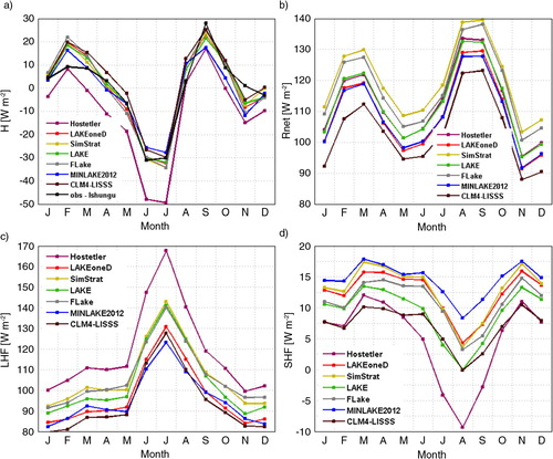
Besides variations in the computation of LHF and SHF, also different formulations are employed by the models to determine R _net , as shown in Table 3. In particular, note that FLake and CLM4-LISSS assume α _LM =0, while LAKE and LAKEoneD assume α _SM =0 for the near-infrared fraction of SW _in , on average responsible for a higher energy input into the lake of 11 W and 5 W m ⁻², respectively. Also, given the small time step used by LAKE, SimStrat and CLM4-LISSS, SW _in and LW _in require modification to achieve surface heat balance closure over each output time step. Finally, MINLAKE2012 employs the input radiative fluxes of the previous time step to compute hourly values. As a consequence of these differences, models predict variable radiative input into the lake: maximum discrepancies of monthly mean R _net values range from 13 to 20 W m ⁻² (Fig. 6b). The radiative input into the lake peaks twice a year: once during February–March and again during August–September, in agreement with the two distinct maxima in SW _net and the drop in LW _net from May to July.

In contrast to the treatment of radiative fluxes, turbulent energy exchanges show more variation among different models. For instance, relative to other participating models, in the Hostetler model, a higher portion of the available heat is consumed by evaporation: the annual mean LHF in the control integration is 14 W m ⁻² higher relative to the multi-model mean LHF (105 W m ⁻²; Fig. 6c), equivalent to an e nhanced total lake evaporation of 0.5 km³ yr ⁻¹. Over time, the resulting year-round reduction in net energy available to heat the lake will therefore enhance the cold bias observed for the Hostetler model (Fig. 6a, c), even though the enhanced evaporative cooling is partly compensated by the limited energy loss through the SHF and the higher radiative input into the lake, equivalent to 6 W m ⁻² lower and 2 W m ⁻² higher compared to multi-model means, respectively (Fig. 6d, b). For SimStrat, in turn, on the one hand slightly higher radiative input into the lake (+7 W m ⁻² relative to the multi-model mean) and on the other hand slightly positive LHF (+4 W m ⁻²) and SHF (+3 W m ⁻²) anomalies compensate for each other and gener ate a close reproduction of the observed enthalpy change, hence no change of the cold bias is expected (Fig. 6a, c, d). By analogy, also for CLM4-LISSS the cold bias is not expected to change over time (Fig. 6a). In future intercomparison experiments, wherein lake models will be interactively coupled to atmospheric models, the impact of variations in the turbulent heat fluxes on lake models will require further attention.

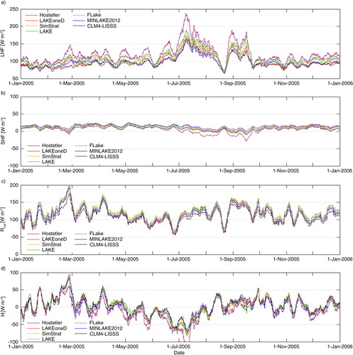
Besides differences among the models, also intra- and inter-annual variations in the water column stratification can be attributed to meteorological variability and associated changes in the lake energy balance. Since all models report high to very high correlations between wind velocity and LHF (with correlation coefficients up to 0.95 (p<0.01) in Hostetler and LAKEoneD, for instance), and because stronger winds cause enhanced mechanical mixing, variations in wind speed must certainly be considered in this case. In particular, the increasing annual mean wind velocities explain the generally reducing stratification observed throughout the integration period, as well as the sudden decrease in water temperatures observed mid 2006 (Section 3.1) and the very weak stratification during the first months of 2008 (Fig. 2a). However, variations in wind velocity provide no explanation for the high near-surface water temperatures and relatively strong stratification observed during the first months of 2005 (Fig. 2a). During this period, enhanced solar radiation reaches the lake surface, therewith increasing the amount of energy available to stratify the near-surface layers. In response to this relatively high radiative forcing (Fig. 7c), but normal turbulent heat fluxes (Fig. 7a, b) at the start of 2005, all models show similar variability in the lake's enthalpy change (Fig. 7d), and therewith reproduce the enhanced stratification during this period.

Fig. 7 Running mean lake energy balance components (W m ⁻²; 7 d averaging window) at Ishungu (Lake Kivu), for 2005. Components are (a) latent heat flux LHF, (b) sensible heat flux SHF, (c) net radiation R _net , and (d) the resulting lake enthalpy change H _.

3.3. Deep-water stratification

The deep simulations conducted by a subset of models (LAKEoneD, SimStrat, LAKE, MINLAKE2012) all succeed in reproducing Lake Kivu's meromictic state (Fig. 8). Compared to the corresponding freshwater simulation, all models display similar BSS for the top 60 m of the water column, except for LAKE, where a cold bias decreases the BSS towards 60 m (Fig. 4c). Again, it is found that setting the light extinction coefficient to the highest and lowest observed values at Ishungu, or switching off the bottom sediment routine, has little to no impact upon the results of LAKEoneD, LAKE and MINLAKE2012.

Fig. 8 Lake water temperatures (°C) at Ishungu (Lake Kivu), 2003–2008: (a) as observed, and as predicted by the models: (b) LAKEoneD, (c) SimStrat, (d), LAKE, (e) MINLAKE2012 for the 240 m deep geometry. Note that linear interpolation was applied to the observed Ishungu profiles to avoid spurious extrapolation effects, and grey areas therefore denote depths or longer time periods for which no observations are available.

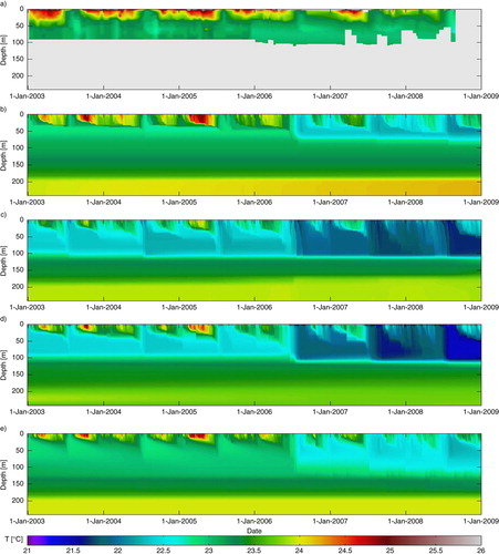
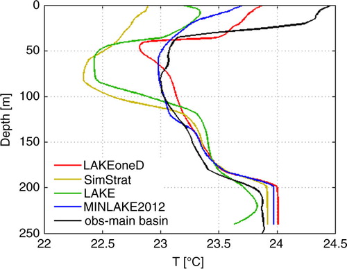
Below 60 m, modelled temperature variations are only regulated by thermal diffusion. In the permanently stratified hypolimnion represented in the deep simulations (Fig. 8), the eddy diffusivity usually vanishes and molecular diffusivity becomes the dominant term. In lake Kivu, both double diffusive convection (Schmid et al., 2010) and subsurface inflows (Schmid et al., 2005), associated with the slow upward motion of the whole water column by about 0.5 m yr ⁻¹, additionally influence the deep water temperature structure. However, none of the models involved in this study include mechanisms to account diffusivity generated by these processes. Nevertheless, the predicted temperature profiles still fairly correspond to the observed temperature profile in the main basin during February 2004 (Schmid et al., 2005), that is, 2 yr after being initialised with this profile (Fig. 9).

Fig. 9 Comparison of the observed temperature profile representative for the main basin during February 2004, as reported by Schmid et al. (2005; reproduced with permission), and corresponding modelled profiles (February 2004 average).

In the last ~50 m above ground, the heat input into the deep zone starts to influence water temperatures. At the bottom of Lake Kivu, strong geothermal heating can be expected due to its location on the East African rift. In addition to the geothermal heat flow, some warm, subaquatic springs heat the bottom layers. Together, their magnitude was estimated at 0.1–0.3 W m ⁻² by Schmid et al. (2010). The excess heat is removed both by the upward motion and enhanced diffusion through the double-diffusive staircases (Schmid and Wüest, 2012). Relative to the sensitivity experiment wherein the bottom heat flux is neglected, average temperature of the lowest 50 m is 0.02–0.18°C higher when including the bottom heat flux leads, while the water masses above this depth are almost not affected by the bottom heat flux. Throughout the integration period, LAKEoneD exhibits a warming trend of 0.24°C for the lowest 50 m, while the other comprehensive model show no temperature change for this zone.

4. Discussion

4.1. Model improvement

At this point, an interesting question is if, and in which way, the performance of individual models can be improved. For instance, for FLake, which was found sensitive both to its model configuration and forcing fields when applied to a deep, tropical lake, enhancing the robustness of the model would be beneficial. Work is currently underway to meet this need. Therewith, potentially this model will become more applicable to large, deep lakes for which no accurate forcing fields and external parameter values are available.

While for the one-dimensional lake models Hostetler, CLM4-LISSS and SimStrat, a key asset is the ability to capture the observed water temperature variability, a cold bias is observed in each case (Figs. 5, 6). However, the systematic bias can be removed through a calibration step. To illustrate the potential of a bias correction procedure, all simulations with the SimStrat model were also conducted using a modified calibration parameter for the turbulent heat fluxes. In SimStrat, the SHF and LHF are deduced from an empirical formulation which contains a parameter to calibrate the obtained result within a certain range. Through a much better reproduction of the observed lake enthalpy change, SimStrat predictions significantly improved: for instance, for the WS Kamembe driven freshwater simulation, there is now a very close agreement between modelled and observed water temperatures (Figs. 2, 10). In particular, the vertically averaged BSS increased from −23.5 to −2.9, therewith even obtaining the highest score of all models. In short, the success of the bias correction procedure illustrates the added value of a model outcome containing a systematic bias, but a correct reproduction of the observed variability, over an unbiased prediction that fails to reproduce the observed variability.

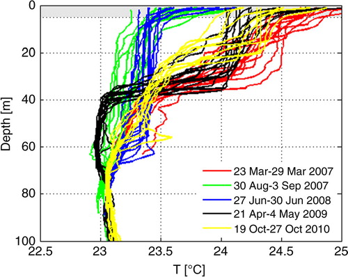
Fig. 10 Temperature profiles collected at 14 different locations in Lake Kivu during five cruises. Profiles collected at Bukavu and Kabuno bay are omitted due to their clear deviation from profiles of the main basin. Differences in the top 5 m (grey shade area) are partly due to daily variations.

4.2. Validity of the horizontal homogeneity assumption

Analysis of 60 temperature profiles collected during five cruises from March 2007 to October 2010 shows that spatial differences are clearly less important than seasonal variations (Fig. 11). Maximum horizontal temperature variations during a single cruise range from 0.3 to 0.6°C (0.5°C on average) at 5 m depth, while maximum temporal temperature fluctuations at one location range from 0.3 to 1.5°C (1.1°C on average) at 5 m. Towards 60 m, vertical temperature profiles converge, both in space and time. In agreement, previous studies report very similar thermal, chemical and biological lake characteristics across all sub-basins except Bukavu and Kabuno bay, and attribute horizontal homogeneity in the monimolimnion to long residence times (Sarmento et al., 2006; Pasche et al., 2009; Tassi et al., 2009; Pasche et al., 2011; Schmid and Wüest, 2012). The assumption of horizontal homogeneity can thus be considered valid for Lake Kivu.

Fig. 11 Lake water temperatures (°C) at Ishungu (Lake Kivu), 2003–2008, as predicted by SimStrat, using a modified turbulent heat flux calibration parameter.

5. Conclusion

The model intercomparison experiment for Lake Kivu showed that all models succeed in reproducing the timing and magnitude of water temperatures in the mixolimnion and the observed lake enthalpy change. Moreover, during the integration period the models accounting for the effects of salinity and dissolved gasses upon the water column stratification can correctly represent the meromictic state of Lake Kivu. At the same time, this study also revealed a number of strengths and weaknesses for the different groups of models.

First, while FLake is computationally the most efficient and depicts good predictive skill in the control simulation compared to other models, water temperatures towards the bottom of Lake Kivu's mixolimnion are found sensitive to modifications in the forcing fields and model configuration. Further research is needed to address the ability of FLake to represent weakly stratified lakes. However, since near-surface temperatures, in contrast to near-bottom temperatures, are more robust, the model remains a good candidate in applications where a quick and reliable computation of lake surface temperatures is important.

Second, given their limited computational expense, the Hostetler-based models (Hostetler and CLM4-LISSS) are also attractive candidates to represent lake processes within atmospheric models. Although both models predict colder water temperatures compared to observations, they correctly reproduce the observed variability, and a model calibration can potentially correct for the small systematic bias.

Third, the more comprehensive lake models, that is, MINLAKE2012 and the k-ɛ models SimStrat, LAKE and LAKEoneD, not only capture the variability of Lake Kivu's mixolimnion and therewith the effects of the meteorological controls on mixing, they also succeed in reproducing the effect of salinity and dissolved gases on the stratification. Sometimes, individual models react stronger to a certain forcing than other models, such as the heating in the lowest layers of LAKEoneD in response to the imposed geothermal heat flow (deep simulation), or the marked response to wind stress in LAKE. However, altogether, the considered comprehensive lake models are suited to investigate hydrodynamic processes occurring within large, deep lakes, and therewith make way for further studies of, for instance, biogeochemical cycling within these lakes.

Thanks to this and previous lake model intercomparison studies, the selection of a one-dimensional lake model most appropriate for a certain purpose can now be based on an informed choice. The aforementioned set of strengths and weaknesses may serve as a first indication in this respect. At the same time, this set calls for continuing the development of individual lake models, and for monitoring their progress in future intercomparison experiments.

6. Acknowledgements

We thank Martin Schmid for the helpful discussions on this project. The Institut Supérieur Pédagogique in Bukavu and Meteo Rwanda are acknowledged for supplying meteorological observations, and Alberto V. Borges for providing the temperature profiles of the CAKI cruises. We sincerely thank two anonymous Reviewers for their constructive remarks. This work was partially funded by the Research Foundation—Flanders (FWO), the Belgian Science Policy Office (BELSPO) through the research project EAGLES, and the Fund for Scientific Research (FNRS) through the research projects CAKI and MICKI, and used resources of the National Energy Research Scientific Computing Center (NERSC).

References

- Akkermans T. , Thiery W. , van Lipzig N . The regional climate impact of a realistic future deforestation scenario in the Congo Basin. J. Clim. 2014. DOI: JCLI-D-13-00361.1.
- ASTM International. Standard tables for reference solar spectral irradiances: direct normal and hemispherical on 37° tilted surface. 2012. Online at: http://www.astm.org/Standards/G173.htm .
- Balsamo G. , Salgado R. , Dutra E. , Boussetta S. , Stockdale T . On the contribution of lakes in predicting near-surface temperature in a global weather forecasting model. Tellus A. 2012; 64: 15829. DOI: 10.3402/tellusa.v64i0.15829.
- Bonan G. B . Sensitivity of a GCM Simulation to inclusion of Inland Water surfaces. J. Clim. 1995; 8: 2691–2703.
- Bonan G. B. , Oleson K. W. , Vertenstein M. , Levis S. , Zeng X. , co-authors . The land surface climatology of the community land model coupled to the NCAR community climate model. J. Clim. 2002; 15: 3123–3149.
- Borgès A. V. , Abril G. , Delille B. , Descy J.-P , Darchambeau F . Diffusive methane emissions to the atmosphere from Lake Kivu (Eastern Africa). J. Geophys. Res. 2011; 116: G03032. DOI: 10.1029/2011JG001673.
- Davin E. L. , Stoeckli R. , Jaeger E. B. , Levis S. , Seneviratne S. I . COSMO-CLM2: A new version of the COSMO-CLM model coupled to the Community Land Model. Clim. Dyn. 2011; 37: 1889–1907. DOI: 10.1007/s00382-011-1019-z.
- De Boor C . A Practical Guide to Splines. DOI: 10.1002/qj.828.
- Degens E. T. , von Herzen R. P. , Wong H.-K. , Deuser W. G. , Jannash H. W . Lake Kivu: structure, chemistry and biology of an East African Rift Lake. Geol. Rundsch. 1973; 62: 245–277. DOI: 10.1007/BF01826830.
- Descy J.-P. , Darchambeau F. , Schmid M . Descy J.-P. , Darchambeau F. , Schmid M . Lake Kivu: past and Present. Lake Kivu: Limnology and Biogeochemistry of a Tropical Great Lake . 2012; Dordrecht: Springer. 1–11.
- Fang X. , Stefan H. G . Long-term lake water temperature and ice cover simulations/measurements. Cold Reg. Sci. Technol. 1996; 24: 289–304.
- Goudsmit G.-H. , Burchard H. , Peeters F. , Wüest A . Application of k-ɛ turbulence models to enclosed basins: the role of internal seiches. J. Geophys. Res. 2002; 107: 3230–3243.
- Goyette S. , Perroud M . Interfacing a one-dimensional lake model with a single-column atmospheric model: application to the deep Lake Geneva, Switzerland. Water Resour. Res. 2012; 48: W04507. DOI: 10.1029/2011WR011223.
- Hostetler S. W. , Bates G. T. , Giorgi F . Interactive coupling of a lake thermal model with a regional climate model. J. Geophys. Res. 1993; 98: 5045–5057.
- Hostetler S. W. , Giogri F. , Bates G. T. , Bartlein P. J . Lake-atmosphere feedbacks associated with paleolakes Bonneville and Lahontan. Science. 1994; 263: 665–668.
- Jöhnk K. D . Limnophysics – Turbulenz, Meromixis, Sauerstoff. 2013; Cottbus, Germany: Institute of Limnophysics. ISBN 978-1-4475-3387-0.
- Jöhnk K. D. , Umlauf L . Modelling the metalimnetic oxygen minimum in a medium sized alpine lake. Ecol. Model. 2001; 136: 67–80.
- Kirillin G . Modelling the impact of global warming on water temperature and seasonal mixing regimes in small temperature lakes. Boreal Environ. Res. 2010; 15: 279–293.
- Kirillin G. , Hochschild J. , Mironov D. , Terzhevik A. , Golosov S. , co-authors . FLake-Global: online lake model with worldwide coverage. Environ. Model. Software. 2011; 26: 683–684. DOI: 10.1016/j.envsoft.2010.12.004.
- Kourzeneva E. V. , Samuelsson P. , Ganbat G. , Mironov D . Implementation of Lake Model FLake in HIRLAM. HIRLAM Newsletter. 2008; 54: 54–61.
- Lahmeyer and Osae. Bathymetric survey of Lake Kivu – Final report. 1998; Kigali: Republic of Rwanda, Ministry of Public Work, Directory of Energy and Hydrocarbons. 18.
- Lauwaet D. , van Lipzig N. P. M. , Van Weverberg K. , De Ridder K. , Goyens C . The precipitation response to the desiccation of Lake Chad. Q. J. Roy. Meteorol. Soc. 2011; 138: 707–719. DOI: 10.1002/qj.942.
- Lekvam K. , Bishnoi P. R . Dissolution of methane in water at low temperatures and intermediate pressures. Fluid Phase Equil. 1997; 131: 297–309.
- Lorke A. , Tietze K. , Halbwachs M. , Wüest A . Response of Lake Kivu to lava inflow and climate warming. Limnol. Oceanogr. 2004; 49: 778–783.
- Martynov A. , Sushama L. , Laprise R . Simulation of temperate freezing lakes by one-dimensional lake models: performance assessment for interactive coupling with regional climate models. Boreal Environ. Res. 2010; 15: 143–164.
- Martynov A. , Sushama L. , Laprise R. , Winger K. , Dugas B . Interactive Lakes in the Canadian Regional Climate Model, version 5: the role of lakes in the regional climate of North America. Tellus A. 2012; 64: 16226. DOI: 10.3402/tellusa.v64i0.16226.
- Mironov D . Parameterization of Lakes in Numerical Weather Prediction: Description of a Lake Model. COSMO Technical Report No. 11. 2008; 47.
- Mironov D. , Heise E. , Kourzeneva E. , Ritter B. , Schneider N , co-authors . Implementation of the lake parameterisation scheme FLake into the numerical weather prediction model COSMO. Boreal Environ. Res. 2010; 15: 218–230.
- Nash J. E. , Sutcliffe J. V . River flow forecasting through conceptual models part I – a discussion of principles. J. Hydrol. 1970; 10: 282–290.
- Ohsumi T. , Nakashiki N. , Shitashima K. , Hirama K . Density change of water due to dissolution of carbon dioxide and near-field behaviour of CO2 from a source on deep-sea floor. Energ. Convers. Manag. 1992; 33: 685–690.
- Pasche N. , Dinkel C. , Müller B. , Schmid M. , Wüest A. , co-authors . Physical and biogeochemical limits to internal nutrient loading of meromictic Lake Kivu. Limnol. Oceanogr. 2009; 54: 1863–1873.
- Pasche N. , Schmid M. , Vazquez F. , Schubert C. J. , Wüest A. , co-authors . Methane sources and sinks in Lake Kivu. J. Geophys. Res. 2011; 116: G03006. DOI: 10.1029/2011JG001690.
- Perroud M. , Goyette S. , Martynov A. , Beniston M. , Anneville O . Simulation of multiannual thermal profiles in deep Lake Geneva: a comparison of one-dimensional lake models. Limnol. Oceanogr. 2009; 54: 1574–1594.
- Poole H. H. , Atkins W. R. G . Photo-electric Measurements of Submarine Illumination throughout the Year. J. Mar. Biol. Assoc. UK. 1929; 16: 297–324.
- Sarmento H. , Isumbishu M. , Descy J.-P . Phytoplankton ecology of Lake Kivu (eastern Africa). J. Plankton Res. 2006; 28: 815–829. DOI: 10.1029/2004GC000892.
- Savijärvi H . Diurnal winds around Lake Tanganyika. Q. J. Roy. Meteorol. Soc. 1997; 123: 901–918.
- Schmid A. , Wüest A . Descy J.-P. , Darchambeau F. , Schmid M . Stratification, mixing and transport processes in Lake Kivu. Lake Kivu: Limnology and Biogeochemistry of a Tropical Great Lake Descy. 2012; Dordrecht: Springer. 13–29.
- Schmid M. , Busbridge M. , Wüest A . Double-diffusive convection in Lake Kivu. Limnol. Oceanogr. 2010; 55: 225–238.
- Schmid M. , Halbwachs M. , Wehrli B. , Wüest A . Weak mixing in Lake Kivu: new insights indicate increasing risk of uncontrolled gas eruption. Geochem. Geophys. Geosy. 2005; 6: 1–11. DOI: 10.1029/2004GC000892.
- Schmid M. , Tietze K. , Halbwachs M. , Lorke A. , McGinnis D. , co-authors . How hazardous is the gas accumulation in Lake Kivu? Arguments for a risk assessment in light of the Nyiragongo Volcano eruption of 2002. Acta Vulcanol. 2004; 14/15: 115–121.
- Song Y. , Semazzi F. H. M. , Xie L. , Ogallo L. J . A coupled regional climate model for the Lake Victoria Basin of East Africa. Int. J. Climatol. 2004; 24: 57–75.
- Spigel R. H. , Coulter G. W . Johnson T. C. , Odada E . Comparison of hydrology and physical limnology of the East African Great Lakes: Tanganyika, Malawi, Victoria, Kivu and Turkana (with references to some North American Great Lakes). The Limnology, Climatology and Paleoclimatology of the East African Lakes. 1996; Amsterdam: Gordon and Breach Publishers. 103–140.
- Stepanenko V. M. , Goyette S. , Martynov A. , Perroud M. , Fang X. , co-authors . First steps of a Lake Model Intercomparison Project: LakeMIP. Boreal Environ. Res. 2010; 15: 191–202.
- Stepanenko V. M. , Jöhnk K. , Machulskaya E. , Mironov D. , Perroud D. , co-authors . Simulation of surface energy fluxes and stratification of a small boreal lake by a set of one-dimensional models. Tellus A. 2013; 66: 1–18. (in review).
- Stepanenko V. M. , Lykosov V. N . Numerical simulation of heat and moisture transport in the “lake–soil” system. Russ. Meteorol. Hydrol. 2005; 3: 95–104.
- Stepanenko V. M. , Martynov A. , Jöhnk K. D. , Subin Z. M. , Perroud M. , co-authors . A one-dimensional model intercomparison study of thermal regime of a shallow turbid midlatitude lake. Geosci. Model Dev. 2012; 6: 1337–1352. DOI: 10.5194/gmd-6-1337-2013.
- Subin Z. M. , Murphy L. N. , Li F. , Bonfils C. , Riley W. J . Boreal lakes moderate seasonal and diurnal temperature variation and perturb atmospheric circulation: analyses in the Community Earth System Model 1 (CESM1). Tellus A. 2012a; 64: 15639. DOI: 10.3402/tellusa.v64i0.15639.
- Subin Z. M. , Riley W. J. , Mironov D . An improved lake model for climate simulations: model structure, evaluation and sensitivity analyses in CESM1. J. Adv. Mod. Earth Sys. 2012b; 4: M02001. DOI: 10.1029/2011MS000072.
- Tassi F. , Vaselli O. , Tedesco D. , Montegrossi G. , Darrah T. , co-authors . Water and gas chemistry at Lake Kivu (DRC): geochemical evidence of vertical and horizontal heterogeneities in a multibasin structure. Geochem. Geophys. Geosy. 2009; 10 DOI: 10.1029/2008GC002191.
- Taylor K. E . Summarizing multiple aspects of model performance in a single diagram. J. Geophys. Res. 2001; 106: 7183–7192. DOI: 10.1029/2000JD900719.
- Thiery W. , Martynov A. , Darchambeau F. , Descy J.-P. , Plisnier P.-D. , co-authors . Understanding the performance of the FLake model over two African Great Lakes. Geosci. Model Dev. 2014. in press.
- Verburg P. , Antenucci J. P . Persistent unstable atmospheric boundary layer enhances sensible and latent heat loss in a tropical great lake: lake Tanganyika. J. Geophys. Res. 2010; 115: D11109. DOI: 10.1029/2009JD012839.
- Verburg P. , Hecky R. E . Wind patterns, evaporation and related physical variables in lake Tanganyika, East-Africa. J. Great Lakes Res. 2003; 29: 48–61.
- Wilks D. S . Statistical Methods in Atmospheric Sciences.
- Wüest A. , Jare L. , Bürgmann H. , Pasche N. , Schmid M . Descy J.-P. , Darchambeau F. , Schmid M . Methane formation and Future Extraction in Lake Kivu. Lake Kivu: Limnology and Biogeochemistry of a Tropical Great Lake. 2012; Dordrecht: Springer. 165–180.
- Wüest A. , Piepke G. , Halfman J. D . Johnson T. C. , Odada E. O . Combined effects of dissolved solids and temperature on the density stratification of lake Malawi. The Limnology, Climatology and Paleoclimatology of the East-African Lakes. 1996; Toronto: Gordon and Breach. 183–202.