Impact of satellite-based lake surface observations on the initial state of HIRLAM. Part II: Analysis of lake surface temperature and ice cover

Abstract

This paper presents results from a study on the impact of remote-sensing Lake Surface Water Temperature (LSWT) observations in the analysis of lake surface state of a numerical weather prediction (NWP) model. Data assimilation experiments were performed with the High Resolution Limited Area Model (HIRLAM), a three-dimensional operational NWP model. Selected thermal remote-sensing LSWT observations provided by the Moderate Resolution Imaging Spectroradiometer (MODIS) and Advanced Along-Track Scanning Radiometer (AATSR) sensors onboard the Terra/Aqua and ENVISAT satellites, respectively, were included into the assimilation. The domain of our experiments, which focussed on two winters (2010–2011 and 2011–2012), covered northern Europe. Validation of the resulting objective analyses against independent observations demonstrated that the description of the lake surface state can be improved by the introduction of space-borne LSWT observations, compared to the result of pure prognostic parameterisations or assimilation of the available limited number of in-situ lake temperature observations. Further development of the data assimilation methods and solving of several practical issues are necessary in order to fully benefit from the space-borne observations of lake surface state for the improvement of the operational weather forecast. This paper is the second part of a series of two papers aimed at improving the objective analysis of lake temperature and ice conditions in HIRLAM.

• Optimal Interpolation
• data assimilation
• Lake Surface Water Temperature
• satellite observations
• lake ice cover
• numerical weather prediction
• MODIS
• AATSR

1. Introduction

The importance of a correct description of the lake surface state in climate (Duguay et al., 2006; Brown and Duguay, 2010; Krinner and Boike, 2010; Samuelsson et al., 2010; Ngai et al., 2013) and weather prediction (Niziol, 1987; Niziol et al., 1995; Zhao et al., 2012) is well known. Particularly during freezing and melting of lakes, the surface radiative and conductive properties as well as latent and sensible heat released from lakes to the atmosphere change dramatically leading to a completely different surface energy balance. Recent studies (Eerola et al., 2010; Rontu et al., 2012) have demonstrated the possibility of improving the description of the lake surface state in a numerical weather prediction (NWP) model by replacing climatological information with the objective analysis of observations. A good background for the analysis provided by the prognostic parameterisation of lake temperatures using the Freshwater Lake model (FLake) (Mironov, 2008; Mironov et al., 2010) was also shown to be important. In fact, lake parameterisations alone seem to lead to (locally) improved NWP results even without the introduction of Lake Surface Water Temperature (LSWT) observations (Eerola et al., 2010; Rontu et al., 2012).

However, the application of thermodynamic lake parameterisations in NWP has its limitations. A prognostic lake parameterisation encounters difficulties over lakes with poorly defined properties due to the complex geometry or complex topography around the lake. These are often poorly resolved by the NWP model, even if the parameterisations are able to treat the lake physical processes correctly (Semmler et al., 2012; Manrique-Suñén et al., 2013; Yang et al., 2013). The thermodynamic lake parameterisations work independently under each grid box (column), thus not taking into account horizontal exchange on or in the lakes. Thus, they are not able to handle, for example, the small-scale inhomogeneity or drifting ice on the large lakes. Objective analysis of remote-sensing observations could help the NWP model to treat the horizontal variability over lakes.

A possibly improved description of the initial state of the lakes is expected to lead to an improved weather forecast, if there is a real connection between the analysed (based on observations) and predicted (seen by the atmospheric model) state of lakes. However, in present NWP models, a prognostic lake temperature parameterisation is applied independently from the analysis (Rontu et al., 2012). To our knowledge, results of the first studies aimed at bridging the gap between the analysed and predicted state of lakes in NWP models by using the methods of Extended Kalman Filter (Ekaterina Kurzeneva, personal communication) and nudging (Mironov, 2012, personal communication), have been only recently reported (e.g. in the third workshop on ‘Parameterization of Lakes in NWP and Climate Modelling’, http://netfam.fmi.fi/Lake12). Application of these methods requires, in addition to a good thermodynamic lake parameterisation, that the observations on lake surface state are first interpolated to the NWP model grid. Hence, the objective analysis of LSWT is their starting point.

The aim of this paper is to determine if the inclusion of remote-sensing observations on LSWT can improve the analysis of lake surface state in a NWP model, compared to the description based on the thermodynamic lake parameterisation alone. By the analysed lake surface state (analysis, objective analysis), we mean here the description of LSWT and fractional ice cover over lakes at the time when each forecast cycle by the NWP model starts. This analysis results from application of a spatialisation method such as Optimal Interpolation [OI; based on Gandin (1965)] to the observed variables over lakes. We report results from data assimilation experiments performed with the three-dimensional NWP model HIRLAM (HIgh Resolution Limited Area Model), (Undén et al., 2002; Eerola, 2013) run over a northern European domain for two winters (2010–2011 and 2011–2012). Our main attention is placed on the objective analysis of the lake surface state in winter-time conditions, over freezing and melting lakes.

Our experiments focus on the use of remote-sensing observations on lakes (>6 km²) and the ways they can be introduced in the analysis. The influence of larger lakes on weather is expected to be larger than that of a multitude of smaller lakes. On the smaller lakes, there are less space-borne observations available because the number of pixels representative of pure open water or ice is limited by the surrounding land (i.e. by the within-pixel land surface contamination). We included in the HIRLAM analysis archived Moderate Resolution Imaging Spectroradiometer (MODIS) and Advanced Along-Track Scanning Radiometer (AATSR) LSWT observations, provided by the Terra/Aqua and ENVISAT satellites, and also used MERIS ice cover observations from ENVISAT for evaluation. We compared the result of pure prognostic parameterisations to the analysis based on in-situ and space-borne LSWT observations. For validation, we used additional independent satellite observations of LSWT and lake ice cover, as well as in-situ visual observations of freeze-up and break-up dates of selected lakes. We discuss in detail the maps and time-series of observed, analysed and predicted LSWT and fractional ice cover, obtained in the different experiments, in order to understand the differences and sensitivities. In the conclusions and outlook section, we discuss the perspectives and practical aspects of further usage of space-borne lake observations in operational NWP.

This is the second part of our paper on improving the objective analysis of lake surface state in HIRLAM. The first part (Kheyrollah Pour et al., 2014) (from here onward referred to as Part I) documents the processing and evaluation of remote-sensing observations applied herein for the LSWT analysis. Our study is an extension of the work reported by Eerola et al. (2010) and Rontu et al. (2012). The main differences compared to these earlier studies lie in the extended usage of remote-sensing observations and exclusion of climatological data in the analysis.

2. Observations

In this study, in-situ and remote-sensing observations on lake surface state are introduced into the surface data assimilation system and used for comparison and validation. Table 1 summarises the different observation types and their usage, discussed in this section.

Table 1. Summary of observations used in this study

Variable	Source of observation	Spatial coverage	Temporal coverage	Usage
LSWT	MODIS (1 km^2)	70 pixels (41 lakes)	2010.11.01–2012.05.31	Objective analysis
LSWT	AATSR (1 km^2)	15 pixels (Lake Ladoga)	April 2011	Objective analysis
LSWT	FMI Marine Services^a	Swedish lakes^a,b	Oct.–May, 2010–2012	Objective analysis
Lake water temperature	SYKE measured	27 Finnish lakes	2010.11.01–2012.05.31	Objective analysis
Freeze-up/break-up dates	SYKE visual observation	27 Finnish lakes	2010.11.01–2012.05.31	Evaluation
Ice fraction	MERIS (300 m^2)	Lake Ladoga	April 2011	Evaluation

^aFMI Marine Services=partly manual interpolation of remote-sensing and ship observations on SST and properties of ice cover.

^bSwedish lakes=Vänern, Vättern and Mälaren.

2.1. Satellite LSWT observations

Satellite thermal infrared sensors offer a global coverage and high temporal resolution of lake temperature observations (Part I). This represents a significant advantage over in-situ observing systems that provide point measurements, often only close to the shoreline. In the present study, 70 predefined pixels were selected over 41 northern lakes (Fig. 1, large image, black dots). The selection of a limited number of pixels, instead of using all available 1 km×1 km resolution data, is a limitation which was dictated by practical reasons, and will be discussed in the concluding section. The satellite observations were used at the nearest analysis time within ±3 h when available, i.e. under cloud-free conditions over each pixel location. A detailed description of the satellite observations and of the algorithms applied for extraction and screening can be found in Part I, only a short summary is given here.

Fig. 1 (a) Location of the MODIS pixels over the northern lakes. Independent lakes are marked with orange dots. (b) Location of 27 lakes (dark blue polygons) with SYKE measurement sites in Finland. (c) Detailed view of the selected MODIS and AATSR pixels over the lakes Ladoga (left) and Onega (right).

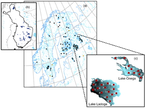
LSWT data were derived from the MODIS sensor, which operates on NASA's Terra and Aqua Earth Observation System (EOS) satellites (http://modis.gsfc.nasa.gov). The LSWT level 3 data, referred to as UW-L3 here onwards, were generated at the University of Waterloo. These data were evaluated using ground measurements over lakes in the same study area during the open-water season (Part I) and over two large Canadian lakes (Kheyrollah Pour et al., 2012). For MODIS observations, both daytime and nighttime Terra and Aqua LSWT observations were selected in order to maximise the amount of available input data to the analysis. Data from the AATSR, onboard the European Space Agency (ESA) ENVISAT satellite, were extracted over Lake Ladoga for the same 15 pixels as for MODIS (Fig. 1, Lake Ladoga image, red squares). Aqua and Terra satellites passed over our study area daily around 08–10 UTC and 20–01 UTC. AATSR observations were available 06–08 UTC every third day in April 2011.

2.2. In-situ lake water temperature observations

Regular in-situ lake water temperature measurements are provided by the Finnish Environment Institute (Suomen Ympäristökeskus, SYKE). SYKE operates 32 regular lake and river water temperature measurement sites in Finland. The temperature of the lake water is measured every morning at 8.00 AM local time, close to shore, at 20 cm below the water surface. The measurements are either recorded automatically (13 stations) or manually and are performed only during the ice-free season (Rontu et al., 2012). Measurements from 27 lakes (Fig. 1, upper left map), which are also used by the FMI operational HIRLAM, were included in all experiments reported in this study.

The operational Baltic Sea ice chart (Grönvall and Seinä, 2002) produced by FMI's Marine Service also provides manually processed, satellite-based observations of water temperature and ice properties over Swedish lakes Vänern, Vättern and Mälaren. From these, pseudo-observations of LSWT have been derived since 10 January 2011 for the FMI operational HIRLAM at a few selected pixels in winter season approximately between 15 October and 15 May each year. In this derivation, ice fractions are converted to LSWT and ice-flag temperatures by applying the inverse of the method described in Section 3.3. These data were included in the present experiments when available, but their influence is not discussed herein.

2.3. Data for comparison and validation

Historical freeze-up and break-up dates from SYKE for most of the 27 Finnish lakes (Fig. 1) were used for comparison with MODIS observations and HIRLAM analysis results. These freeze-up and break-up dates are based on visual observations from shore and represent the complete freezing and melting in small lakes. For the large lakes, separate freeze-up and break-up dates for the central open waters and coastal areas may be given by SYKE. Among the lakes discussed in this study, this is the case only for Lake Inari, where we used central open-water dates. The visual observations are made independently of the water temperature measurements. These observations are made over a larger number of lakes in Finland than was used here, thus available for further studies.

MODIS UW-L3 LSWT observations were prepared but withheld from the HIRLAM analysis, in order to be used as independent data for comparison over Lakes Bolmen and Hjälmaren in Sweden and Lakes Valday and Kuito in Russia (orange dots in Fig. 1, coordinates shown in Table 3). MERIS-derived ice fraction observations for Lake Ladoga were utilised in this study for the month of April 2011. The ice fraction data were produced by the Norwegian Computer Center as part of the ESA North Hydrology project (http://env-ic3-vw2k8.uwaterloo.ca:8080). MERIS was a core instrument of ESA's ENVISAT satellite platform that operated between March 2002 and April 2012.

3. Analysis of lake surface state

Over water bodies in HIRLAM surface water temperature observations are treated with OI (Gandin, 1965). The methods of OI analysis of LSWT are based on those applied for sea surface temperature (SST). We summarise the method briefly here, and present our findings concerning the needs of its further development in the conclusions.

3.1. OI of LSWT

OI analysis, integrated into the framework of HIRLAM, is applied for SST (Undén et al., 2002). More recently, the same method has been extended for the analysis of LSWT (Eerola et al., 2010; Rontu et al., 2012). In the near-surface analysis of HIRLAM, OI is applied to spread the information from irregularly located observations to regularly located grid points for the initialisation of the next forecast cycle. This is done by correcting the background field with observations. For lakes, the background can be provided either by the previous analysis or by a short forecast. In the latter case, the background LSWT is derived from the surface temperature forecast by the lake model (FLake), which is incorporated in HIRLAM as a parameterisation scheme. Here, the evolving three-dimensional state of the atmosphere also influences the predicted state of lakes and hence the background for the LSWT analysis. A good background is especially important over lakes where observations are sparse or not available at all.

The analysis at a grid point k is determined by a linear combination of the observed departures from the background1

where a _k is the analysis, b _k the background and w _ki are the weights given to observations i=1,…,N, y _i the observations and b _i the background values interpolated to the observation points.

Derivation of the weights relies on the assumption that observation and background errors are uncorrelated. In OI, the weights w _ki in eq. (1) are determined by inverting a matrix which represents the background and observation error covariances (Daley, 1991). For the SST and LSWT analysis applied in HIRLAM, the background error covariance, which to a large extent determines the resulting analysis, is treated by modelling the autocorrelation and standard deviation of the background error separately. A Gaussian autocorrelation function is applied, which depends on distance2

where g(r) is the autocorrelation function, r is the distance and L _H is a horizontal length scale (L _H =80 km). So g(r) depends only on distance between the points. The observation and background error variances, which enter the diagonal of the matrix, are assigned prescribed constant values (we assumed a standard deviation error 1.5°C for observations and 1°C for background).

The OI analysis integrated into the NWP model differs from the stand-alone analysis approach, as applied for SST and LSWT [e.g. by the Operational Sea surface Temperature and sea and lake Ice Analysis (OSTIA) (Donlon et al., 2012; Fiedler et al., 2014)] in two essential aspects. In OSTIA, the background is always provided by the previous analysis done (e.g. on the previous day), and relaxed towards the LSWT climatology, which is taken from ARC-lake database (Hook et al., 2012; MacCallum and Merchant, 2012). If the observations are missing for a long time or not available at all over some lakes, climatology gets a large weight. In the case of OSTIA, realistic lake climatology is available over lakes of the ARC-lake database (ca. 250 lakes worldwide, around 15 over our present study area). More importantly, no climatology is able to represent the current and near past atmospheric conditions, which basically determine the current lake temperatures. In our case, it is also possible to use previous analysis as the background and relax to climatology at each HIRLAM grid box, where a fraction of lake is detected. However, in our case, this is even more problematic, because our LSWT climatology was extrapolated to any lake from SST climatology not lake climatology, which is unrealistic. This is why we prefer the background provided by the prognostic lake parameterisation, calculated within HIRLAM for each time step at each grid box which contains a lake fraction.

Another point is that our OI method works also across the lakes, sometimes interpolating LSWT observations from nearby lakes if these are close enough to influence. Thus, an analysed LSWT value is always available in every lake grid point of HIRLAM. In this respect, we are again not limited by the choice of pre-selected large lakes, between which OSTIA can also interpolate. In HIRLAM, special care is taken not to mix sea and lake observations in the analysis near the sea coast. However, to fully benefit from the across-lake interpolation possibility, it will be necessary to derive autocorrelation (structure) functions, depending not only on the horizontal distance but also at least on the depth and possibly on the elevation differences within and between the lakes.

3.2. Quality control

In HIRLAM, quality control (QC) of the observations is performed prior to the actual analysis. QC is done in two consequent phases: first the observations are tested against the background, then each observation is compared to the surrounding observations. For the background check, a normalised difference Δ _i between the observed value and the background value interpolated to the observation point is calculated as3

where σ _b and σ _o denote the background and observation error standard deviations. If Δ _i is larger than a prescribed threshold value, the observation is rejected by the background check. The check against surrounding observations first excludes the observation to be checked, and then performs OI analysis to this point by using the nearby observations. The difference between the analysed and the observed value, again normalised by the observation and background error standard deviations, is tested against a prescribed threshold value. It is difficult to choose optimal criteria for this threshold. In order to retain a maximum number of observations, a quite liberal approach was adopted here: the threshold was set so that only those LSWT observations which deviated from the background by more than 10°C were rejected [eq. (3)].

3.3. Treatment of ice fraction

In HIRLAM, a diagnostic ice fraction is derived from the analysed LSWT. Thus, neither space-borne nor in-situ ice concentration, ice thickness and ice temperature observations are directly analysed. The diagnostic ice fraction is estimated in a simple way: we assume that a lake grid square is fully ice-covered when LSWT falls below −0.5°C and fully ice-free when LSWT is above 0°C. Between these temperature thresholds, the fraction of ice changes linearly. A range from −0.5 to 0°C has been chosen to account for the variability and uncertainty of the analysed LSWT within the model resolution. A corresponding ice-flag value of −0.6°C was assigned to LSWT while creating the background to LSWT analysis in such grid squares, where the ice thickness predicted by FLake exceeded a threshold value of 1 mm. An observation ice-flag value of −1.2°C was assigned to all MODIS surface temperature values below −0.5°C over lakes. These were assumed to represent full ice cover in their surroundings. In the case of SYKE observations, the ice-flag value was given to all measurements showing 0°C water temperature. If we had instead assigned LSWT observations a missing value under the observed ice, we would have excluded from the analysis all observations representing ice conditions, thus letting the background (FLake or previous analysis) alone to determine. In the melting and freezing conditions, removal of all information about ice would give more weight to the water observations and most probably lead to incorrect spread of open-water information into the nearby ice-covered part of the lake.

This kind of procedure, which was inherited from the SST analysis and sea ice diagnostics, represents a simplified but non-physical way of handling ice concentration. Here a single variable, namely LSWT, is taken to represent in the analysis both itself, i.e. the water temperature, and another variable, ice cover. This is why the LSWT flag values enter the OI analysis and QC together with the real observations. However, the choice of the ice concentration versus LSWT range and the flag values is rather arbitrary. The sensitivity of the resulting LSWT and ice cover to these choices should be systematically studied. The eventual solution of the problem could be found in assimilation of the observed and predicted physical properties of ice, such as ice thickness (see Section 6 for discussion).

4. Description of the analysis-forecast system and setup of experiments

All our experiments were run in the framework of HIRLAM version 7.4 (www.hirlam.org). This HIRLAM version incorporates fully integrated FLake model, applied as a parameterisation scheme for prediction of lake water, ice and snow temperatures and ice thickness and snow depth over lakes (Rontu et al., 2012). We used a model setup with a horizontal resolution of 6.8 km over a northern Europe experimental domain (Fig. 1) with 65 levels in vertical between the surface and the 10 hPa level in the atmosphere. Four data assimilation-forecast cycles were run every day, starting at 00, 06, 12 and 18 UTC. For the upper-air data assimilation, a three-dimensional variational method was used. The lateral boundary conditions for the atmospheric model were provided by the fields of the European Centre for Medium-Range Weather Forecasts (ECMWF) analysis.

Three initial sets of experiments were designed to study the impact of assimilated remote-sensing LSWT observations over the major northern European lakes (Table 2). In the baseline experiment TRULAK (SYKE water temperature observations, FLake parameterisations), the prognostic lake parameterisations inside the forecast model provided the background for the LSWT analysis. This follows the setup of the reference HIRLAM used for the FMI operational NWP. No satellite observations were used in the baseline experiment, just SYKE in-situ water temperature measurements over Finland. In the second experiment, called NHFLAK (SYKE water temperature and MODIS LSWT observations, FLake parameterisations), remote-sensing LSWT observations were also included. In the last experiment, referred to as NHALAK (SYKE water temperature and MODIS LSWT observations), LSWT observations were used to correct the background provided by the previous analysis, which was relaxed towards ‘ocean-derived’ LSWT climatology of the reference HIRLAM (Rontu et al., 2012). AATSR observations over Lake Ladoga only were included in two additional short experiments, called NHALAA (AATSR LSWT observations) and NHFLAA (AATSR LSWT observations, FLake parameterisations), run for April 2011. SYKE in-situ water temperature observations from the Finnish lakes were included in all experiments.

Table 2. Definition of the HIRLAM experiments

Experiment	Period	Observations	Background
TRULAK	2010.11.01–2012.05.31	SYKE^a	FLake+6 h^c
NHFLAK	2010.11.01–2012.05.31	SYKE^a+MODIS^b	FLake+6 h^c
NHALAK	2012.01.01–2012.05.31	SYKE^a+MODIS^b	previous analysis
NHFLAA	2011.04.01–2011.04.30	SYKE^a+AATSR^d	FLake+6 h^c
NHALAA	2011.04.01–2011.04.30	SYKE^a+AATSR^d	Previous analysis

^aSYKE=Measured LSWT over 27 lakes in Finland.

^bMODIS=MODIS observations in 70 pixels.

^cFLake+6 h=Freshwater Lake model parameterisations within HIRLAM, 6 h forecast.

^dAATSR=AATSR observations over Lake Ladoga only.

For the lake analysis and parameterisations, information about the lake depth and fraction of lake in each grid box is needed. Lake depths were obtained from the lake data base for NWP and climate models (Kourzeneva et al., 2012a). Fraction of lakes was taken from the HIRLAM physiography description (Undén et al., 2002). The lake fraction was originally derived for HIRLAM using the 1-km resolution Global Land Cover Characteristics (GLCC) data base (Loveland et al., 2000). For the very first cycle, prognostic inside-lake variables were initialised with gridded lake climatology (Kourzeneva et al., 2012b). The very first LSWT analysis was replaced by the reference HIRLAM LSWT climatology when starting each of the experiment series. Note that these two climatologies are different – the first is the climatology of FLake prognostic variables, the second has been extrapolated from SST for LSWT analysis only.

5. Results and discussion

5.1. Freeze-up and break-up dates

Freeze-up and break-up dates interpreted from SYKE, MODIS and MERIS observations were compared with the dates given by HIRLAM experiments for selected representative lakes (Table 3). Lake Lappajärvi is a regular-form, medium-size and relatively shallow lake located in western Finland. SYKE water temperature measurements are available for this lake. Lakes Bolmen, Hjälmaren, Valday and Kuito whose MODIS observations were excluded from HIRLAM analysis, resemble Lake Lappajärvi. Lake Inari in the Finnish Lapland is large, with islands, a complex coastline and bathymetry, and is also represented in HIRLAM analysis by SYKE water temperature observations. Over the large, deep and open Lakes Ladoga and Vänern the break-up and freeze-up processes progress differently than over smaller lakes: ice forms, cracks and drifts depending on the wind speed and direction. However, for simplicity, only one point is chosen to illustrate the surface state of these lakes here. Coordinates of the chosen locations and the mean depth of lakes are shown Table 3. A few preliminary remarks related to the accuracy of the dates are necessary before discussion:

• SYKE freeze-up and break-up dates: These dates are based on visual ground-based observations, which are independent of the SYKE water temperature measurements used by the HIRLAM analysis.

• MODIS dates: Especially during the freezing period, which is often cloudy and dark, the MODIS observations over a chosen location may be missing for several days, even weeks. During the freezing and melting periods, MODIS LSWT may oscillate from one measurement to another by several degrees, sometimes jumping to both sides of zero. Some subjective reasoning was applied when determining the dates from this information.

• HIRLAM dates: In Table 3, the dates are shown based on the OI analysis of HIRLAM, which used either the prognostic temperatures from FLake (experiments NHFLAK and TRULAK) or the previous analysis (experiment NHALAK) as background. For various reasons, the analysed temperature also has a tendency to oscillate between analysis cycles, which during the freezing and melting periods may lead to oscillation of the ice fraction. Thus, here again some subjective reasoning was needed to determine the freezing and melting dates. In some cases, a transition period up to 3 weeks is shown to indicate the uncertainty related to this oscillation.

• MERIS ice fraction: Data were prepared for comparison in 2011 for Lake Ladoga. MERIS-derived ice fraction information was obtained from pixels, each representing an area of 300 m×300 m.

Table 3. Freezing and melting dates of selected lakes given by observations (SYKE and MODIS) and analyses by experiments (TRULAK, NHALAK, NHFLAK as defined in Table 2)

Melting 2010	Freezing 2010/11	Melting 2011	Freezing 2011/12	Melting 2012
Lappajärvi, Finland	23.67E 63.14N	Mean depth 7 m
SYKE	20100504	20101122	20110503	20111231	20120502
MODIS	20100505	20101105	20110501	20111203	20120429
TRULAK	–	20101108	20110418	20111217	20120424
NHFLAK	–	20101117	20110421	20111213	20120424
NHALAK	–	–	–	–	20120429
Inari, Finland	28.10E 68.87N	Mean depth 14 m
SYKE	20100603	20101126	20110603	20111230	20120531
MODIS	20100512	20101106	20110515	20111201	20120527
TRULAK	–	Before 20101101	20110506	20111121	20120509
NHFLAK	–	20101107	20110507	20111125	20120507
NHALAK	–	–	–	–	20120526
Ladoga,^a Russia	32.50E 60.82N	Mean depth 33 m
MODIS	20100513	20110115	20110508	20120125	20120501
MERIS	–	–	20110509	–	–
TRULAK	–	20101206–20110111	20110404–16	20120123	20120401–13
NHFLAK	–	20101213–20110101	20110430	20120127	20120428
NHALAK	–	–	–	20120128	20120511
Vänern,^b Sweden	13.75E 59.15N	Mean depth 50 m
MODIS	20100410	20110206	20110409–0429	Partial ice	Partial ice
TRULAK	–	20101108	20110410–0430	Almost no ice	Almost no ice
NHFLAK	–	20101223	20110412	Almost no ice	Almost no ice
NHALAK	–	–	–	Almost no ice	Almost no ice
Bolmen, Sweden	13.69E 56.87N	Mean depth 5 m
MODIS	20100409	20101130	20110328	20120115	20120223
TRULAK	–	20101127	20110320	20120123	20120312
NHFLAK	–	20101127	20110321	20120123	20120312
NHALAK	–	–	–	20120206	20120226
Hjälmaren, Sweden	15.85E 59.24N	Mean depth 10 m
MODIS	20100418	20101121	20110414	20110108	20120326
TRULAK	–	20101108–1202	20110408	20120108–0130	20120316
NHFLAK	–	20101128	20110404	20120119	20120325
NHALAK	–	–	–	20120203	20120329
Kuito, Russia	31.42E 65.14N	Mean depth 19 m
MODIS	20100514	20101115	20110519	20111121	20120513
TRULAK	–	20101105	20110425	20111129	20120417
NHFLAK	–	20101108	20110427	20111122–29	20120417
NHALAK	–	–	–	–	20120516
Valday, Russia	33.31E 57.99N	Mean depth 14 m
MODIS	20100507	20101122	20100508	20111122	20120412
TRULAK	–	20101127	20110403	20111225	20120327
NHFLAK	–	20101202	20110404	20111225	20120329
NHALAK	–	–	–	–	20120420

^aLadoga, pixel 9, see Fig. 1 for map.

^bVänern, pixel 4.

SYKE and MODIS freeze-up and break-up dates were first compared over two Finnish lakes, Lake Lappajärvi and Lake Inari. During lake melt, SYKE and MODIS dates differed from each other by less than 10 d. During freezing, the difference could be several weeks. It is possible that the MODIS LSWT observations on selected 1 km×1 km pixels may indicate melting or freezing before the SYKE observer determines that the whole lake is unfrozen or frozen. To avoid this error, MODIS visible images (bands 7, 2 and 1) were used to make sure that the chosen pixel values represented correctly the whole lake area. The difference between SYKE and MODIS freeze-up and break-up dates, shown in Table 3 for Lake Inari and Lake Lappajärvi, was similar over the other Finnish lakes (not shown). The uncertainty of a lake melting date, derived from MODIS by a couple of weeks compared to the in-situ data could be due to the visual in-situ observation as the observer cannot monitor the whole area of the lake from the lake shoreline. The uncertainty of the freezing dates could be up to 1 month.

Over Lake Ladoga, no SYKE freeze-up and break-up dates observations were available to be compared with MODIS. Melting dates interpreted from MERIS measurements in spring 2011 over Lake Ladoga (shown for pixel 9 in Table 3, see Fig. 1 for the map), seem to agree with the dates interpreted from MODIS LSWT measurements. Thermal satellite observations from AATSR-L1B are used to develop MERIS lake ice products to detect cloud cover, therefore both MERIS ice cover and MODIS temperature observations represent the surface only under clear-sky conditions. This limits the accuracy of the dates derived from these measurements in a similar way.

The freezing dates given by the analysis of the experiment NHFLAK (FLake+MODIS LSWT+SYKE water temperature) came in general closer to the observed dates compared to the dates from experiment TRULAK (in the area of the analysis domain outside Finland, where no SYKE temperature observations are available, FLake alone was used). In spring, the analysed melting dates by both TRULAK and NHFLAK were always earlier than those indicated by MODIS observations at the selected pixels. The largest differences between melting dates interpreted from HIRLAM analysis and directly from MODIS observations were more than 1 month when the analysis was determined by the FLake background alone. This was the case for TRULAK over all lakes and NHFLAK over the independent lakes Bolmen, Hjälmaren, Kuito and Valday. Over the Finnish lakes, SYKE temperature observations were available only well after melt. Thus, during the melting period, the warm FLake background dominated over the (sparse) MODIS observations also in NHFLAK.

In cases when the inclusion of MODIS observations to NHFLAK did not change the analysed state of lakes significantly, the reasons may have been due to the fact that: 1) MODIS data were seldom or not at all available for analysis, 2) the prognostic parameterisations were good and agreed with MODIS, or 3) the difference between MODIS and FLake was so large that the observations were rejected by the QC while comparing the background and observations. Rejections were, however, uncommon in autumn and when the lakes were frozen (between the dates shown in Table 3), but became more frequent at the end of May with rising lake water temperatures after the ice melt. It is possible that the FLake background dominates in the analysis over the large lakes because the information brought by the selected MODIS pixels is simply insufficient there (see also Section 5.2).

The NHALAK experiment combined SYKE water temperature and MODIS LSWT observations with the background given by the previous analysis, which had been relaxed towards the LWST climatology. This experiment, which was run only for January–May 2012, followed the observations more closely than the prognostic experiments TRULAK and NHFLAK, but only when observations were available on the lake or close to it (i.e. when the effect of background field was small). Elsewhere, the analysis tended towards the (wrong ocean-derived) climatology, possibly resulting in a completely useless description of lake surface state [not shown in Table 3, see an example in Rontu et al. (2012)]. Over Lakes Lappajärvi and Inari, NHALAK improved the analysis so that the melting dates became closer to the SYKE temperature observation. Over Lakes Ladoga and Vänern, the dates became closer to the MODIS observations. In spring, interpretation of the point values over the large lakes may be affected by the uneven melting and drifting ice. The NHALAK melting dates over the selected lakes seem to agree with MODIS observations within about 1 week. The agreement is better than in the case of NHFLAK, whose analysis was dominated by the FLake parameterisations. Freezing dates from NHALAK were available only over a few lakes because this experiment was started in the middle of winter.

5.2. April 2011 comparison

For visual comparison of the full-resolution satellite observations with the NWP analysis during melt, MODIS (daytime and nighttime) and AATSR (morning) LSWT, as well as MERIS ice fraction on 12 April 2011 were mapped (Fig. 2) and compared with the HIRLAM analysis and background by experiments NHFLAK and NHFLAA (Fig. 3). In April, the ice cover on Lake Ladoga started to break, which makes comparison of observations and simulations both interesting and challenging due to the moving ice on the lake.

Fig. 2 Surface temperature on 12 April 2011: (a) MODIS visible image, (b) MERIS ice fraction, (c) AATSR surface temperature (between 8 and 10 AM local time), (d) MODIS daytime surface temperature (between 10 AM and 12 PM local time) and (e) MODIS nighttime (between 10 PM and 3 AM local time).

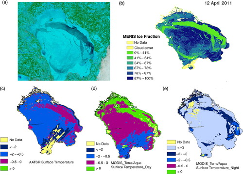
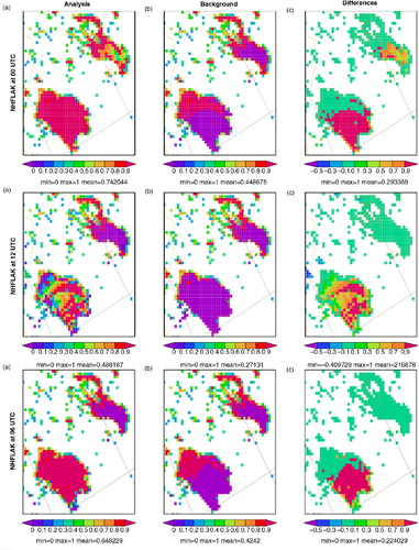
Fig. 3 HIRLAM ice fraction (0–1) on 12 April 2011, diagnosed from LSWT: (a) analysis, (b) background and (c) their differences. NHFLAK (SYKE, FLake, MODIS) at 00 UTC (upper panel) and at 12 UTC (middle panel), and NHFLAA (SYKE, MODIS) at 06 UTC (lower panel).

MERIS estimation of ice fraction (Fig. 2b) agrees well with the MODIS visible image (Fig. 2a), indicating an area consisting of a mixture of ice and water (MERIS: values between 0 and 54% ice fraction) in the northeastern part and, to a lesser extent, in the southwestern part of the lake. On the northeastern part of Ladoga, MODIS daytime observations (between 08 and 10 UTC) show temperatures just above 0°C and around 2–3°C lower at nighttime (between 20 and 01 UTC) (Fig. 2d and e). The daytime MODIS observations show warmer temperatures compared to AATSR (Fig. 2c). The AATSR observations were available earlier in the morning (06–08 UTC) than MODIS. Thus, the stronger heating of the surface by solar radiation at noon may explain the difference.

The ice fraction from HIRLAM (Fig. 3, left column) was derived from the analysis of LSWT (for the method, see Section 3.3), which was based on the combination of MODIS (experiment NHFLAK) or AATSR (experiment NHFLAA) observations (Fig. 4) and the background field by FLake. For comparison, the ice fraction diagnosed from the +6 h ice thickness forecast by FLake parametrisation is shown (Fig. 3, middle column). In this diagnosis, the lake within each grid square is assumed to be either completely ice-covered or completely ice-free, i.e. no fractional ice is assumed. Both the analysed and predicted ice patterns differ from those of the mid-day and nighttime satellite observations (Fig. 2). According to the background forecast, Lake Ladoga should have been almost ice-free during the day, while at night and in the morning the northern part seems frozen. Similarly, the analysis indicates a frozen lake at night (based on MODIS) and early morning (based on AATSR) but partially melted during the day.

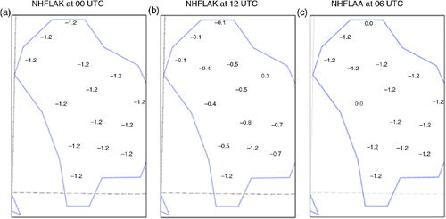
Fig. 4 LSWT observations used for HIRLAM analysis over Lake Ladoga on 12 April 2011: (a) MODIS for NHFLAK (SYKE, FLake, MODIS) at 00 UTC, (b) MODIS for NHFLAK at 12 UTC and (c) AATSR for NHFLAA (SYKE, FLake, AATSR) at 06 UTC.

Three technical comments are needed for understanding the possible reasons of the difference between the analysis and the satellite observation. First, the horizontal resolutions of the model and satellites are different: 7 km for HIRLAM (the boxes visible on the maps in Fig. 3 represent grid squares), 1 km for MODIS and AATSR, and 300 m for MERIS. Thus, we would not expect HIRLAM to represent all details of the ice cover detected by the satellites. Second, the diagnostic ice fraction of the HIRLAM analysis is derived from the analysed LSWT in a very simple ad-hoc way (Section 3.3). Consequently, all HIRLAM ice fractions are derived from temperatures between the freezing temperature and an artificially set lower limit of −0.5°C. This is not the same variable as the MERIS ice fraction, which can represent physically realistic ice properties within its 300 m×300 m pixels. In addition, the method involves unphysical ice-flag temperatures (see section 3.3), which may enter the analysis together with the real observations, thus adding uncertainty to the resulting analysis. Third, the LSWT analysis of the HIRLAM experiment NHFLAK over Ladoga is based on a selection of observed LSWT from a maximum of 15 MODIS or AATSR pixels (see Figs. 1 and 4), combined with the FLake +6 h forecast which is used as the background. This means that over Lake Ladoga, the largest part of the information from the ca. 30000 theoretically possible MODIS pixels remains unused in the analysis at the ca. 600 HIRLAM grid squares, and the result is compared to ca. 300000 MERIS pixels.

newpage pagenumber="10"/>Of the 15 possible MODIS pixels, 14 were available and accepted for the analysis at 00 UTC on 12 April (MODIS observation at 23 UTC, 11 April 2011, Fig. 4a). They all show the flag value of ice, assumed for MODIS when the observed LSWT is below −0.5°C. Twelve hours later, at 12 UTC on 12 April (MODIS observations at 9 and 11 UTC, Fig. 4b), the analysis input also included 14 observed values, the most northeastern one (pixel 8) indicating unfrozen conditions and the other temperatures slightly under the freezing point. AATSR observations assimilated at 06 UTC indicated that the northeastern (pixel 1) and western (pixel 6) areas may have been unfrozen, while the remaining 15 pixels were frozen (Fig. 4c).

AATSR observations were extracted for the chosen 15 pixels and applied for HIRLAM analysis on the 5–6 d in April 2011 when they were available. AATSR observations always represent morning conditions. An example of their influence in the experiments NHFLAA (with FLake background) and NHALAA (with previous analysis background), as compared to the influence of MODIS observations in the experiments NHFLAK (with FLake background) and NHALAK (with previous analysis background), is shown in Fig. 5 for the centre of Lake Ladoga at pixel 7 during April 2011. The background given by FLake (experiment NHFLAA) and by the previous analysis (NHALAA), which was relaxed towards climatology, was very different. FLake would indicate melting during the first week of the month, while the MODIS and AATSR observations pointed to melting during the last week. Both MODIS and AATSR provided enough observations to modify the analysis accordingly, so that the analyses indicated melting closer to the end of April. Without observations and FLake (i.e. relying on climatology only), melting would have occurred after the end of April.

Fig. 5 Analysis (red), background (black) and observation (blue) in the grid point nearest to pixel 7 over central Ladoga during April 2011 in the experiments (a) NHFLAA (SYKE, FLake, AATSR), (b) NHFLAK (SYKE, FLake, MODIS), (c) NHALAA (SYKE, AATSR) and (d) NHALAK (SYKE, MODIS). Only times when MODIS observations were available are shown. No data are rejected here.

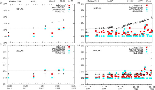
Only those days when observations were available are shown in Fig. 5. When observations are sparse, the FLake background dominates the analysis outcome. The behaviour of FLake may vary between individual grid columns because of their different lake depths. For large lakes such as Ladoga, an approximate bathymetry is available in HIRLAM (Kourzeneva et al., 2012a). However, to a large extent, the conditions over the lake remain homogeneous, also from the point of view of the atmospheric forcing. This means that the background for LSWT analysis, given by FLake, also contains little horizontal variability. In addition, the analysis at each grid point is influenced by all nearby observations, whose values and availability may vary in time. Over Lake Ladoga, these nearby observations consisted of the selected 15 pixels, each of which would have an influence to some extent over the whole lake, according to eq. (2).

The different behaviour of MODIS observations during day and night contributed to an unrealistic jumping of the HIRLAM NHFLAK analysis from frozen to unfrozen conditions: during the day unfrozen conditions prevailed, during the night the lake seemed frozen. This was typical during the melting period over Lake Ladoga, also over the other lakes (not shown). Jumping of the MODIS observations between sequential observations is confirmed by Fig. 5. AATSR may suffer less from this feature, perhaps because observations at the selected pixels were quite sparse in time but representing always the similar morning conditions. Also the lake parameterisation may contribute to the unrealistic oscillation across the freezing temperature (e.g. by absorbing solar radiation too effectively during daytime).

The reason for the difference between the cold nighttime and warm daytime MODIS lake surface temperatures remains to be understood. At night, water on ice may refreeze due to long-wave radiative cooling of the surface. In this case, the MODIS temperature would not represent that of the lake, but the temperature of the refrozen melt water on ice. One could also speculate on the possibility of the formation of fog during the night over the melting ice. This type of fog, perhaps quite impossible to distinguish from the underlying surface in the satellite image, would show colder temperature than the surface, due to the long-wave cooling of the upper boundary of the fog layer.

5.3. Melting of Lake Lappajärvi

Features of the OI analysis over a medium-size lake are illustrated by an example of the melting of Lake Lappajärvi in HIRLAM experiments NHFLAK (with FLake background) and NHALAK (with previous analysis background) in spring 2012. Over Lake Lappajärvi, SYKE temperature observations were included in a slightly different location (closer to the shore) than MODIS. Fig. 6 shows more details of the OI analysis during the melt period at the MODIS and SYKE points of Lake Lappajärvi.

Fig. 6 Same as in Fig. 5 but over Lake Lappajärvi (15 March – 31 May 2012) in the experiments (a) NHALAK (SYKE, MODIS) and (b) NHFLAK (SYKE, FLake, MODIS) for the selected MODIS pixel (23.70 E, 63.22 N), (c) NHALAK (SYKE, MODIS) and (d) NHFLAK (SYKE, FLake, MODIS) for the SYKE measurement point (23.67 E, 63.15 N).

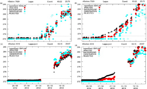
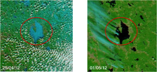
FLake parameterisation in the NHFLAK experiment suggests open water already around 10 April, while MODIS indicates a complete break-up (water clear of ice) around the first day of May (Fig. 6b and d). Analysis of the experiment NHFLAK indicates water clear of ice a few days earlier (24 April) than that of the experiment NHALAK (28 April) (Figs. 6b and a). The visible MODIS-Aqua images (Fig. 7) indicate that Lake Lappajärvi is clear of ice on 1 May but still ice-covered on 25 April. The SYKE observer recorded 2 May as the water clear of ice date for Lake Lappajärvi (see Table 3). SYKE temperature measurements started only on 10 May when the water temperature had already reached 3°C (Figs. 6c and d).

Fig. 7 MODIS-Aqua visible images over Lake Lappajärvi on 25 April (left, 8:30–12:10 UTC) and 1 May (right, 9:50–11:30 UTC), 2012.

The analysis of NHALAK followed MODIS observations more closely than that of NHFLAK, which was influenced by the warmer background suggested by FLake. SYKE temperature measurements were not available before 10 May, entering the NHALAK analysis only well after the observed ice break-up. When there were no MODIS observations over Lake Lappajärvi, the previous analyses that were applied as background in NHALAK would have converged to the climatological values, which still represented ice-covered conditions. If break-up was interpreted from NHALAK analyses based on the observations at the SYKE point alone, it would have occurred 2 weeks later than when MODIS observations were included. In general, melting of Lake Lappajärvi could be described realistically due to the MODIS observations both with and without FLake parameterisations. FLake alone would have led to too early and OI, based only on the (missing) SYKE water temperature measurements and climatology, to too late melting of this lake in the HIRLAM analysis. This is because a lake grid point is assumed to retain its state given by the background field when there are no observations available to correct it.

The reason for the too-early warming of lakes by FLake (noted also in Section 5.2 and in Table 3) requires further study. One possible reason may be related to the missing snow on lake ice. In these experiments, snow parameterisation was included in FLake, as in the reference HIRLAM v. 7.4, but in fact snow never accumulated on lake ice in the model. This was due to a technical error that has lately been corrected.

The rather large variation of MODIS LSWT observations from day to day (Fig. 6), which may result from the unsuccessful removal of the signals due to high-level clouds during preprocessing of the data, poses a problem to the QC within the HIRLAM analysis system. On the other hand, FLake reached (unrealistically) high LSWT after the melt of ice on Lake Lappajärvi. Around 25 May, many MODIS and some SYKE observations were rejected in the background check by the QC, which was not correct in this case. Relations between the adjacent observations of different types (SYKE and MODIS) on the lake and its neighbourhood would require further study. In the present experiments, all lake observations were assumed to have similar statistical properties. For example, the assumed observational error standard deviation was set to 1.5°C for both in-situ and remote-sensing LSWT observations. This value is supported by the evaluation study in paper Part I, where a standard deviation of around 1.8°C was estimated for the satellite measurements for selected 22 Finnish lakes during open-water season when SYKE temperature observations were available.

5.4. Validation of analysis over independent lakes

MODIS UW-L3 LSWT observations were derived but withheld from the HIRLAM analysis over four lakes in Sweden and Russia (see Section 2.3). The Russian Lake Kuito and Lake Valday are chosen for comparison between analyses and observed MODIS LSWT (Fig. 8). These two lakes were chosen for illustration because they are located far enough from the nearest lakes included in the analysis, so that analyses on them are not significantly influenced by the nearby observations. The results for the Swedish Lake Hjälmaren and Lake Bolmen (not shown) confirm the results presented here. The analyses of the three main experiments TRULAK, NHFLAK and NHALAK (Table 2) were compared to MODIS observations during January to May 2012 when results from all experiments were available. MODIS observations with the ice flag −1.2°C (indicating measured temperatures below −0.5°C) were excluded from the set of validation observations. Over these lakes, the analysis by TRULAK and NHFLAK is interpreted directly from the FLake forecast, thus this validation measures the quality of FLake, not that of the analysis method. Similarly, as observations were not applied, validation of NHALAK compares the available climatology to MODIS observations.

Fig. 8 Comparison of LSWT derived by MODIS with LSWT analysed by experiments NHFLAK (SYKE, FLake, MODIS), NHALAK (SYKE, MODIS) and TRULAK (SYKE, FLake) for (a) Lake Valday and (b) Lake Kuito.

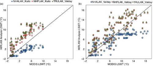
We can see in Fig. 8 that the analyses based on different backgrounds – NHALAK on the previous analysis relaxed towards climatology, TRULAK and NHFLAK on the 6-hour forecast by FLake – started to diverge as soon as the observed LSWT clearly rose above the freezing point. Typically, NHALAK analyses remained significantly colder than MODIS observations, while TRULAK and NHFLAK tended to be significantly warmer. According to the applied climatology, these lakes normally stay ice-covered longer than was observed in spring 2012. Relaxation of the NHALAK towards such a climatology forced the analyses towards freezing temperatures when no observations were available to correct the situation. The warm bias of FLake led the analyses TRULAK and NHFLAK to too high analysed LSWT. This bias was detected earlier in this study as well as by Eerola et al. (2010) and Rontu et al. (2012).

6. Conclusions and outlook

We have reported the first steps in utilising satellite-based observations to define the initial state of lake surfaces in a NWP model. We have applied the HIRLAM surface analysis by introducing new lake observations. While not focussing on optimisation of the analysis methods for LSWT and lake ice, we did however detect their limitations and provided suggestions for improvements. Many questions will require further investigation on the road towards a completely integrated lake data assimilation system for NWP.

In our experiments, we included MODIS and AATSR temperature observations over lakes in HIRLAM. When temperatures below freezing were detected, LSWT was given an ice-flag value, otherwise the observation was assumed to represent the measured LSWT. A limited number of 70 MODIS pixels over 41 large- and medium-size Scandinavian, Karelian and Baltic lakes and a sample of AATSR data over Lake Ladoga were selected for the analysis input. Preprocessing of these data for the analysis is described in paper Part I. To understand the sensitivity of the resulting LSWT analysis to the new data, the analysed LSWT and diagnosed lake ice concentration were compared with those by the experiments where space-borne observations were not included. The initial states of every forecast-analysis cycle of each experiment were validated, mostly qualitatively, against locally recorded freezing and melting dates of the lakes as well as against independent satellite LSWT and ice cover observations. Introduction of space-borne observations led to an improvement of the description of lake surface state, especially during the melt period when in-situ LSWT observations were not yet available and the prognostic lake parameterisations suffered of a significant warm bias. During the freezing period, when the sun was low and weather typically cloudy, only few thermal satellite data were available. In the conditions of well-mixed lake water, typical of the freezing period, the FLake prognostic parameterisations also worked reasonably well, making the additional observations less necessary in autumn.

The background LSWT for the OI analysis was provided either by the prognostic lake parameterisations of the Freshwater Lake model integrated in HIRLAM, or by the previous analysis backed up by climatology. FLake provides background for the LSWT analysis at every HIRLAM grid point containing a lake fraction. In the case of sparse and missing observations, this ensures on average a better result than an analysis that uses the previous analysis as background, especially when the lake is frozen and the background relaxes to climatology. However, in cases where a sufficient quantity of good (satellite-based) observations was regularly available, the analysis using the previously analysed LSWT as the background followed observations closer than when the background LSWT was diagnosed from the predicted FLake lake temperature.

In a case study, MERIS ice fraction over Lake Ladoga was found to qualitatively agree with the ice fraction derived from the HIRLAM lake temperature analysis. Due to the finer spatial resolution of MERIS observations, they provided a more detailed picture than the HIRLAM analysis. However, MERIS is an optical sensor whose data coverage is limited by the presence of clouds. Ice cover observations derived from passive microwave sensors do not suffer from this problem. However, they are presently of a coarse spatial resolution (ca 10 km) and would thus only represent large lakes. The Interactive Multisensor Snow and Ice Mapping System (IMS) product (4 km resolution) could be the other alternative, which utilises a variety of multi-sourced datasets such as passive microwave, visible imagery, operational ice charts and other ancillary data (Helfrich et al., 2007; Ramsay, 1998). IMS data has been shown to be an effective product for lake ice (Brown and Duguay, 2012; Duguay et al., 2011, 2012, 2013; Kang et al., 2012) and sea ice (Brown et al., 2014) phenology studies.

In the long term, for a direct assimilation of ice concentration from optical sensors, some spatialisation methods such as OI should be used. However, solutions for several theoretical and technical problems need to be found. The error distribution of the ice concentration is probably non-Gaussian and needs application of specific methods (Lisaeter et al., 2003; Qin et al., 2009; Simon and Bertino, 2009). For the background, the FLake ice fraction can at the moment only be 0 or 1. This means that it is only known if the lakes in the grid box are ice-covered or not. Such information is in principle qualitative, when defined within the relatively coarse resolution of the NWP model. Methods to assimilate qualitative information are poorly developed in NWP. For example, an algorithm for assimilation of remotely sensed snow extent (Drusch et al., 2004) uses a quite simple and ad-hoc approach. When utilising LSWT and ice cover observations together, it will be necessary to ensure their consistency in the resulting analysis. Experience from simplified methods, where the observed ice fraction is converted to temperature, which is then treated by the OI algorithm together with SST (Canadian Meteorological Centre), may also be helpful. In addition to the horizontal spatialisation, methods to assimilate ice information with respect to the prognostic variables of FLake (such as ice thickness) should be developed.

Extended application of remote-sensing LSWT measurements is a novel feature in this paper, compared to our previous studies (Eerola et al., 2010; Rontu et al., 2012). However, significantly more data, potentially available from satellites, still remain unused with the approach of predefined pixels over the lakes (70 pixels used in this study versus several tens of thousands pixels covered by the satellite measurements). By using the fine-resolution land-cover information available in the NWP model, it is possible to classify if a satellite pixel (with known coordinates) is located over a lake resolved by the model. Thus, it would be possible to utilise high-resolution near-real time satellite LSWT/ice cover observations without pre-selection of pixels. Methods to reduce the amount of input data over large lakes (thinning, screening, creation of super-observations) should be developed and applied in order to avoid giving too much weight to the large amount of mutually correlated satellite data compared to possible in-situ measurements, and also in order to keep the amount of input data reasonable compared to the resolution of the NWP model. Certain preprocessing of these data, including cloud clearance, identification of missing data and estimation of the measurement error in each pixel would be preferable before entering the OI QC within the model.

Improvement of the operational analysis of remote-sensing LSWT measurements in NWP models requires development of the OI methods. Derivation of the autocorrelation functions (structure functions), which take into account lake depth and elevation, as well as calculation of observation error statistics of different measurement types is believed to be important. Practical questions should be resolved in the future, such as: how to obtain near-real-time daily observational data of reasonable volume in a universal format; how to introduce more than selected pixel observations into the analysis; how to improve the QC before and within the NWP application. For the operational NWP models, the analysis of the transient surface properties is crucial, but handing of the observational data and computations should be highly optimised in order to allow timely production of the full three-dimensional weather forecast. Input information should be processed without manual intervention, but well enough to allow only reliable observations to influence the analysis.

It is worth mentioning that presently, the analysed state of the lake surface creates no feedback to the FLake parameterisation, which is coupled to the atmospheric model during the forecast run. Thus, the improved LSWT analysis remains as a possibly useful independent by-product of the NWP model. In order to really utilise the space-borne and in-situ observations on lake surface state for the improvement of the weather forecast and prediction of lake temperatures, methods to connect the analysed LSWT and ice cover to the prognostic in-lake variables are needed. Such methods for NWP models are currently under development (Ekaterina Kurzeneva, personal communication, 2014).

To conclude, it has been learned that space-borne LSWT observations are beneficial for the description of lake surface state in HIRLAM. Satellite observations provide frequent observations over large areas. The large spatial coverage of satellite-based data at a high resolution is a major advantage but also an application challenge when compared to in-situ measurements.

7. Acknowledgements

Our thanks are due to two anonymous reviewers, whose comprehensive comments significantly helped to improve the manuscript. This research was supported by European Space Agency (ESA-ESRIN) Contract No. 4000101296/10/I-LG (Support to Science Element, North Hydrology Project) and a Discovery Grant from the Natural Sciences and Engineering Research Council of Canada (NSERC) to C. Duguay, as well as a NSERC postgraduate scholarship to H. Kheyrollah Pour. The support of the international HIRLAM-B programme is acknowledged. The MERIS lake fraction data was generated and supplied by R. Solberg (Norwegian Computing Center).

References

- Brown L. C. , Duguay C. R . The response and role of ice cover in lake-climate interactions. Prog. Phys. Geogr. 2010; 34(5): 671–704. DOI: 10.1177/0309133310375653.
- Brown L. C. , Duguay C. R . Modelling lake ice phenology with an examination of satellite-detected subgrid cell variability. Adv. Meteorol. 2012; 19: 529064. DOI: 10.1155/2012/529064.
- Brown L. C. , Howell S. E. L. , Morth J. , Derksen C . Evaluation of the Interactive Multisensor Snow and Ice Mapping System (IMS) for monitoring sea ice phenology. Rem. Sens. Environ. 2014; 147: 65–78.
- Daley R . Atmospheric Data Analysis. 1991; New York, NY, USA: Cambridge University Press. 457.
- Donlon C. J. , Martin M. , Stark J. , Robert-Jones J. , Fiedler E. , co-authors . The operational sea surface temperature and sea ice analysis (OSTIA) system. Rem. Sens. Environ. 2012; 116: 140–158.
- Drusch M. , Vasilievic D. , Viterbo P . ECMWF's global snow analysis: assessment and revision based on satellite observation. J. Appl. Meterol. 2004; 43: 1282–1294.
- Duguay C. R. , Brown L. , Kang K.-K. , Kheyrollah Pour H . Lake ice [in Arctic report card 2011]. 2011. Online at: http://www.arctic.noaa.gov/report11/lake_ice .
- Duguay C. R. , Brown L. , Kang K.-K. , Kheyrollah Pour H . [The Arctic] lake ice [in State of the climate in 2011]. Bull. Am. Meteorol. Soc. 2012; 93(7): 152–154.
- Duguay C. R. , Brown L. , Kang K.-K. , Kheyrollah Pour H . [The Arctic] lake ice [in State of the climate in 2012]. Bull. Am. Meteorol. Soc. 2013; 94(8): 124–126.
- Duguay C. R. , Prowse T. D. , Bonsal B. R. , Brown R. D. , Lacroix M. P. , co-authors . Recent trends in Canadian lake ice cover. Hydrol. Proc. 2006; 20: 781–801.
- Eerola K . Twenty-one years of verification from the HIRLAM NWP system. Weather Forecast. 2013; 28: 270–285.
- Eerola K. , Rontu L. , Kourzeneva E. , Shcherbak E . A study on effects of lake temperature and ice cover in HIRLAM. Boreal Environ. Res. 2010; 15: 130–142.
- Fiedler E. , Martin M. , Roberts-Jones J . An operational analysis of lake surface water temperature. Tellus A. 2014; 66: 21247. DOI: 10.3402/tellusa.v66.21247.
- Gandin L . Objective Analysis of Meteorological Fields. 1965; Gidrometizdat, Leningrad. Translated from Russian, Jerusalem, Israel Program for Scientific Translations. 242.
- Grönvall H. , Seinä A . Satellite data use in Finnish winter navigation. Operational Oceanography: Implementation at the European and Regional Scales – Proceedings of the Second International Conference on EuroGOOS. 2002; Elsevier. 429–436. 11–13 March 1999, Rome, Italy, (eds. N. C. Flemming et al.).
- Helfrich S. R. , McNamara D. , Ramsay B. H. , Baldwin T. , Kasheta T . Enhancements to, and forthcoming developments in the Interactive Multisensor Snow and Ice Mapping System (IMS). Hydrol. Process. 2007; 21: 1576–1586.
- Hook S. , Wilson R. C. , MacCallum S. , Merchant C. J . Lake surface temperature. Bull. Am. Meteorol. Soc. 2012; 93: 18–19.
- Kang K.-K. , Duguay C. R. , Howell S. E. L . Estimating ice phenology on large northern lakes from AMSR-E: algorithm development and application to Great Bear Lake and Great Slave Lake, Canada. Cryosphere. 2012; 6(2): 235–254.
- Kheyrollah Pour H. , Duguay C. R. , Martynov A. , Brown L. C . Simulation of surface temperature and ice cover of large northern lakes with 1-D models: a comparison with MODIS satellite data and in situ measurements. Tellus A. 2012; 64: 17614. DOI: 10.3402/tellusa.v64i0.17614.
- Kheyrollah Pour H. , Duguay C. R. , Solberg R. L. C . Impact of satellite-based lake surface observations on the initial state of HIRLAM. Part I: Evaluation of remotely-sensed lake surface water temperature observations. Tellus A. 2014; 66: 21534. DOI: 10.3402/tellusa.v66i0.21534.
- Kourzeneva E. , Asensio H. , Martin E. , Faroux S . Global gridded dataset of lake coverage and lake depth for use in numerical weather prediction and climate modelling. Tellus A. 2012a; 64: 15640. DOI: 10.3402/tellusa.v64i0.15640.
- Kourzeneva E. , Martin E. , Batrak Y. , Le Moigne P . Climate data for parameterization of lakes in NWP models. Tellus A. 2012b; 64: 17226. DOI: 10.3402/tellusa.v64i0.17226.
- Krinner G. , Boike J . A study of the large-scale climatic effects of a possible disappearance of high-latitude inland water surfaces during the 21st century. Boreal Environ. Res. 2010; 15: 203–217.
- Lisaeter K. A. , Rosanova J. , Evensen G . Assimilation of ice concentration in a coupled ice-ocean model, using the Ensemble Kalman Filter. Ocean Dynam. 2003; 53: 358–388. DOI: 10.1007/s10236-003-0049-4.
- Loveland T. R. , Reed B. C. , Brown J. F. , Ohlen D. O. , Zhu J. , co-authors . Development of a global land cover characteristics database and IGBP DISCover from 1-km AVHRR data. Int. J. Remote Sens. 2000; 21: 1303–1330.
- MacCallum S. N. , Merchant C. J . Surface water temperature observations of large lakes by optimal estimation. Can. J. Remote Sens. 2012; 38(1): 25–45. DOI: 10.5589/m12-010.
- Manrique-Suñén A. , Nordbo A. , Balsamo G. , Beljaars A. , Mammarella I . Representing land surface heterogeneity: offline analysis of the tiling method. J. Hydrometeor. 2013; 14: 850–867. DOI: 10.1175/JHM-D-12-0108.1.
- Mironov D . Parameterization of Lakes in Numerical Weather Prediction. Description of a Lake Model.
- Mironov D. , Heise E. , Kourzeneva E. , Ritter B. , Schneider N. , co-authors . Implementation of the lake parametrisation scheme FLake into the numerical weather prediction model COSMO. Boreal Environ. Res. 2010; 15: 218–230.
- Ngai K. L. C. , Shuter B. J. , Jackson D. A. , Chandra S . Projecting impacts of climate change on surface water temperatures of a large subalpine lake: Lake Tahoe, USA. Clim. Change. 2013; 118: 841–855.
- Niziol T. A . Operational forecasting of lake effect snowfall in Western and Central New York. Weather Forecast. 1987; 2: 310–321. DOI: 10.1175/1520-0434(1987)002¡0310:OFOLES¿2.0.CO;2.
- Niziol T. A. , Snyder W. R. , Waldstreicher J. S . Winter weather forecasting throughout the Eastern United States. Part IV: Lake effect snow. Weather Forecast. 1995; 10: 61–77.
- Qin J. , Liang S. , Yang K. , Kaihotsu I. , Liu R. , Koike T . Simultaneous estimation of both soil moisture and model parameters using particle filtering method through the assimilation of microwave signal. J. Geophys. Res. 2009; 114: 15103. DOI: 10.1029/2008JD011358.
- Ramsay B. H . The interactive multisensor snow and ice mapping system. Hydrological Processes. Hydrol. Process. 1998; 12: 1537–1546.
- Rontu L. , Eerola K. , Kourzeneva E. , Vehviläinen B . Data assimilation and parametrisation of lakes in HIRLAM. Tellus A. 2012; 64: 17611. DOI: 10.3402/tellusa.v64i0.17611.
- Samuelsson P. , Kourzeneva E. , Mironov D . The impact of lakes on the European climate as simulated by a regional climate model. Boreal Environ. Res. 2010; 15: 113–129.
- Semmler T. , Cheng B. , Yang Y. , Rontu L . Snow and ice on Bear Lake (Alaska)- sensitivity experiments with two lake ice models. Tellus A. 2012; 64: 17339. DOI: 10.3402/tellusa.v64i0.17339.
- Simon E. , Bertino L . Application of the Gaussian anamorphosis to assimilation in a 3-D coupled physical-ecosystem model of the North Atlantic with the EnEKF: a twin experiment. Ocean Sci. 2009; 5: 495–510.
- Undén P. , Rontu L. , Järvinen H. , Lynch P. , Calvo J . The HIRLAM-5 scientific documentation. 2002. Available at HIRLAM-5 Project, c/o Per Undén SMHI, S-601 76 Norrköping, Sweden. Online at: http://hirlam.org .
- Yang Y. , Cheng B. , Kourzeneva E. , Semmler T. , Rontu L. , co-authors . Modelling experiments on air-snow-ice interactions over Kilpisjärvi, a lake in northern Finland. Boreal Environ. Res. 2013; 18(5): 341–358.
- Zhao L. , Jin J. , Wang S.-Y. , Ek M. B . Integration of remote-sensing data with WRF to improve lake-effect precipitation simulations over the Great Lakes region. J. Geophys. Res. 2012; 117: 09102. DOI: 10.1029/2011JD016979.