Hybrid algorithm of ensemble transform and importance sampling for assimilation of non-Gaussian observations

Abstract

A hybrid algorithm that combines the ensemble transform Kalman filter (ETKF) and the importance sampling approach is proposed. Since the ETKF assumes a linear Gaussian observation model, the estimate obtained by the ETKF can be biased in cases with nonlinear or non-Gaussian observations. The particle filter (PF) is based on the importance sampling technique, and is applicable to problems with nonlinear or non-Gaussian observations. However, the PF usually requires an unrealistically large sample size in order to achieve a good estimation, and thus it is computationally prohibitive. In the proposed hybrid algorithm, we obtain a proposal distribution similar to the posterior distribution by using the ETKF. A large number of samples are then drawn from the proposal distribution, and these samples are weighted to approximate the posterior distribution according to the importance sampling principle. Since the importance sampling provides an estimate of the probability density function (PDF) without assuming linearity or Gaussianity, we can resolve the bias due to the nonlinear or non-Gaussian observations. Finally, in the next forecast step, we reduce the sample size to achieve computational efficiency based on the Gaussian assumption, while we use a relatively large number of samples in the importance sampling in order to consider the non-Gaussian features of the posterior PDF. The use of the ETKF is also beneficial in terms of the computational simplicity of generating a number of random samples from the proposal distribution and in weighting each of the samples. The proposed algorithm is not necessarily effective in case that the ensemble is located distant from the true state. However, monitoring the effective sample size and tuning the factor for covariance inflation could resolve this problem. In this paper, the proposed hybrid algorithm is introduced and its performance is evaluated through experiments with non-Gaussian observations.

• data assimilation
• ensemble filters
• ensemble transform Kalman filter
• Monte Carlo method
• particle filter

1. Introduction

The ensemble-based approach is now recognised as a valuable tool for data assimilation in nonlinear systems. In particular, the ensemble Kalman filter (EnKF) (Evensen, 1994, 2003) and the ensemble square root filters (Tippett et al., 2003; Livings et al., 2008) are widely used in various practical applications. However, since these algorithms basically assume a linear Gaussian observation model like the Kalman filter (KF), they could give biased or incorrect estimates when the observation is nonlinear or non-Gaussian.

The particle filter (PF) (Gordon et al., 1993; Kitagawa, 1996; van Leeuwen, 2009) is an ensemble-based algorithm that is applicable even in cases with nonlinear or non-Gaussian observations. However, the PF tends to be computationally expensive in comparison with other ensemble-based algorithms. One source of the high computational cost is the degeneracy of the ensemble. In the PF, ensemble members are weighted in the manner of the importance sampling (e.g., Liu, 2001; Candy, 2009) and are then resampled with probabilities equal to the weights. After resampling, many of the ensemble members are replaced by duplicates of some particular members with large weights. Consequently, the diversity of the ensemble is rapidly lost by repeating the resampling process. In order to achieve sufficient diversity, the PF usually requires a huge ensemble size, which results in high computational cost.

Many studies have investigated maintaining the ensemble diversity. One approach is based on kernel density estimation, in which a new ensemble is generated by resampling from a smoothed empirical density function (e.g., Musso et al., 2001). The Gaussian resampling approach (Kotecha and Djurić, 2003; Xiong et al., 2006) and the merging PF (Nakano et al., 2007) have also been devised to maintain the ensemble diversity, although these methods consider only the first and second moments rather than the shape of the probability density function (PDF). Another method by which to maintain the ensemble diversity is to improve the distribution for sampling. If we can draw samples from a distribution similar to a posterior PDF, the weights would be well balanced among the samples which would enable us to improve the computational efficiency. Accordingly, several studies have attempted to improve the distribution for sampling. Pitt and Shephard (1999) proposed the auxiliary particle filter, in which the temporal evolution is calculated for each ensemble member after the ensemble is resampled according to the expected score of the prediction for each ensemble member. Recently, van Leeuwen (2010,2011) proposed another algorithm that refers to the observed data in order to obtain the distribution for sampling. Chorin et al. (2010) and Morzfeld et al. (2012) also took a similar approach. Papadakis et al. (2010) proposed the weighted ensemble Kalman filter (WEnKF), in which the distribution for sampling is obtained by the EnKF, and the samples drawn from the distribution are weighted and resampled. Beyou et al. (2013) took the same approach but they used the ensemble transform Kalman filter (ETKF) (Bishop et al., 2001; Wang et al., 2004), which is one of ensemble square root filters, instead of the EnKF.

However, even if the ensemble diversity is well maintained by improving the distribution for sampling, the ensemble size that we can use is not necessarily sufficient to represent non-Gaussian features of the PDF. In practical applications, the ensemble size is usually limited by the available computational resources because a model run for each ensemble member is costly in the forecast step. Indeed, it is not unusual that the allowed ensemble size is much smaller than the system dimension. If the ensemble size N is smaller than the effective system dimension, the ensemble would form a simplex in (N−1)-dimensional space (Julier, 2003; Wang et al., 2004), which is obviously insufficient to represent the third or higher-order moments. In such a situation, the non-Gaussian features cannot be represented even using the importance sampling. In addition, after weighting the ensemble members, some of the members no longer effectively contribute to the estimation. This means that the probability distribution estimation would be based on a substantially smaller sample size than the original sample size. Therefore, for the case in which the ensemble size is limited, the weighting of the ensemble would not necessarily provide a good approximation of the posterior PDF.

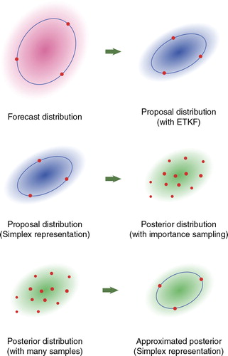
The approach proposed in the present paper considers such a situation in which the forecast PDF is represented by an ensemble of limited size less than the system dimension. Since non-Gaussian features are not represented by the limited-sized ensemble, the proposed approach assumes that the forecast PDF is Gaussian. On the other hand, in the analysis step, we use a sufficiently large number of samples to represent non-Gaussian features of the posterior PDF. These non-Gaussian features are represented by the importance sampling technique (e.g., Liu, 2001; Candy, 2009). An outline of the proposed approach is illustrated in Fig. 1. Before the analysis step, the forecast PDF is represented by an ensemble of limited size that forms a simplex. From this forecast PDF, we obtain a Gaussian proposal PDF, which is similar to but not necessarily identical to the posterior PDF. This proposal PDF is represented by a small ensemble obtained using the ETKF. We then generate a large number of samples from the proposal PDF, and these samples are weighted so as to approximate the posterior PDF. If we use the proposal PDF obtained by the ETKF, we can efficiently generate a large number of samples, which allows us to represent non-Gaussian features of the posterior PDF using the importance sampling technique. For the next forecast step, the approximation of the posterior PDF with a large number of samples is converted into a new approximation with a small ensemble. This small ensemble is constructed under the assumption of a Gaussian distribution, but is obtained after considering the nonlinearity or non-Gaussianity of the observation. We can therefore reduce the effects of the biases due to nonlinear or non-Gaussian observation on the next forecast.

Fig. 1 Outline of the hybrid approach proposed in the present paper.

Various algorithms have been proposed that combine the PF algorithm with a Gaussian-based algorithm, such as the KF and EnKF. For example, several studies considered a Gaussian mixture model and used the KF or EnKF to update each Gaussian component of the Gaussian mixture model (e.g., Smith, 2007; Hoteit et al., 2012). However, a Gaussian mixture model requires a large number of parameters to represent the covariance matrices of each of the Gaussian components for high-dimensional systems and would tend to require too much memory and computational resources. Although Hoteit et al. (2008) proposed another approach that uses a mixture of Gaussian components with the same covariance matrix, their approach assumes a Gaussian observation model. Lei and Bickel (2011) considered another method by which to combine the PF algorithm and the EnKF algorithm, in which the ensemble is adjusted so as to represent the mean and covariance estimated by weighting the members of the forecast ensemble. This approach did not consider an asymmetric probability distribution.

The ETKF algorithms and the importance sampling technique, on which the proposed method is based, are explained in Sections 3 and 4, respectively. Section 5 discusses how to use the ETKF output as a proposal PDF and how to represent the posterior PDF using samples drawn from the proposal PDF. Section 6 discusses how to approximate the posterior PDF with a small-sized ensemble, which allows us to achieve high computational efficiency in the forecast step. We experimentally evaluate the proposed algorithm in Section 8, and provide a summary in Section 9.

2. Sequential data assimilation problem

We describe the state transition of a dynamical system by the following PDF:1

where the vector x _k denotes the state of the system at time t _k (k=1,2,…). We then consider the following observation model to describe the relationship between the system state and the observation:2

where y _k is the observed data at time t _k .

Sequential data assimilation is regarded as a problem that estimates the conditional PDF of the system state x _k from the sequence of observations according to the following recursive procedure. Suppose that the conditional PDF at the time step t _{k − 1}, , is given. Then, the forecast PDF can be obtained by the following equation:3

The observation y _k is then assimilated using Bayes’ theorem to obtain the filtered (analysis) PDF :4

Filtering algorithms for sequential data assimilation estimate the system states based on this filtered PDF. In the following, we discuss how to obtain a good approximation of the filtered PDF.

3. Ensemble transform Kalman filter

In many of the sequential data assimilation algorithms, the exact shapes of the PDFs and are not necessarily considered. In the EnKF, for example, only the mean vector and the covariance matrix are considered. The ETKF, which is classified as an ensemble square-root filter (Tippett et al., 2003; Livings et al., 2008), considers only the mean vector and the covariance matrix.

In the ETKF, the integral of eq. (3) is not computed directly. Instead, the dynamical model is applied to each ensemble member. If the filtered PDF at the previous time t _k−1, is represented by the ensemble , each member of the forecast ensemble can be obtained as follows:5

where is the dynamical model of the system. As described above, the ensemble size N is typically much less than the effective system dimension. In such a situation, the ensemble members form a spherical simplex in a subspace. However, even if the ensemble size N is small, the forecast ensemble obtained by eq. (5) provides good estimates for the mean vector and the covariance matrix of the forecast PDF. As shown by Wang et al. (2004), the mean vector and the covariance matrix of the forecast PDF are estimated considering up to the second-order term of the Taylor expansion of the dynamical model, except that the uncertainties in the complementary subspace are ignored.

The mean vector is represented by the ensemble mean of all of the members:6

The ETKF then considers the deviation from the mean vector as7 8

where the function h _k is a nonlinear predictive observation given a state x _k , and denotes the ensemble mean of the predictive observation as9

The covariance matrix can then be represented as follows:10

Although is sometimes obtained by division by N−1, we obtain by division by N. This is because we assume that the ensemble is not generated by random sampling but that the ensemble is obtained so as to just represent the mean vector and the covariance matrix. Now we define the following matrices11 12

Using the matrix , the ensemble covariance matrix can be written as13

This means that is a square root of the covariance matrix . If we define the dimension of the state vector x _k as M, the matrix is an M×N matrix, and is an M×M matrix. Typically, M is much larger than N. Since the ensemble mean has been subtracted in eq. (7), the rank of the matrix would become N−1, not N. Strictly speaking, the rank of can be less than N−1. However, in practical applications, where M is much larger than N, it would be improbable that the rank of happens to become less than N−1. Therefore, we hereinafter assume that the rank of is N−1.

The ETKF provides an estimate of the mean vector of the posterior PDF as14

and a square root of the covariance matrix of as15

where we indicate the estimate obtained using the ETKF by the dagger †. The matrix in eq. (14) is the Kalman gain used in the conventional KF. The transform matrix is defined such that the matrix satisfies16

In order to obtain the matrices and , the ETKF calculates the eigenvalue decomposition of the matrix . The matrix is the covariance matrix of the observation noise, which is given if the observation model in eq. (2) is assumed to be Gaussian, as17

If the eigenvalue decomposition of is obtained as18

then the matrices and become:19 20

The matrix Φ _k is chosen such that offers an unbiased ensemble satisfying the following condition:21

where and . This condition can be satisfied if Φ _k is set as22

but another choice is allowed as long as it satisfies eq. (21) (Wang et al., 2004; Livings et al., 2008; Sakov and Oke, 2008).

4. Importance sampling

Since the ETKF considers only the mean vector and the covariance matrix, the ETKF implicitly assumes that the forecast PDF is Gaussian (e.g., Lawson and Hansen, 2004). Moreover, if the ensemble size is smaller than the system dimension, it is practically impossible to consider the non-Gaussian features of the forecast PDF. Accordingly, the proposed algorithm assumes (or approximates) that the forecast distribution is Gaussian. The ETKF then provides an estimate of the mean vector and the covariance matrix of the filtered PDF based on KF framework. Since the KF assumes a linear Gaussian observation, the ETKF works well in the case of a linear Gaussian observation. However, if the observation is nonlinear or non-Gaussian, the observation must be approximated by a linear Gaussian model in order to apply the ETKF. In general, the Gaussian approximation of the nonlinear or non-Gaussian observation is not easy. Even if a good approximation could be obtained, approximation errors are inevitably introduced, which might cause a biased estimate or misevaluation of the scale of uncertainty. In order to resolve these problems, we use the importance sampling approach.

The importance sampling (e.g., Liu, 2001; Candy, 2009) is a Monte Carlo approach that approximates a target PDF using a large number of samples from another distribution from which samples can be easily drawn. Using the importance sampling, the filtered PDF can be approximated as follows

where indicates a sample drawn from , and Z is a normalisation factor. The PDF represented by is called the proposal distribution, which can be chosen arbitrarily. If we choose the forecast distribution as the proposal distribution, we obtain the original form of the PF (Gordon et al., 1993; Kitagawa, 1996).

Equation (23) indicates that the filtered PDF can be approximated by weighting the particles drawn from the proposal distribution, where the weight for each particle satisfies:24

The efficiency of the importance sampling depends on the imbalance of the importance weights . If the imbalance of the importance weights among the proposal samples is large, most of the samples are ineffective, and the approximation of the PDF will be poor. According to eq. (23), the imbalance of the weights among the ensemble members can be reduced by choosing a proposal distribution that is similar to the filtered PDF . If we use samples from such a proposal distribution, we can efficiently obtain a good approximation of the posterior PDF. In order to obtain a good proposal distribution, we use the ETKF.

5. Importance sampling with an ETKF-based proposal

For the importance sampling, the estimate of the posterior distribution obtained by the ETKF is used as the proposal distribution. We thus assume that the proposal distribution is a Gaussian distribution with mean and covariance , . Since the actual posterior distribution is not necessarily Gaussian, there can be a discrepancy between the proposal distribution and the posterior distribution. By weighting the proposal ensemble members according to the importance sampling principle, we can resolve this discrepancy and obtain a good approximation of a non-Gaussian posterior distribution. In order to obtain the proposal distribution using the ETKF, we have to use a Gaussian observation model as in eq. (17) even if the observation is non-Gaussian. In such cases, the covariance matrix is not necessarily specified. In obtaining the proposal distribution, the covariance matrix can be chosen arbitrarily. However, it is preferable to choose so as to provide a proposal PDF similar to the posterior PDF in order to achieve the high efficiency.

Using the matrix , which is a square root of as seen in eq. (16), we can draw a sample from according to the following equation:25

where is a random sample drawn from a Gaussian distribution with a zero mean vector and identity covariance matrix26

The dimension of is equal to the number of ensemble members N. In typical data assimilation problems, N is much less than the dimension of the state vector x _k . We can thus easily generate a large number of samples from using eqs. (25) and (26). The generative model described by eqs. (25) and (26) was also considered by Hunt et al. (2007), and is similar to a model of probabilistic principal component analysis (Roweis and Ghahramani, 1999; Tipping and Bishop, 1999; Bishop, 2006). Using this model, the uncertainty of the vector x _k in a very high-dimensional space can be represented by the uncertainty of a latent variable z _k in a low-dimensional space. Accordingly, the proposal distribution is defined in the low-dimensional subspace (Rao, 1973).

In order to approximate the posterior PDF using the samples , it is necessary to calculate and in eq. (23). Considering that is generated from according to eq. (25), is associated with the Gaussian in eq. (26) that generates . However, it should be noted that the rank of the matrix is not N but N−1, because is designed so as to preserve the ensemble mean, as indicated in eq. (21). Although is proportional to , the component associated with 1 can be discarded in . Therefore, as explained in the Appendix, we obtain the following relationship:27

The calculation of requires a few more steps. Using Bayes’ theorem in eq. (4), we have28

The first factor on the right-hand side can be obtained from the observation model in eq. (2). The second factor is obtained from the forecast distribution , which is specified by the mean vector in eq. (6) and the covariance matrix in eq. (13). Assuming that the PDF is Gaussian, we regard as a sample generated from according to the following process:29

where ζ _k is a random vector that obeys the Gaussian distribution with a zero mean vector and an identity covariance matrix. Similarly to eq. (27), we can deduce30

Using eqs. (14), (15) and (19), eq. (25) is reduced to

Comparing eqs. (29) and (31), we can determine the value of as

Despite its complicated form, the calculation of eq. (32) is not expensive because the matrix has already been obtained in the calculation of the Kalman gain in eq. (19). Consequently, the ratio between and in eq. (23) is obtained for each i as

Using eq. (33), we can approximate by the samples drawn from in the following form:34

where J denotes the number of samples drawn from , and the weight is defined as35

Note that J may not be equal to the ensemble size N. Although the ensemble size N would, in practice, be constrained by computational resources in the forecast step, the number of samples from , J, could be taken to be much larger than N. Using a large number of samples from , we can represent the non-Gaussian features of that are due to nonlinearity or non-Gaussianity in the observation.

If the proposal distribution agrees with the filtered distribution , the weights in eq. (35) take the same value for all of the ensemble members. In contrast, if the discrepancy between and is large, the imbalance of the weights becomes large. The discrepancy between and arises from the Gaussian approximation for the non-Gaussian observation model. Thus, the imbalance of the weights would indicate the quality of the Gaussian approximation for the observation model. The imbalance of the weights can be evaluated using a metric called the effective sample size (Liu and Chen, 1995; Liu, 2001), which is defined as36

Otherwise, the imbalance can be evaluated using the entropy (e.g., Pham, 2001):37

Actually, a rough evaluation can be performed using the N ensemble members obtained by the ETKF as they are. The ensemble members obtained by the ETKF can be written in the form of eq. (25) where is given as follows:

Since for all i, the denominator of eq. (33) takes the same value for all i. Thus, it is sufficient to evaluate the numerator of eq. (33) for each ensemble member obtained by the ETKF. The effective sample size J _eff is also useful for determining J. If the effective sample J _eff is small, only a small number of particles contribute to the estimates, which would result in poor accuracy. Thus, J should be determined so as to maintain J _eff to be sufficiently large. This will also be discussed in Section 8.

6. Ensemble reconstruction

Although the weighted ensemble in eq. (34) would provide a good approximation of the posterior distribution, the large ensemble size requires a huge computational cost in the forecast step. In order to achieve high computational efficiency in the forecast step, we must re-approximate the posterior PDF with a small ensemble before the forecast step. According to the PF algorithm, the new ensemble can be generated by resampling such that each ensemble member is drawn with a probability that is proportional to the weight . We could also obtain samples with no duplicates by using rejection sampling (e.g., Liu, 2001), in which a sample drawn from is accepted with a probability that is proportional to and is rejected otherwise.

These methods provide N random samples from . However, the limited number of random samples would introduce serious sampling errors even if is well represented by eq. (34) with a large number of samples. The ETKF, which preserves the mean and covariance of a posterior PDF obtained from an ensemble-based prior, is intrinsically designed so as to exclude such randomness. We consider a strategy by which to obtain N samples that well represent the mean vector and the covariance matrix of . Although such samples could also be obtained by the second-order-exact sampling proposed by Pham (2001), we adopt the following ensemble transform method in order to obtain such samples.

If is represented by eq. (34), the mean vector of is obtained as follows:

where we used40

which can readily be derived from eq. (35). If we write the mean of as41

eq. (39) becomes42

The covariance matrix is obtained as follows:

We write the covariance matrix of as44

and then we have45

The new must satisfy the following conditions (Wang et al., 2004; Livings et al., 2008):46 47

We can obtain such a matrix that satisfies these two conditions as follows. First, considering that as indicated in eq. (21), we discard the component associated with the vector 1. We define the following symmetric matrix48

which is very similar to a matrix introduced by Pham (2001). Since obviously , eq. (45) can be modified as follows:

We then calculate the following eigenvalue decomposition of the matrix :50

The matrix contains an eigenvector that is parallel to 1 and corresponds to the zero eigenvalue because the matrix obviously satisfies51

according to eq. (48). Therefore, if we define as52

then satisfies eqs. (46) and (47). Decomposing the matrix , we obtain the ensemble perturbations:53

Finally, we obtain each member of the filtered ensemble as follows:54

7. Summary of the proposed algorithm

The proposed hybrid algorithm is summarised as follows. We assume that the filtered PDF at time , , is approximated by the following ensemble: . The ensemble representing the filtered PDF at the next time t _k can be obtained as follows:

1. Forecast step.

2. Generation of the proposal distribution using the ETKF.

3. Sampling.

4. Weighting of the proposal particles.

5. Reconstruction of the Gaussian ensemble.

8. Numerical experiments

In this section, we test the proposed hybrid algorithm using the Lorenz 96 model (Lorenz and Emanuel, 1998), which is described by the following equations:55

for , where , , and . We take the dimension of the state vector M to be 40 and the forcing term f to be 8. The time step for integrating the system equation was set to be 0.01. In the following, we compare the hybrid algorithm and the standard ETKF algorithm using three different observation models: a linear Gaussian observation model, a nonlinear Gaussian observation model, and a non-Gaussian observation model.

8.1. Experiment with a linear Gaussian observation

First, we consider the case with the following linear Gaussian observation model:56

where the matrix extracts the observable components from the state vector x _k . The state dimension M was set at 40. We assume that we can observe x _m if m is an even number ; that is, half of the state variables are observed. The matrix is therefore defined such that . In applying the ETKF, we define the observation function h _k for eq. (8) as . We consider two cases with different standard deviations σ, 0.5 and 1.0, for the observation noise. Observations are obtained from the system every 5 time steps.

We compared the hybrid algorithm proposed in the present paper to the standard ETKF algorithm by estimating the system states from the above observation with each algorithm. In assimilating the observations, we performed covariance inflation (Anderson and Anderson, 1999) with an inflation factor of 1.1. We calculated the root-mean-square of the deviation of the estimate from the true state for 50,000 time steps, averaged over all 40 components. The estimate with each algorithm was obtained by the ensemble mean. In order to avoid the dependence of the initial condition, we perform the state estimation for 10,000 time steps before performing the root-mean-square error calculation for 50,000 time steps. In addition, we performed 50 trials with different initial ensembles and the root-mean-square of the deviation from the true state was averaged over the 50 trials. We performed the estimation for various ensemble sizes, N, in the forecast step. For the importance sampling in the hybrid algorithm, the number of Monte Carlo samples J was set to be 16N, that is, 16 times the ensemble size. Table 1 shows the results of the experiments. For both the standard ETKF and the hybrid algorithm, the state estimation sometimes failed to trace the true state if the ensemble size N was taken to be less than a certain threshold. However, if N was larger than the threshold, the accuracy of the estimation did not change significantly or got slightly worse with the increase of N.

Table 1. Results of experiments with the linear Gaussian observation model

RMSE (σ=0.5)		RMSE (σ=1.0)
Hybrid filter	ETKF	Hybrid filter	ETKF
N=16	0.84	0.62	4.31	3.44
N=18	0.18	0.19	0.71	0.50
N=20	0.18	0.19	0.39	0.41
N=24	0.19	0.20	0.39	0.41
N=28	0.19	0.20	0.40	0.42
N=32	0.19	0.20	0.40	0.43
N=36	0.19	0.21	0.40	0.43

When the standard deviation of the observation noise was 0.5, 18 particles were sufficient for estimation using either the proposed hybrid filter or the standard ETKF. When the ensemble size N was taken to be sufficiently large, the root-mean-square of the deviation from the true state was approximately 0.19 with the hybrid filter but was approximately 0.20 with the standard ETKF. When the standard deviation of the observation noise was increased to 1.0, 20 ensemble members were required for both of the filters. When the ensemble size N was sufficiently large, the root-mean-square was 0.39 for the proposed hybrid algorithm and 0.41 for the standard ETKF. Thus, the proposed algorithm provides similar results to the ETKF algorithm for the case with a linear Gaussian observation model. The number of particles required for successful estimation was also the same for both algorithms. Thus, the weighting in eq. (33) provides appropriate results without overfitting. The small difference in the results between the hybrid algorithm and the standard ETKF was possibly due to the rotation of the ensemble at each time step, which could provide some improvement, as discussed by Sakov and Oke (2008). We also changed the sample size for the importance sampling step. The increase of the sample size did not significantly affect the accuracy, although the decrease of the sample size resulted in the failure of the estimation. If the standard PF (Gordon et al., 1993; Kitagawa, 1996) is used, more than 100 thousands particles are required in order to achieve an accuracy comparable to that of the ETKF and the hybrid algorithm. The proposed hybrid algorithm thus converges with a smaller sample size than the standard PF. In addition, the proposed hybrid algorithm requires far fewer ensemble members for the forecast step.

8.2. Experiment with a nonlinear observation with Gaussian noises

Next, we performed experiments with nonlinear observations with Gaussian noises. We assumed the following observation model:57

where the function h was defined such that . In applying the ETKF, this function h _k is used as the observation function in eq. (8) as it is. Again, the data for the experiments was generated every 5 time steps, and we consider two cases with different standard deviations σ, 0.5 and 1.0, for the observation noise.

In this experiment, the number of Monte Carlo samples used for the importance sampling, J, was adaptively changed at each assimilation step. In the previous experiment with the linear Gaussian observation, the effective sample size was always equal to J and it was maintained by taking J to be sufficiently large. However, when the observation is nonlinear, the effective sample size J _eff can be much smaller than J. Then, if J _eff was less than the threshold, additional Monte Carlo samples were added. In evaluating J _eff, 5N Monte Carlo samples were drawn at once. If J _eff was less than the threshold, additional 5N Monte Carlo samples were drawn in order to increase the number of the Monte Carlo samples. In this way, the Monte Carlo samples were added until the effective sample size exceeded the threshold. Here, the threshold was taken to be 16N. The inflation factor was fixed to be 1.1 again. We then calculated the root-mean-square of the deviation of the estimate from the true state for 50,000 time steps, averaged over all 40 components.

Table 2 shows the root-mean-square of the deviation averaged over 50 trials. When the standard deviation of the observation noise was 0.5, 18 particles were required both for the proposed hybrid filter and for the standard ETKF. The root-mean-square of the deviation from the true state was 0.19 with the hybrid filter and it was 0.20 with the standard ETKF. The results were almost the same as for the linear Gaussian cases, probably because the non-Gaussianity is not significant when the observation noise was taken to be small. When the standard deviation of the observation noise was increased to 1.0, 32 particles were sufficient for the hybrid filter. For the standard ETKF, if N is increased up to 36, the true state was successfully traced for all the 50 trials and the root-mean-square of the deviation was similar for all the 50 trials. Thus, 36 particles would be sufficient for the standard ETKF. The root-mean-square of the deviation was only 0.43 for the proposed algorithm. On the other hand, the root-mean-square of the deviation was 0.59 with the standard ETKF. Thus, when the observation noise was large, the nonlinear observation model would result in high non-Gaussianity and the proposed hybrid algorithm provided better estimates than the standard ETKF. The standard PF required more than 200 thousand particles to achieve an accuracy comparable to that of the hybrid algorithm. The proposed hybrid algorithm converged with a much smaller sample size than the PF.

Table 2. Results of experiments with the nonlinear Gaussian observation model

RMSE (σ=0.5)		RMSE (σ=1.0)
Hybrid filter	ETKF	Hybrid filter	ETKF
N=16	1.36	2.24	5.15	4.93
N=18	0.19	0.20	4.79	4.69
N=20	0.19	0.20	2.96	3.89
N=24	0.19	0.21	1.33	1.12
N=28	0.19	0.21	0.89	0.79
N=32	0.20	0.21	0.43	0.68
N=36	0.20	0.22	0.43	0.59

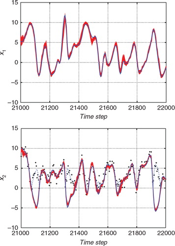
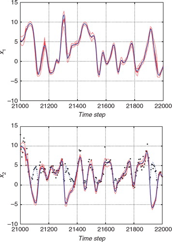
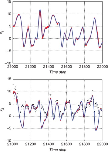
Figures 2 and 3 show the estimates for a certain time interval with the standard ETKF algorithm and the proposed hybrid algorithm, respectively. In each figure, the upper panel shows the estimate for x ₁, which is an unobserved variable, and the lower panel shows the estimate for x ₂, which is an observed variable. The blue lines indicate the true state. The thick red lines indicate the estimates deduced by the ensemble mean and the thin dashed red lines indicate the 2σ range of the filtered (posterior) distribution. The black crosses in the lower panels indicate the observations. Since the function h in eq. (57) includes an operation that takes absolute values, the observations cannot have negative values. For the convenience of the comparison with the observations, the absolute value of the true state is also plotted with the thin blue dashed lines for x ₂. The ensemble size was taken to be 36 for Fig. 2 and 32 for Fig. 3.

Fig. 2 Result of the estimation from the nonlinear observation with the standard ETKF algorithm. The upper panel shows the estimate for x ₁ (an unobserved variable) and the lower panel shows the estimate for x ₂ (an observed variable). The blue line indicates the true state. The red line indicates the estimate. The thin red dashed lines indicate the 2σ range of the filtered distribution.

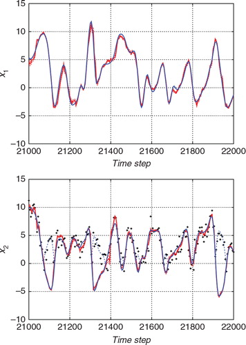
Fig. 3 Result of the estimation from the nonlinear observation with the hybrid algorithm. As in Fig. 2, the upper and lower panels show the estimates for x ₁ (an unobserved variable) and the estimate for x ₂ (an observed variable), respectively. The blue line indicates the true state and the red line indicates the estimate. The thin red dashed lines indicate the 2σ range of the filtered distribution.

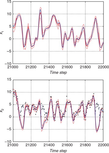
In Fig. 3, the blue line was mostly within the 2σ range of the estimate. On the other hand, in Fig. 2, the true trajectory frequently strayed out of the 2σ range of the ETKF estimate, which indicated that the ETKF sometimes underestimate the uncertainty. The 2σ range for the results obtained using the ETKF tended to be smaller than that for the results obtained using the hybrid filter. Since we cannot distinguish between positive values and negative values in the observation model in eq. (57), the uncertainty should be larger than in the linear observation case. However, the ETKF calculates the state covariance matrix by assuming the linear observation. This would be the reason why the uncertainty estimated using the ETKF was smaller than that estimated using the proposed hybrid algorithm.

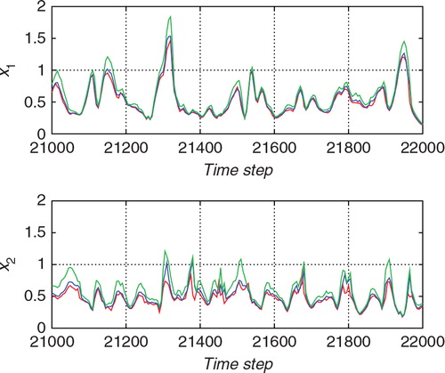
Figure 4 shows the temporal variations of the standard deviations for the forecast (prior) distribution (green line), the proposal distribution (blue line), and the filtered (posterior) distribution (red line), which were obtained by the proposed hybrid filter. The upper and lower panels shows those for x ₁ and x ₂, respectively. Comparing the forecast distribution and the proposal distribution, the uncertainty was largely reduced at most of the observation times. However, the update from the forecast distribution to the proposal distribution was sometimes less effective. In such cases, the update from the proposal distribution to the filtered distribution was more important. The uncertainty was sometimes enlarged at the update from the proposal distribution to the filtered distribution. This would be due to the ambiguity of the observation which cannot discriminate between positive and negative values.

Fig. 4 The standard deviations of the forecast distribution (green line), the proposal distribution (blue line), and the filtered distribution (red line) for the estimation from the nonlinear observation with the hybrid algorithm. The upper and lower panels show the standard deviations for x ₁ (an unobserved variable) and those for x ₂ (an observed variable), respectively.

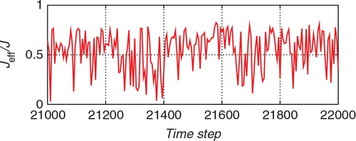
The number of particles used for the importance sampling step, J, is shown in Fig. 5. Although a large number of particles were sometimes used, J was mostly around 1000. A large number of particles were required because the proposal distribution obtained by the ETKF did not provide a good approximation of the posterior distribution. Figure 6 shows the ratio of the effective sample size J _eff to the total size J. This ratio indicates the similarity between the proposal distribution and the posterior distribution. If the proposal distribution is identical to the posterior distribution, the ratio becomes 1. If the discrepancy between the two distributions is large, the ratio becomes small (the minimum is 1/J). Although the ratio was mostly larger than 0.5, it was sometimes small, which means that the ETKF did not provide a good approximation of the posterior distribution.

Fig. 5 The number of particles used for the Monte Carlo step J for the estimation from the nonlinear observation with the hybrid algorithm.

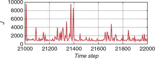
Fig. 6 The ratio between the effective sample size J _eff and J for the estimation from the nonlinear observation with the hybrid algorithm.

The robustness of the estimates was also evaluated by checking the results of the 50 trials. In Figs. 7 and 8, the 50 red lines are plotted and each red line corresponds to the estimate (ensemble mean) for a different trial with a different initial ensemble. The ensemble size was taken to be 36 for Fig. 7 and 32 for Fig. 8, respectively. In both the figures, the 50 estimates follow similar trajectories. Comparing the two figures, however, the results for the ETKF were more dispersed than those for the hybrid algorithm. In this experiment, the proposed hybrid algorithm was more robust than the ETKF.

Fig. 7 Superposition of 50 trials of the estimates from the nonlinear observation with the standard ETKF algorithm (red lines) and the true state (blue line). The upper and lower panels show the estimates for x ₁ (an unobserved variable) and the estimate for x ₂ (an observed variable), respectively.

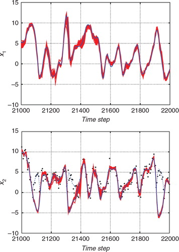
Fig. 8 Superposition of 50 trials of the estimates from the nonlinear observation with the hybrid algorithm (red lines) and the true state (blue line). The upper and lower panels show the estimates for x ₁ (an unobserved variable) and the estimate for x ₂ (an observed variable), respectively.

Table 2 shows that the root-mean-square of the deviation was larger for the proposed algorithm than for the standard ETKF when N was 24 or 28. As mentioned above, when the ensemble size was less than 32, both the proposed algorithm and the standard ETKF sometimes failed to trace the true state. The difference in the value of the root-mean-square of the deviation was likely to be due to the performance after the failure of the estimation. In comparison with the standard ETKF, the proposed filter was likely to be less effectual to recover to the true state again after the true trajectory was missed. Thus, once the estimate failed, the estimate with the proposed filter largely deviated from the truth for a longer time than that with the standard ETKF. That would be the main reason why the error values tended to be larger for the proposed filter than for the standard ETKF when the ensemble size was 24 or 28.

As a matter of fact, when the ensemble largely deviates from the truth, the proposal distribution obtained by the ETKF could be poor in nonlinear or non-Gaussian observation cases. A linear approximation of the observation would be valid if the ensemble is located in the vicinity of the true state and the observations. However, in cases that the ensemble is located distant from the true state, the nonlinearity or non-Gaussianity in the observation could significantly affect the structure of the posterior distribution, and the posterior distribution could be largely distorted from a Gaussian distribution. In such a situation, the Gaussian proposal distribution obtained using the ETKF would have a large difference from the posterior distribution. If the discrepancy between the proposal distribution and the posterior distribution is large, the ratio of the effective sample size to the total sample size would become small. Indeed, during the periods when the ensemble was distant from the truth in the experiments in the present paper, a prohibitively large number of particles were required in order to maintain the effective sample size.

In the experiments shown in the present paper, we restricted the total number of the particles, J _lim, to an upper limit at 1000N in order to reduce the computational cost. When the effective sample size did not reach the threshold J _th even at the upper limit of the total number of the particles, the weights were modified so as to relax the weight imbalance as follows:58

where α is set to be so as to maintain the effective sample size approximately larger than the threshold J _th. However, the accuracy of the approximation of the posterior distribution would be degraded by these treatments. Thus, when the ensemble largely deviate from the truth, the performance of the proposed hybrid algorithm is not necessarily good. This property would also affect the performance at early stage of data assimilation. If the initial state is unknown, the initial ensemble might be located distant from the truth. Therefore, the proposed filter would tend to require more time steps to reach the stable state estimation.

In practice, however, the time steps required to reach stability could be improved by setting the factor for covariance inflation to be larger. Indeed, in this experiment, if the inflation factor was increased to be 1.15, the efficiency of the proposed algorithm for reaching the true state is remarkably improved. In order to evaluate the efficiency to reach the stable estimation, we performed experiments for a situation that the initial state is unknown. An initial ensemble was generated via random sampling from the Gaussian distribution where the mean is 2 and the variance is 2.5 for all of the 40 components, and the time steps required for reaching the stable estimation were examined for each ensemble. Here, we judged that the ensemble reached stability if the root-mean-square of the deviation averaged over all of the 40 components was less than 1.0. When the inflation factor was 1.1, the proposed filter required approximately 3200 time steps on average in order to reach the stable estimation. On the other hand, the ETKF required approximately 940 time steps on average. When the factor for covariance inflation is increased to be 1.15, the proposed filter and the ETKF required approximately 1070 time steps and 970 time steps on average, respectively. Thus, if the inflation factor was taken to be large, the time required for the convergence for the proposed filter became comparable to that for the ETKF.

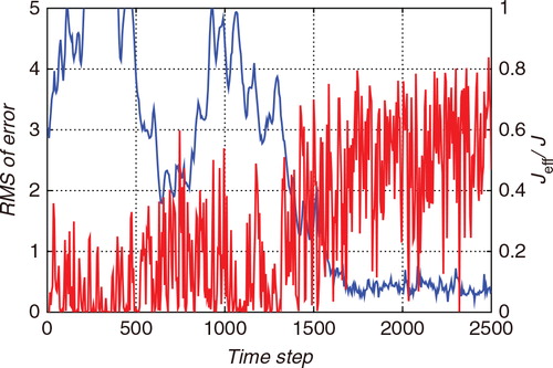
If the increase of the inflation factor significantly improves the performance during periods when the estimate deviates from the true state, it could be practically effective to adaptively change the inflation factor. In practical applications, the true state would be unknown. However, the convergence could be captured by monitoring the effective sample size. Figure 9 compares the ratio of the effective sample size J _eff to the total size J (red line) with the root-mean-square of the deviation from the truth (blue line) in the early stage of data assimilation for one trial in which N=32 and σ=1.0. The variation of the ratio J _eff/J was somewhat noisy. However, when the estimate largely deviated from the truth, the ratio J _eff/J tended to be small. After reaching the stable estimation, the ratio J _eff/J tended to be larger.

Fig. 9 Comparison between the root-mean-square of the deviation from the truth (red) and the ratio of the effective sample size J _eff to the total size J (blue) in the early stage of data assimilation.

8.3. Experiment with a non-Gaussian observation

Finally, we performed experiments with non-Gaussian observations. We assumed the following log-normal observation model:59

Again, the data for the experiments was generated every 5 time steps. We consider two cases with different σ, 0.2 and 0.4 here.

In using the standard ETKF, the observation model in eq. (59) had to be modified because the ETKF assumes linear Gaussian observations. Although the observations were generated by the log-normal model in eq. (59), we used a Gaussian observation model for the estimation with the standard ETKF. In eq. (59), is maximised at for each i(). Accordingly, the Gaussian observation model for the standard ETKF was defined as:60

σ′ was set to be 0.6 for the case that σ=0.2 and 1.2 for the case that σ=0.4. The proposal PDF in the hybrid algorithm was also calculated using this Gaussian observation model. As in the previous experiment, the number of Monte Carlo samples for the importance sampling, J, was adaptively changed at each assimilation step so that the effective sample size was maintained above 16N. The inflation factor was fixed to be 1.1, as in the previous experiments.

We then calculated the root-mean-square of the deviation of the estimate from the true state for 50,000 time steps, averaged over all 40 components and over 50 trials. The results are shown in Table 3. When σ was 0.2, the hybrid filter required 18 particles and the ETKF required 20 particles. The root-mean-square of the deviation from the true state was 0.12 for the hybrid filter while it was 0.20 for the standard ETKF. When σ was 0.4, the hybrid filter required 32 particles. The ETKF sometimes failed even if N was increased to 36. The root-mean-square of the deviation was 0.28 with the proposed algorithm. On the other hand, the root-mean-square was 0.71 with the standard ETKF when N=36, although some failures were included. We performed the experiments with various values of σ′ in eq. (60). However, the standard ETKF did not achieve better results than in the case shown in Table 3. The standard PF required 4 million of particles to attain an accuracy comparable to that of the proposed hybrid algorithm. Thus, the proposed hybrid algorithm exhibited much higher performance than the PF in this experiment again.

Table 3. Results of experiments with the non-Gaussian observation model

RMSE (σ=0.2)		RMSE (σ=0.4)
Hybrid filter	ETKF	Hybrid filter	ETKF
N=16	1.60	2.90	4.90	4.79
N=18	0.12	1.50	4.77	4.63
N=20	0.12	0.20	2.35	3.58
N=24	0.13	0.21	0.91	1.32
N=28	0.13	0.21	0.44	0.89
N=32	0.13	0.21	0.28	0.81
N=36	0.13	0.21	0.28	0.71

Figures 10 and 11 show the estimates for a certain time interval with the standard ETKF algorithm and the hybrid algorithm, respectively. In each figure, the upper panel shows the estimate for x ₁, which is an unobserved variable, and the lower panel shows the estimate for x ₂, which is an observed variable. The blue lines indicate the true state. The thick red lines indicate the estimates deduced by the ensemble mean, and the thin dashed red lines indicate the 2σ uncertainty of the posterior distribution. The black crosses in the lower panels indicate the observations that were transformed as for convenience of comparison with the observations. Since the observations given by eq. (59) cannot distinguish whether x _i is positive or not, each observation is plotted as a positive value. In order to compare the observations with the true state, the absolute value of the true state is also plotted with the thin blue dashed lines for x ₂. The ensemble size was taken to be 36 for Fig. 10 and 32 for Fig. 11, respectively.

Fig. 10 Result of the estimation from the non-Gaussian observation with the standard ETKF algorithm. The upper and lower panels show the estimates for x ₁ (an unobserved variable) and the estimate for x ₂ (an observed variable), respectively. The blue line indicates the true state and the red line indicates the estimate. The thin red dashed lines indicate the 2σ range of the filtered distribution.

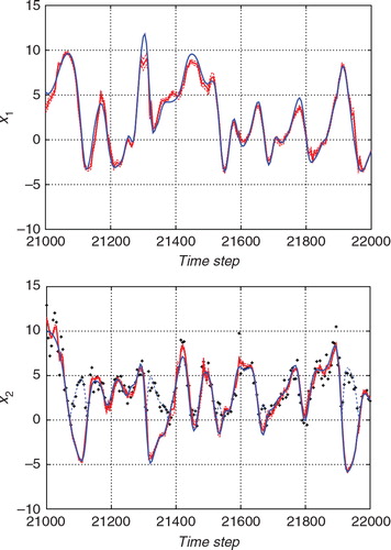
Fig. 11 Result of the estimation from the non-Gaussian observation with the hybrid algorithm. The upper and lower panels show the estimates for x ₁ (an unobserved variable) and the estimate for x ₂ (an observed variable), respectively. The blue line indicates the true state and the red line indicates the estimate. The thin red dashed lines indicate the 2σ range of the filtered distribution.

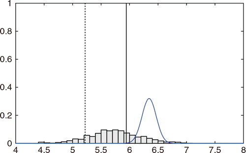
While the ETKF results in Fig. 10 sometimes deviated from the true trajectory, the hybrid algorithm in Fig. 11 successfully estimated the true temporal evolution. In Fig. 10, the 2σ range tended to be smaller than that in Fig. 11. Thus, the ETKF underestimated the uncertainty. If the uncertainty is estimated too small, the observation would not effectively correct the estimate. This would cause larger errors in the ETKF result. For clarity, Fig. 12 compares the two algorithms in terms of the marginal of the filtered distribution of x ₂ at the time step 21,600(t=216.00). The histogram indicates the estimate obtained using the proposed algorithm, and the blue line indicates the marginal distribution estimated using the ETKF. The solid vertical line indicates the true state, and the dashed vertical line indicates the observed value. The proposed algorithm successfully provides a PDF that covers the true state. However, the ETKF effectively misses the true state. The mean of the PDF largely deviates from the true state, and the width of the PDF obtained using the ETKF is too narrow. Since the ETKF assumes a linear Gaussian observation model, the estimate with the ETKF can be biased due to the nonlinear or non-Gaussian observations. In the hybrid algorithm, the importance sampling procedure allows us to effectively resolve such biases.

Fig. 12 Histogram of marginal of the filtered distribution of x ₂ at time step 21600 (t=216.00) for the case with the non-Gaussian observation. The estimate using the ETKF (blue line), the true state (solid vertical line), and the observed value (dashed vertical line) are also shown.

Figure 13 shows the temporal variations of the standard deviations for the forecast (prior) distribution (green line), the proposal distribution (blue line), and the filtered (posterior) distribution (red line), obtained using the proposed hybrid filter. The upper panel shows the estimate for x ₁, and the lower panel shows the estimate for x ₂. In contrast with the previous experiment (see Fig. 4), it seemed that the update from the proposal distribution to the filtered distribution was also effective in this experiment especially for the observed variable x ₂. For example, around the time step 21,200, although the blue line tends to be similar to the red line in the bottom panel of Fig. 4, the blue line tends to be similar to the green line in the bottom panel of Fig. 13. This difference would indicate that a larger improvement was required for the case of a non-Gaussian observation. Figure 14 shows the number of particles used for the importance sampling step, J, and Fig. 15 shows the ratio of the effective sample size J _eff to J. The ratio J _eff/J tended to be lower in Fig. 15 than in Fig. 6. This indicates that the discrepancy between the Gaussian model in eq. (60) and the non-Gaussian model in eq. (59) tended to be large. Since the discrepancy of the proposal distribution from the posterior distribution was large, many of the J particles were ineffective. Figures 16 and 17 show the results for 50 different trials with different initial ensembles. The results for the ETKF were dispersed and sometimes largely deviated from the true trajectory. In contrast, the 50 estimates obtained using the proposed hybrid algorithm followed similar trajectories and provided more robust results than the ETKF.

Fig. 13 The standard deviations of the forecast distribution (green line), the proposal distribution (blue line), and the filtered distribution (red line) for the estimation from the non-Gaussian observation with the hybrid algorithm. The upper and lower panels show the standard deviations for x ₁ (an unobserved variable) and those for x ₂ (an observed variable), respectively.

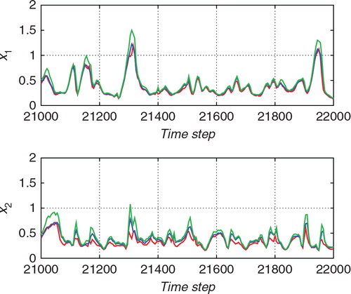
Fig. 14 The number of particles used for the Monte Carlo step J for the estimation from the non-Gaussian observation with the hybrid algorithm.

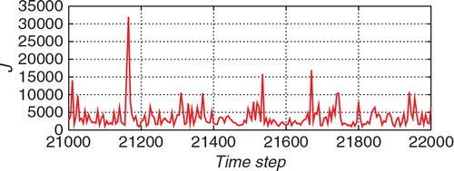
Fig. 15 The ratio between the effective sample size J _eff and J for the estimation from the non-Gaussian observation with the hybrid algorithm.

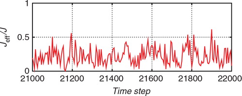
Fig. 16 Superposition of 50 trials of the estimates from the non-Gaussian observation with the standard ETKF algorithm (red lines) and the true state (blue line). The upper and lower panels show the estimates for x ₁ (an unobserved variable) and the estimate for x ₂ (an observed variable), respectively.

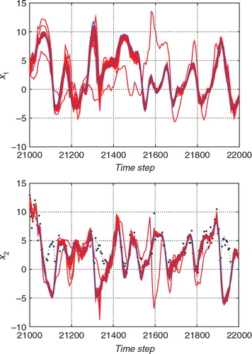
Fig. 17 Superposition of 50 trials of the estimates from the non-Gaussian observation with the hybrid algorithm (red lines) and the true state (blue line). The upper and lower panels show the estimates for x ₁ (an unobserved variable) and the estimate for x ₂ (an observed variable), respectively.

For this experiment with non-Gaussian observation, the proposed filter required approximately 1470 time steps on average in order to reach the stable estimation from the initialisation. On the other hand, the ETKF required approximately 660 time steps on average. If the factor for covariance inflation is increased to be 1.15, the proposed filter and the ETKF required approximately 950 and 930 time steps on average, respectively. As seen in the experiments with nonlinear observation, the proposed filter required a longer time to reach the stable state estimation than the ETKF. However, the increase of the inflation factor remarkably improved the time to reach stability for the proposed filter again.

9. Concluding remarks

We proposed a hybrid algorithm that combines the ETKF and the importance sampling approach. In the proposed algorithm, we first obtain a proposal distribution that is similar to the posterior distribution by using the ETKF. From the proposal distribution obtained using the ETKF, we can efficiently generate a large number of samples. Since this proposal distribution can be biased due to nonlinear or non-Gaussian observations, the samples from the proposal distribution are weighted so as to eliminate the bias by using the importance sampling method. The weight for each sample in the importance sampling can also be calculated very efficiently. Although this weighted ensemble would provide a good approximation of the posterior distribution, its large ensemble size requires a huge computational cost in the forecast step. In order to achieve high computational efficiency in the forecast step, we remake a new ensemble with a small size on the basis of the Gaussian approximation of the posterior PDF.

A similar algorithm has been proposed called the WEnKF (Papadakis et al., 2010), which also combines the Monte Carlo approach and the EnKF. Whereas the proposed hybrid algorithm considers the importance sampling as described in eq. (23), the WEnKF is based on the general PF approach (e.g., Doucet et al., 2000):61

where the weight can be obtained by the following equation62

The WEnKF relies on the Monte Carlo approach which allows non-Gaussianity of the forecast distribution. This is one of the advantages of the WEnKF in contrast with the proposed algorithm which assumes a Gaussian forecast PDF represented with a small-sized ensemble. However, if the PF equation given by eq. (61) is used, the variance of the weights cannot be zero even if the observation is linear and Gaussian (e.g., Ades and van Leeuwen, 2012), which means that the effective sample size is always less than the total sample size. In the proposed algorithm, if the observation is linear and Gaussian, the effective sample size is always equal to the total sample size. The proposed algorithm aims at increasing the efficiency by using the formula which ensures that all the particles can contribute to the estimation in the case with linear Gaussian observation. However, it should be noted that the high efficiency of the proposed algorithm is not guaranteed for the case of nonlinear or non-Gaussian observation. The efficiency of the proposed algorithm would depend on the goodness of obtained by the ETKF.

In eq. (25), the proposal samples are generated in a subspace spanned by the ensemble members for a prior PDF. Accordingly, the posterior PDF is also confined to the same subspace, and the uncertainty in the orthogonal complement space is ignored. On the analogy of the model of the probabilistic principal component analysis (Roweis and Ghahramani, 1999; Tipping and Bishop, 1999; Bishop, 2006), we might be able to consider a small uncertainty in the complement space as follows63

where is a random sample representing the uncertainty of the orthogonal complement space. However, in the case that the dimension of the state vector M is large, an enormous number of samples would be required to appropriately represent the PDF on the high-dimensional space, which would be impossible in practice. The explosion of the number of required samples in high-dimensional problems is referred to as the ‘curse of dimensionality’ (Snyder et al., 2008). To tell the truth, the proposed algorithm breaks the curse of dimensionality by confining the PDF to only a small subspace and ignoring the uncertainty on the complement space. The primary problem caused by the ignorance of the uncertainty of the complement space is that unrealistic, spurious correlations between distant locations are introduced. Such spurious correlations would be resolved by the localisation technique (Ott et al., 2004; Hunt et al., 2007). It could also be effective to add a new member in the complement space according to Song et al. (2010). Therefore, in practical applications, it would not be necessary to use random samples representing the uncertainty of the orthogonal complement space.

In the present study, we assume that the forecast PDF is represented by a limited-sized ensemble. (Wang et al., 2004) discussed the accuracy of the forecast with a limited-sized ensemble, and showed that the forecast ensemble provides the estimates of the mean vector and the covariance matrix of the forecast PDF by considering up to the second-order term of the Taylor expansion of the dynamical model except that the uncertainties in the complementary subspace are ignored. The forecast with a limited-sized ensemble thus considers the nonlinearity in the dynamical model to some extent.

As discussed in the introduction section, the limited-sized ensemble cannot represent the non-Gaussianity of the PDF. This is the reason why we assumed that the forecast ensemble provides a Gaussian approximation of the forecast PDF. In general, however, if the dynamical system is nonlinear, the forecast PDF obtained by eq. (3) is non-Gaussian. Moreover, since the forecast ensemble ignores some parts of the nonlinearity, we cannot obtain the exact mean vector and covariance matrix of the forecast PDF. The representation of the forecast PDF therefore remains as a matter to be studied further.

If the ensemble is located distant from the true state, the nonlinearity or non-Gaussianity of the observation could significantly affect the structure of the posterior distribution. Thus, the Gaussian proposal distribution obtained using the ETKF might not provide a good guess for the posterior distribution. If the discrepancy between the proposal distribution and the posterior distribution is large, the efficiency of the importance sampling would be degraded seriously. For this reason, the proposed algorithm is not necessarily effective when the ensemble largely deviate from the true state. This problem would also deteriorate the performance of the proposed algorithm at early stage of data assimilation. However, the experimental result suggested that this problem might be resolved by tuning the factor for covariance inflation. Even if the true state is unknown, the convergence to stability would be captured by monitoring the effective sample size. Therefore, it could be effective to adaptively change the inflation factor in practice.

11. Appendix

A Probability density for a proposal sample

Importance sampling requires the calculation of the probability that each proposal sample is drawn, which is denoted by in eq. (23). Since the proposal sample is generated by the model of eqs. (25) and (26), the proposal PDF could be associated with the latent variable z _k . However, it should be noted that even if a sample from the proposal PDF is given, the corresponding vector cannot be uniquely specified, because the rank of the matrix is N−1, which is smaller than N, the dimension of z _k . When z _k is converted onto the space of x _k according to eq. (25), one of the components of the vector z _k that is parallel to the vector 1 is projected onto the null space, as indicated in eq. (21). This component is thus redundant for representing . We then discard the component that is associated with 1 in the calculation of for each i.

We consider the following singular-value decomposition of the matrix as

(A1) where the matrix is an M×N matrix consisting of N orthonormal vectors

(A2) Γ is a diagonal matrix

and is an N×N orthogonal matrixA4

One of the column vectors in the matrix will be parallel to 1. Without loss of generality, we can assume that is parallel to 1. Considering that must be satisfied for all i, is given as follows:A5

Since is projected onto the null space, we haveA6

Thus, the N-th components of and will not contribute to . We define matrices that are obtained by truncating the N-th components of and :A7 A8

and a matrix that is obtained by truncating the N-th component of Γ:

eq. (A1) is then reduced toA10

We can rewrite the generative model of eq. (25) asA11

We define a vector asA12

The matrix is orthonormal, and is a sample from the Gaussian distribution with a zero mean vector and an identity covariance matrix. Therefore, the vector can also be regarded as a sample from the Gaussian distribution with a zero mean vector and an identity covariance matrix; that is,A13

If we define a vector that is obtained by truncating the N-th component of :A14

it is regarded as a sample from the Gaussian distribution as:A15

By definition, the vector is associated with asA16

Using this equation, eq. (A11) can be modified asA17

This equation can be rewritten in the following form:A18

which indicates that is uniquely obtained if is given. Therefore, the proposal density at can be associated with the density on the -subspace. Since the relationship between and is linear, is proportional to the probability density of . As obeys a Gaussian distribution in eq. (A15), we obtainA19

Using eqs. (A5), (A12), and (A14), can be calculated as follows:

Therefore,A21

10. Acknowledgements

The present study was supported in part by the Japanese Ministry of Education, Science, Sports and Culture through a Grant-in-Aid for Young Scientists (B), 19740306. The author appreciates many valuable comments provided by the referees.

References

- Ades M. , van Leeuwen P. J . An exploration of the equivalent weights particle filter. Q. J. Roy. Meteorol. Soc. 2012; 139: 820–840.
- Anderson J. L. , Anderson S. L . A Monte Carlo implementation of the nonlinear filtering problem to produce ensemble assimilations and forecasts. Mon. Weather Rev. 1999; 127: 2741.
- Beyou S. , Cuzol A. , Gorthi S. S. , Mémin E . Weighted ensemble transform Kalman filter for image assimilation. Tellus A. 2013; 65: 1–17.
- Bishop C. H. , Etherton R. J. , Majumdar S. J . Adaptive sampling with the ensemble transform Kalman filter. Part I: theoretical aspects. Mon. Weather Rev. 2001; 129: 420–436.
- Bishop C. M . Pattern Recognition and Machine Learning. 2006; Springer, New York.
- Candy J. V . Bayesian Signal Processing–Classical, Modern, and Particle Filtering Methods. 2009; John Wiley, Hoboken..
- Chorin A. J. , Morzfeld M. , Tu X . Implicit particle filters for data assimilation. Commun. Appl. Math. Comput. 2010; 5: 221–240.
- Doucet A. , Godsill S. , Andrieu C . On sequential Monte Carlo sampling methods for Bayesian filtering. Stat. Comput. 2000; 10: 197–208.
- Evensen G . Sequential data assimilation with a nonlinear quasi-geostrophic model using Monte Carlo methods to forecast error statistics. J. Geophys. Res. 1994; 99(C5): 10143.
- Evensen G . The ensemble Kalman filter: theoretical formulation and practical implementation. Ocean Dynam. 2003; 53: 343.
- Gordon N. J. , Salmond D. J. , Smith A. F. M . Novel approach to nonlinear/non-Gaussian Bayesian state estimation. IEE Proceedings F. 1993; 140: 107.
- Hoteit I. , Luo X. , Pham D.-T . Particle Kalman filtering: a nonlinear Bayesian framework for ensemble Kalman filters. Mon. Weather Rev. 2012; 140: 528–542.
- Hoteit I. , Pham D.-T. , Triantafyllou G. , Korres G . A new approximate solution of the optimal nonlinear filter for data assimilation in meteorology and oceanography. Mon. Weather Rev. 2008; 136: 317–334.
- Hunt B. R. , Kostelich E. J. , Szunyogh I . Efficient data assimilation for spatiotemporal chaos: a local ensemble transform Kalman filter. Physica D. 2007; 230: 112–126.
- Julier S. J . The spherical simplex unscented transformation. Proc. Am. Contr. Conf. 2003; 2430–2434.
- Kitagawa G . Monte Carlo filter and smoother for non-Gaussian nonlinear state space models. J. Comp. Graph. Stat. 1996; 5: 1.
- Kotecha J. H. , Djurić P. M . Gaussian particle filtering. IEEE Trans. Signal Process. 2003; 51: 2592.
- Lawson W. G. , Hansen J. A . Implications of stochastic and deterministic filters as ensemble-based data assimilation methods in varying regimes of error growth. Mon. Weather Rev. 2004; 132: 1966–1981.
- Lei J. , Bickel P . A moment matching ensemble filter for nonlinear non-Gaussian data assimilation. Mon. Weather Rev. 2011; 139: 3964–3973.
- Liu J. S . Monte Carlo Strategies in Scientific Computing. 2001; Springer-Verlag, New York..
- Liu J. S. , Chen R . Blind deconvolution via sequential imputations. J. Am. Stat. Assoc. 1995; 90: 567–576.
- Livings D. M. , Dance S. L. , Nichols N. K . Unbiased ensemble square root filters. Physica D. 2008; 237: 1021–1028.
- Lorenz E. N. , Emanuel K. A . Optimal sites for supplementary weather observations: simulations with a small model. J. Atmos. Sci. 1998; 55: 399.
- Morzfeld M. , Tu X. , Atkins E. , Chorin A. J . A random map implementation of implicit filters. J. Comput. Phys. 2012; 231: 2049–2066.
- Musso C. , Oudjane N. , Le Gland F . Doucet A. , de Freitas N. , Gordon N . Improving regularized particle filters. Sequential Monte Carlo Methods in Practice.
- Ott E. , Hunt B. R. , Szunyogh I. , Zimin A. V. , Kostelich E. J. , co-authors . A local ensemble Kalman filter for atmospheric data assimilation. Tellus A. 2004; 56: 415.
- Papadakis N. , Mémin E. , Cuzol A. , Gengembre N . Data assimilation with the weighted ensemble Kalman filter. Tellus A. 2010; 62: 673–697.
- Pham D. T . Stochastic methods for sequential data assimilation in strongly nonlinear systems. Mon. Weather Rev. 2001; 129: 1194–1207.
- Pitt M. K. , Shephard N . Filtering via simulation: auxiliary particle filter. J Am Stat Assoc. 1999; 94: 590.
- Rao C. R . Linear Statistical Inference and its Applications. 1973; 2nd ed, John Wiley, New York. Chapter 8.
- Roweis S. , Ghahramani Z . A unifying review of linear Gaussian models. Neural Comput. 1999; 11: 305–345.
- Sakov P. , Oke P. R . Implications of the form of the ensemble transformation in the ensemble square root filters. Mon. Weather Rev. 2008; 136: 1042.
- Smith K. W . Cluster ensemble Kalman filter. Tellus A. 2007; 59: 749–757.
- Snyder C. , Bengtsson T. , Bickel P. , Anderson J . Obstacles to high-dimensional particle filtering. Mon. Weather Rev. 2008; 136: 4629.
- Song H. , Hoteit I. , Cornuelle B. D. , Subramanian A. C . An adaptive approach to mitigate background covariance limitations in the ensemble Kalman filter. Mon. Weather Rev. 2010; 138: 2825.
- Tippett M. K. , Anderson J. L. , Bishop C. H. , Hamill T. M. , Whitaker J. S . Ensemble square root filters. Mon. Weather Rev. 2003; 131: 1485–1490.
- Tipping M. E. , Bishop C. M . Probabilistic principal component analysis. J. Roy. Stat. Soc. B. 1999; 61: 611–622.
- van Leeuwen P. J . Particle filtering in geophysical systems. Mon. Weather Rev. 2009; 137: 4089–4114.
- van Leeuwen P. J . Nonlinear data assimilation in geosciences: an extremely efficient particle filter. Q. J. R. Meteorol. Soc. 2010; 136: 1991–1999.
- van Leeuwen P. J . Efficient nonlinear data-assimilation in geophysical fluid dynamics. Comput. Fluid. 2011; 46: 52–58.
- Wang X. , Bishop C. H. , Julier S. J . Which is better, an ensemble of positive–negative pairs or a centered spherical simplex ensemble?. Mon. Weather Rev. 2004; 132: 1590–1605.
- Xiong X. , Navon I. M. , Uzunoglu B . A note on particle filter with posterior Gaussian resampling. Tellus A. 2006; 58: 456.