Evolution of snow and ice temperature, thickness and energy balance in Lake Orajärvi, northern Finland

Abstract

The seasonal evolution of snow and ice on Lake Orajärvi, northern Finland, was investigated for three consecutive winter seasons. Material consisting of numerical weather prediction model (HIRLAM) output, weather station observations, manual snow and ice observations, high spatial resolution snow and ice temperatures from ice mass balance buoys (SIMB), and Moderate Resolution Imaging Spectroradiometer (MODIS) lake ice surface temperature observations was gathered. A snow/ice model (HIGHTSI) was applied to simulate the evolution of the snow and ice surface energy balance, temperature profiles and thickness. The weather conditions in early winter were found critical in determining the seasonal evolution of the thickness of lake ice and snow. During the winter season (Nov.–Apr.), precipitation, longwave radiative flux and air temperature showed large inter-annual variations. The uncertainty in snow/ice model simulations originating from precipitation was investigated. The contribution of snow to ice transformation was vital for the total lake ice thickness. At the seasonal time scale, the ice bottom growth was 50–70% of the total ice growth. The SIMB is suitable for monitoring snow and ice temperatures and thicknesses. The Mean Bias Error (MBE) between the SIMB and borehole measurements was −0.7 cm for snow thicknesses and 1.7 cm for ice thickness. The temporal evolution of MODIS surface temperature (three seasons) agrees well with SIMB and HIGHTSI results (correlation coefficient, R=0.81). The HIGHTSI surface temperatures were, however, higher (2.8°C≤MBE≤3.9°C) than the MODIS observations. The development of HIRLAM by increasing its horizontal and vertical resolution and including a lake parameterisation scheme improved the atmospheric forcing for HIGHTSI, especially the relative humidity and solar radiation. Challenges remain in accurate simulation of snowfall events and total precipitation.

• lake snow and ice
• energy balance
• lake modelling
• ice mass balance buoy
• MODIS
• HIRLAM

1. Introduction

Lake ice cover has wide ranging impacts on hydrology (Walsh et al., 2005), lake biology and ecology (Prowse and Brown, 2010), local weather and climate (Rouse et al., 2008; Brown and Duguay, 2010), recreation and transportation. Lake ice is also a sensitive indicator of climate change (e.g. Brown and Duguay, 2010). During the last decades, climate warming has been more significant at high latitudes than over other regions of the globe, and this has caused remarkable decreases in lake ice thickness (Surdu et al., 2014) and phenology (freeze-up and break-up dates, and ice cover duration). According to Prowse et al., (2011), long-term observational records (from the 1840s to 2005) for the Northern Hemisphere show that freeze-up (ice-on) dates have been occurring later by 10.7 d/100 yr and break-up earlier by 8.8 d/100 yr. According to climate model scenarios, lake ice will decline at an even faster rate during the next 100 yr (e.g. Brown and Duguay, 2011).

The processes controlling lake ice thickening are the energy balance at the snow surface (or bare ice surface, if there is no snow on top of ice), energy balance at the ice bottom, heat conduction through ice and snow, penetration of shortwave radiation into snow and ice, as well as formation of snow ice and superimposed ice. From the point of view of modelling, all of these processes include uncertainties. Considering the surface energy balance, downward longwave radiation is a challenge for models particularly at high latitudes due to the common presence of mixed-phase clouds and strong temperature and humidity inversions (Tjernström et al., 2008). Downward solar radiation is also very sensitive to cloud cover and cloud properties, and a good parameterisation of surface albedo is a major challenge (Pirazzini, 2009). Furthermore, the modelled near-surface temperature, humidity, wind speed and the turbulent fluxes of sensible and latent heat often have large errors over snow and ice surfaces, where stable stratification prevails (Atlaskin and Vihma, 2012). The energy balance at the ice bottom controls the bottom growth and melt of ice: if the upward conductive heat flux in the ice exceeds the heat flux from the lake water to ice bottom, the ice grows. Due to very limited number of observations on the heat fluxes at the ice bottom, the model parameterisations are not on a solid basis. The ice growth is, however, not only due to bottom growth. In addition, superimposed ice may form, typically at the snow–ice interface, due to refreezing of surface melt water or rain, and snow ice may form due to refreezing of flooding slush on the ice surface (Semmler et al., 2012). According to Archimedes Law, snow ice formation takes place when the snow mass is large enough to depress the ice below its hydrostatic water level. To better understand the physical processes involved in snow and ice mass balance in lakes, we need to carry out more research on the modelling of lake ice thermodynamics.

Precipitation is an essential process for lake ice thickening, as it strongly affects the surface albedo, snow thickness and formation of superimposed ice and snow ice. Snowfall usually increases surface albedo, but rain strongly reduces it. Accumulation of snow insulates the lake ice from the atmosphere and controls the formation of the snow ice and ice growth rate (Morris et al., 2005). Several studies have, however, revealed that climate and numerical weather prediction (NWP) models as well as atmospheric reanalyses have large uncertainties in both the amount and phase of precipitation at high latitudes (Bosilovich et al., 2008; Jakobson and Vihma, 2010). The accuracy of modelled precipitation is usually not known, as precipitation measurements at high-latitudes are sparse. Furthermore, the spatial distribution of snow thickness is often strongly affected by re-distribution of snow by wind (Duguay et al., 2003; Leonard and Maksym, 2011). The climate modelling community has started to take this process into account for ice sheets (Lenaerts and van den Broeke, 2012) but, to our knowledge, not in a lake environment.

Besides the importance of atmospheric forcing on lake ice, the lake ice cover information is, in turn, important for weather and climate locally. Lakes affect the air temperature: in autumn, winter and spring, the effect strongly depends on the presence of lake ice (e.g. Brown and Duguay, 2010). In addition, lake-induced snowfall is common in winter over and downwind of large open lakes, for example, the North American Great Lakes (Niziol, 1987) and Lake Ladoga. The occurrence and amount of snowfall is very sensitive to the existence of lake ice (Wright et al., 2013). Recently, the parameterisation of lake ice thickness, temperature and snow cover on ice in NWP models has also received increased attention, along with development of assimilation methods for lake water surface temperature and ice cover observations (e.g. Eerola et al., 2010; Rontu et al., 2012).

The evaluation and further improvement of lake ice models is dependent on the availability of accurate observations. Although the freeze-up and break-up of ice in large lakes can be monitored reasonably well via satellite remote sensing (Duguay et al., 2012, 2013), similar success has yet to be achieved in the estimation of snow thickness on lake ice. Limited success has been obtained, however, in the estimation of lake ice thickness for very large lakes on the basis of satellite passive microwave observations (Kang et al., 2010) as well as in the estimation of the temperature of lake ice and the overlying snow cover from thermal remote sensing (Kheyrollah Pour et al., 2012). Furthermore, over the past two decades the number of in situ ice observations has significantly decreased (e.g. Duguay et al., 2006; Prowse et al., 2011). This calls for the development of novel approaches for measuring or estimating the thickness of lake ice and snow on-ice as well as their temperature regime.

In this paper, we simulated the seasonal evolution of lake ice and its snowpack on Lake Orajärvi, in Sodankylä, Finnish Lapland. We applied a high-resolution thermodynamic snow/ice model, forced in various experiments with in situ observations and the NWP model HIRLAM (High-Resolution Limited-Area Model). The snow/ice model results were compared against buoy observations on snow and ice mass balance and temperature profiles, as well as satellite observations of Lake Ice/Snow Surface Temperature (LIST). Our objectives are to: (1) investigate the performance of a new prototype snow/ice mass-balance buoy in over-winter measurements on a boreal lake; (2) understand how snow and ice mass balance responds to atmospheric forcing during three different winters (among others, what is the relative importance of inter-annual variability in precipitation and the energy fluxes melting snow and ice, and how the temporal evolution of these variables affects the observed and modelled snow and ice mass balance); and (3) identify the main sources of uncertainty in modelling the seasonal evolution of lake ice.

2. Study area and observations

2.1. Research site

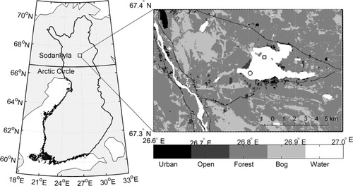
Lake Orajärvi (67.36N, 26.83E) is located in Sodankylä about 8 km east from the Finnish Meteorological Institute (FMI) Arctic Research Centre, some 120 km north of the Arctic Circle (Fig. 1). The surface area of the lake is 11 km². The average water depth is 4.4 m and maximum depth is 11 m. The ice season lasts 6–7 months (from Nov./Dec. to May/June), and the maximum ice thickness usually reaches more than 50 cm in late April, just before the onset of ice melt. Snow is present on the ice surface every winter season but its spatial distribution is variable across the lake.

Fig. 1 Geography map of Lake Orajärvi in Sodankylä. The symbols in the right panel: ○: regular snow and ice thicknesses measurement site; □: SIMB site and, *: Sodankylä weather station.

2.2. Manual measurements

Snow and ice thicknesses have been measured on Lake Orajärvi since the winter season 2009/2010. The measurements are made every second week when the ice is thick enough (for safety reasons), usually through Nov. to April, at approximately the same three sites on the lake. The measurement sites are located at a distance of 400 m from the closest shore and 200 m from a snow mobile route crossing the middle of the lake (Fig. 1). The measured variables are snow and ice thickness (total ice and granular ice), freeboard (the height difference between the ice surface and the water level) and ice layering. The measurements follow the standard procedures of the Finnish Environmental Institute. In addition, a snow pit with profiles of snow grain size, temperature, density and layer structure is recorded at one of the three sites each time.

When ice is formed but still thin, heavy snowfall events may result in flooding, formation of a slush layer and re-freezing to snow ice. However, if the early winter is very cold and ice gets thick rapidly, the snow load may not be heavy enough to create slush, and the insulation effect of snow will reduce the ice growth from the ice bottom. To fully detect these processes, one would need to install a monitoring system, initially in the open water, to measure the ice formation and growth as well as snow accumulation. Unfortunately, such a system is not yet available.

The snow and ice thickness showed striking inter-annual differences in early winter compared to those in later spring (Fig. 2). For example, the ice thickness was 24–39 and 14 cm in early Dec., that is, Julian day (JD) 341 (7 Dec.), JD 343 (9 Dec.) and JD 342 (8 Dec.) in 2009, 2010 and 2011, respectively, and the corresponding snow thickness was 5, 14 and 6 cm, respectively.

Fig. 2 Measurements of mean snow (red) and ice thickness (blue), and freeboard (black) on Lake Orajärvi for: (a) 2009/2010; (b) 2010/2011; and (c) 2011/2012 winter seasons.

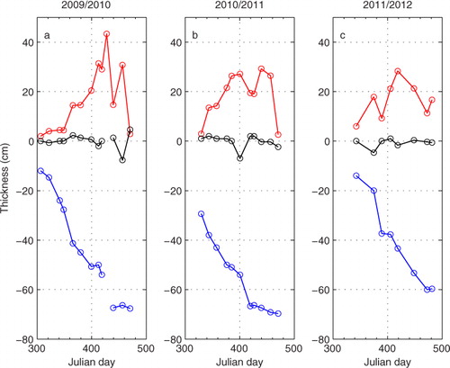
In winter 2010/2011, the thicker ice in the early winter season was most probably formed due to the combined effects of lack of snowfall and very low temperatures during the early winter. These three winter seasons demonstrated that once the freeboard is negative (flooding), it is followed by an increase in ice thickness due to snow–ice formation. In mid-winter, the decrease in snow thickness is correlated with an increase in ice thickness. The ice thickness reaches its maximum value toward the end of the season (late April) before melt starts.

Unfortunately, we have in situ observations neither on ice thickness during the melting seasons nor on the break-up dates in Lake Orajärvi. The break-up dates observed by the Finnish Environmental Institute on Lake Unari, located some 50 km southwest of Lake Orajärvi, are JD 507 (22 May), JD 505 (20 May) and JD 510 (25 May) for these winter seasons, respectively (shown in Fig. 7 as a reference). The area of Lake Unari is 29 km², almost three times that of Orajärvi, but there is a large island in the middle and many small inlets. The maximum water depth is 20 m for Lake Unari and 11 m for Lake Orajärvi, but the average depth of the two lakes is the same within 1 m.

2.3. Buoy observations

In order to make long-term sustainable snow and ice measurements, a prototype ice mass balance buoy developed by the Scottish Association for Marine Science (SAMS) was tested in winters 2009/2010 and 2011/2012. The SAMS Ice Mass Balance Buoy (SIMB) consists of a high-resolution ice thermistor chain (2 cm sensor interval with a total of 240 sensors); data logger compartment; a GPS and iridium data transmission board; flush memory data card and high-capacity alkaline batteries. The SIMB measures the vertical temperature profile from water through ice and snow up to the air. In addition, the SIMB is equipped with heating elements to run a 1–2 minute long heating cycle mode once a day.

The air/snow interface can be identified based on the fact that a number of sensors located in the air have approximately the same temperature (i.e. vertical temperature gradient is small). Based on the same principle, the sensors located in water yield similar temperatures near the bottom of the ice. The snow/ice interface location can be estimated by investigating the temperature perturbations due to the sensor heating. In air, the heating cycles lead typically to a temperature rise of 2°C, in ice and water the typical value is about 0.2°C at least (Jackson et al., 2013). Additionally, since the heat conductivities of snow and ice are different, the temperature gradients in snow and ice are expected to be different. Piecewise linear temperature profiles in snow and ice can, accordingly, be measured during cold conditions. The evolution of snow and ice thickness can finally be inferred based on all these analyses. The SIMB was designed for Polar ocean deployment. This is the first time that the system was deployed in an Arctic lake in Finland.

The Orajärvi test trial in winter 2009/2010 was not a complete success. The measurements suffered from sensors malfunction from time to time and only partial vertical temperature profiles were obtained. After some major technical innovations and software updates, the SIMB was re-deployed in winter 2011/2012 and successfully operated through the whole winter season. At the time of the initial deployment (19 December 2011), the snow thickness was 16 cm and ice thickness was 14 cm, and lake water flooding occurred. The SIMB operated continuously until 13 April 2012 before it was recovered. In addition to regular snow and ice measurements (Fig. 2c), measurements were made when the buoy was visited four times for recording the snow thickness and once for ice thickness (Fig. 3b) before the SIMB was recovered.

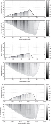
Fig. 3 (a) The SIMB measured snow and ice temperature fields. The number of sensors counts downward from surface to bottom. The snow/ice interface is marked as a black line. (b) SIMB data derived snow and ice thicknesses applying snow/ice interface as zero reference level. The symbols are snow and ice thicknesses measured near the SIMB site (▴) and at regular measurement sites (○).

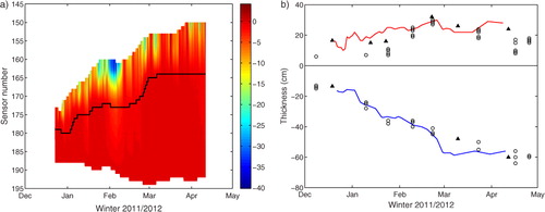
Figure 3 shows SIMB measured snow and ice temperatures and thicknesses. For clarity, we plot temperature in snow and ice only, not showing air and water temperatures. The evolving upper and lower boundaries in Fig. 3a represent the evolution of the snow surface and ice bottom along the thermistor sensor string. The figure also shows the evolution of granular ice thickness: in the beginning of January sensor 180 was in snow, but at the end of the campaign it was 32 cm below the snow/ice interface, indicating the accumulated thickness of snow ice and superimposed ice (the observations do not allow distinguishing between them). The detected maximum bottom ice growth was about 12 cm (distance between sensor 194 and 188) during the SIMB deployment period. In Fig. 3b, the snow/ice interface is set as a reference level to account for the thickness of snow and ice. The independent in situ snow and ice thickness measurements are plotted in Fig. 3b for comparison. The agreement is reasonably good, especially for the ice thickness evolution Mean Bias Error (MBE=1.7 cm). The agreement between the SIMB-based snow thickness evolution and the regular in situ measurements is not as good (MBE=− 6.7 cm) most probably due to the spatial differences of snow distribution (c.f. Fig. 2). However, for the measurements near the SIMB site, the agreement is better (MBE=−0.7 cm).

We need to emphasise that the absolute air-snow and ice-water interfaces can be estimated reasonable well by looking at the thermistor temperature readings. The large uncertainty comes from the detection of the snow–ice interface. Any inaccuracy from this interface detection will eventually affect the snow and ice thickness estimation because we use it as a reference level. One could consider placing a segment (e.g. 20 cm) of the thermistor string horizontally at the ice surface during the SIMB deployment. A clear mark of the initial snow–ice interface location would minimise the error in snow–ice interface detection later on.

2.4. Satellite observations

Space-borne LIST observations from the Moderate Resolution Imaging Spectroradiometer (MODIS) aboard the Terra and Aqua satellites operated by NASA (http://modis.gsfc.nasa.gov) were derived for comparison of the in situ observed and HIGHTSI-simulated snow/ice surface temperatures during the ice season. MODIS day-time and night-time observations at 1 km spatial resolution were utilised. For Lake Orajärvi, MODIS overpass times are mostly between 10:00–12:00 and 20:00–22:00 for both ascending and descending modes. In the case of overlapping acquisition times between the Aqua and Terra satellites, the observations were averaged. MODIS data were processed through an algorithm developed at the University of Waterloo (UW-L3 data, see Kheyrollah Pour et al., 2012, 2014, for details). For Lake Orajärvi, there were about 12 such pixels available that were not contaminated by the surrounding land area. A single (1 km by 1 km) pixel was selected, centred on the location where the in situ (buoy) temperature measurements were made during the study period (2009–2012) to represent the lake surface skin temperature within the hour of in situ observations. MODIS observations are available only during clear-sky conditions, due to the limitation of optical sensors during cloudy days. The time series of MODIS LIST observations for the pixel of interest is compared with the SIMB and HIGHTSI model results (see Section 5.1 below).

Note that although MODIS observations were included in the optimal interpolation surface analysis in the HIRLAM experiment NHFLAK (Kheyrollah Pour et al., 2014), they did not directly influence the HIRLAM forecasts, which were applied as atmospheric forcing data for HIGHTSI in the present study. This is because, in this HIRLAM experiment, the lake surface state was provided by Freshwater Lake (FLake) parameterisation during the atmospheric forecast (see Rontu et al., 2012, for further explanation of relations between analysed and predicted lake variables in HIRLAM). This means that our HIGHTSI results were not influenced by the MODIS observations even indirectly via the atmospheric forcing, hence the MODIS temperatures can be used as independent observations for the evaluation of LIST simulated from HIGHTSI and for comparison with in situ observations.

3. Thermodynamic snow and ice model

A high-resolution thermodynamic snow and ice model was used to calculate the evolution of snow and ice thicknesses. The HIGHTSI model was initially used to calculate seasonal snow and sea ice thermodynamics (Launiainen and Cheng, 1998; Vihma et al., 2002; Cheng et al., 2003, 2006, 2008). The model has been further developed to investigate snow and ice thermodynamics in lakes (Semmler et al., 2012; Yang et al., 2012, 2013).

The snow and ice temperature regimes are solved by the partial-differential thermal heat conduction equations applied for snow and ice layers, respectively. The surface temperature is defined as the upper boundary condition solved by the Norton iterative method from a detailed surface heat/mass balance equation. The turbulent surface fluxes are parameterised taking the thermal stratification of the atmospheric surface layer into account. Downward short- and longwave radiative fluxes are either parameterised, taking into account cloudiness, or prescribed by observations or NWP model output. The penetration of solar radiation into the snow and ice is parameterised according to surface albedo, and optical properties of snow and ice. The surface temperature is also used to determine whether surface melting occurs. At the lower boundary, the ice growth/melt is calculated on the basis of the difference between the ice-water heat flux and the conductive heat flux in the ice. At the snow–ice interface, the snow-to-ice transformation processes through re-freezing of flooded lake water or melted snow are considered in the model (Saloranta, 2000; Cheng et al., 2003).

In the HIGHTSI model, we deal with snow (thickness h _s ), slush, snow/ice (thickness H _si ), superimposed ice (thickness H _su ), columnar ice (thickness H _i ), and lake water. The snow thickness is affected by precipitation, snow melting and flooding slush (thickness h _sL ) formation. The density of snow (ρ _s ) is parameterised according to Anderson (1976). The slush is formed by lake water flooding slush (thickness h _sL ) and snow melting. The density of slush (ρ _sL ) is calculated as a function of density of snow, ice (ρ _i ) and water (ρ _w ) (Saloranta, 2000), and its value is very close to that of water density. Snow–ice is formed by refreezing of flooding slush. The flooding slush is a result of isostatic imbalance of overload snow on top of total ice floe. The superimposed ice is formed via refreezing of melt water or rain. For fresh lake water, we assume that the densities of snow–ice (ρ _si ) and superimposed ice (ρ _su ) are the same and remain constant. The total ice floe is composed of freezing lake water (columnar ice) and formation of snow–ice and superimposed ice (granular ice). The ice and water densities are constants. The freeboard is defined as the distance between the ice surface and water level. When the freeboard tends to be negative, the flooding slush starts to form, and in freezing conditions it is transformed to snow–ice. Table 1 shows the calculation of freeboard and new slush formation in terms of different snow/ice compositions. The melting slush is created by surface and sub-surface snow melting and this part of slush is allowed to be re-frozen to create superimposed ice before the onset of ice melt. For the sake of simplicity, snow–ice and superimposed ice are assumed to form at snow–ice interface (Saloranta, 2000; Cheng et al., 2003; Semmler et al., 2012). For lake conditions, the snow–ice and superimposed ice can be regarded as the same kind of meteoric ice since they both are formed by fresh water, but for sea conditions, the snow–ice is different from superimposed ice because it is formed by salty slush. The formation of a slush layer due to heavy snow load needs water paths, which may consist of thermal cracks or drilling holes.

Table 1. Calculation of freeboard in terms of various snow/ice compositions present in lake

;;	Ice/water
;	Snow, ice/water
;; ;	Snow, flooding slush and ice/water
;; ;	Snow, snow–ice and ice/water
;; ;	Snow, flooding slush, snow–ice and ice/water

B is the buoyancy; ws is the total snow water equivalent in (m). H _sLn is the new slush formation.

If the conductive heat flux at the ice bottom is larger (smaller) than the heat flux from the lake, the ice grows (melts) from the bottom. In this study, the heat flux from the lake was prescribed to a small value of 1.5 W/m² for the freezing season, increasing to 5 W/m² after the onset of ice melt, because penetrating solar radiation heats the lake water below ice.

4. Modelling strategy

4.1. Atmospheric forcing

In this study, local weather station observations and NWP model HIRLAM forecasts were applied as atmospheric forcing for the HIGHTSI experiments.

4.1.1. Weather station data.

The weather station nearest to the lake was located at the FMI Arctic Research Centre, about 8 km from Lake Orajärvi. Due to the distance, the conditions over the lake were not necessarily identical to those observed at the weather station, but the spatial variations are expected to be small as the terrain is almost flat. From this point of view, the weather station data are as representative as the HIRLAM forecasts with a grid spacing of 7.5–16 km (Section 4.1.2). In any case, the variability of weather conditions in the region is dominated by synoptic-scale patterns. The variables measured at the weather station consisted of 10-minute averages of 2-m air temperature (T _a , measured with a PT100 sensor), relative humidity (Rh, Vaisala HMP45D sensor), and 10-m wind speed (V _a , Vaisala WAA25 sensor). The total cloudiness (CN) was measured by a laser ceilometer (Vaisala CT25K), and daily total precipitation (PrecT) was measured by a Vaisala all-weather precipitation gauge VRG101. The downward global shortwave (Q _s ) and longwave (Q _l ) radiative fluxes were measured with Kipp & Zonen CM11 pyranometers and pyrgeometers. All the original measurements were averaged to hourly values and used as external forcing for the ice model. Snow accumulation on land was measured using a Campbell SR50 automatic snow depth sensor every 10 minutes. The data were then averaged to daily means. Snow thickness on land showed large inter-annual variations. The snow season began on JD280 (7 Oct), JD297 (24 Oct) and JD 321 (17 Nov.) for winters 2009/2010, 2010/2011 and 2011/2012, respectively. The corresponding snow-season-average snow thicknesses were 45, 39 and 53 cm and the snowmelt onset dates were JD 454 (30 Mar.) 2010, JD 457 (2 Apr) 2011 and JD 478 (23 Apr) 2012. Table 2 shows the observed seasonal average weather station data for the three winters. For the ice growth season (Nov. to April), striking inter-annual differences are seen in the air temperature, longwave radiation and precipitation. In May and June, in addition to these variables, the wind and shortwave radiation also differ inter-annually.

Table 2. The seasonal (Nov.–Apr.) mean values of observed weather data as well as Bias, Root Mean Square Error (RMSE) and correlation coefficient (R) between hourly time series of HIRLAM forecasts and in situ observed wind, temperature, humidity, downward shortwave and longwave radiation and precipitation for winters 2009/2010; 2010/2011; and 2011/2012

Winter	V a (m/s)	T a (°C)	Rh (%)	Q s (W/m^2)	Q l (W/m^2)	Precipitation total (mm)				Precipitation snow (mm)
09/10	Mean (Nov.–Apr.)	2.3	−9.2	86	42	250	Sum		192		Sum		168
10/11	2.3	−10.4	85	46	237	(Nov.– Apr.)		131		(Nov.– Apr.)		110
11/12	2.3	−6.8	87	41	261	271		218
09/10	Bias (Cal –Ob.)	1.1	−0.2	12.8	−9.8	−6.3	(Nov.–Apr.)		99		(Nov.–Apr.)		67
10/11	0.5	−0.3	7.3	−8.6	−2.2	18		4.8
11/12	0.8	−0.1	6.4	−8.1	−4.5	32		5.3
09/10	RMSE	1.7	3.4	18.2	69.3	24.4
10/11	1.2	3.7	14.2	74.5	22.6
11/12	1.3	3.5	13.4	67.5	30.2
09/10	Corr.	0.78	0.94	0.29	0.74	0.89	h	0.64	d	0.83	h	0.66	d	0.85
10/11	Coeff.	0.77	0.93	0.60	0.74	0.88	0.45	0.68	0.51	0.74
11/12	R	0.78	0.92	0.48	0.73	0.81	0.58	0.82	0.59	0.82

The correlation coefficient (R) between time series of hourly (h) and daily (d) accumulated HIRLAM and in situ observed total and snow precipitations are given.

4.1.2. HIRLAM forecasts.

The HIRLAM NWP model forecasts were utilised in this study as atmospheric forcing. HIRLAM is a short-range NWP model (Undén et al., 2002) developed by an international consortium of 11 European countries (http://hirlam.org). Forcing fields for the first winter (2009/2010) were extracted from the operational HIRLAM archive (3 and 6 hours forecasts, see below). The operational model applied version 7.2, with the standard surface data assimilation and four-dimensional atmospheric data assimilation. A horizontal resolution of 15 km and 60 levels in vertical were used, with the lowest model level centred at 32 m. For winters 2010/2011 and 2011/2012, dedicated HIRLAM model runs were performed for a northern domain (experiment NHFLAK Kheyrollah Pour et al., 2014). These experiments were run with the HIRLAM version 7.4 including renewed surface parameterisations and the FLake parameterisation on lakes. The model resolution was 7 km/65 levels, with the lowest model level centred at the height of ca. 12 m. The lateral boundary conditions for the HIRLAM experiments were obtained from ECMWF analyses, but for the operational HIRLAM of winter 2009/2010 they were derived from ECMWF forecasts. From the three-dimensional HIRLAM output, the lowest model level wind speed (V _a ), air temperature (T _a ) and relative humidity (Rh) were extracted for the grid point nearest to Lake Orajärvi using 3-hour forecasts. Snow precipitation as well as the downward shortwave (Q _s ) and longwave (Q _l ) radiative fluxes were averaged during the first 6-hour forecasts, and taken to represent the conditions at the same time as the extracted temperature, humidity and wind. All values were linearly interpolated to 1-hour interval for the input of ice model experiments. Note that we did not use the diagnostic 2-m temperature and humidity, neither the diagnostic 10-m wind for forcing. Thus the model-based atmospheric data represents somewhat larger-scale conditions than the local synoptic observations to which they are compared in the next section.

4.1.3. Comparison of weather station data and HIRLAM forecasts.

Comparisons between in situ measurements and HIRLAM forecasts were made. In the different HIRLAM versions, the lowest model level variables represent average conditions between the surface and ca. 64 m in version 7.2 (winter 2009–2010) and ca. 25 m in version 7.4 (winters 2010/2011 and 2011/2012). The profiles of wind speed, temperature and water vapour in the surface layer were calculated accordingly based on the Monin-Obukhov similarity theory. It was essential to use the same formulae (Launiainen, 1995) as applied in HIGHTSI when deriving the turbulent surface fluxes from the HIRLAM model level variables. The results were then compared with the observed 2-m air temperature and humidity, and 10-m wind speed. HIRLAM modelled total and snow precipitations (in water equivalent, WE) were compared with observed values. A threshold temperature of 0.5°C was used to extract snow precipitation (PrecS) from the observed total precipitation (Yang et al., 2012). The monthly mean differences between HIRLAM forecasts and weather station observations are shown in Fig. 4. The seasonal statistical error analyses are given in Table 2 .

Fig. 4 The monthly mean differences between HIRLAM forecasts and weather station observations for wind speed (V _a ), air temperature (T _a ), relative humidity (Rh), total precipitation (PrecT), snow precipitation (PrecS), as well as shortwave (Q _s ) and longwave (Q _l ) radiative fluxes for winters 2009/2010, 2010/2011 and 2011/2012. Note the PrecT has the same y-axis [−20, 40], but for May of 2009/2010, the difference was 127 mm.

In general, the agreement between HIRLAM and observations seems better in 2010/2011 and 2011/2012 than in 2009/2010, especially concerning air relative humidity (Fig. 4h, i, Table 2). Winter 2011/2012 was relatively warm in Sodankylä compared to the other two winters. Errors in air temperature were variable, the monthly biases ranging from −2 to 1.5°C, with the largest cold biases in Nov.– Jan. and the largest warm biases in Feb.–April. Shortwave radiation had a negative bias in every season before May. The total precipitation (PrecT) was overestimated by HIRLAM in 2009/2010, particularly for May. The exact reason for this large bias (127 mm) still remains unknown. In general, the pointwise validation of simulated and observed precipitation in winter time contains uncertainties due to several reasons related to areal representativeness of the measurements and model results as well as to the known problems of snowfall measurement due to wind effect. In this study, however, the bias of PrecT are mostly less than 20 mm WE. In spring, the bias of PrecT is slightly larger (20–30 mm WE). The HIRLAM snow precipitation (PrecS) agrees better with observed values. The biases are mostly well under 20 mm WE. The bias of accumulated snow precipitation (Nov.–Apr.) is much smaller compared with the corresponding accumulated total precipitation indicating that HIRLAM PrecS is pretty reliable for ice modelling. For all seasons, the correlation coefficients between HIRLAM modelled and in situ observed wind speed, air temperature, shortwave and longwave radiative fluxes as well as the daily accumulated precipitation are quite good (Table 2).

Despite the dominance of positive biases in air relative humidity and precipitation, the downward shortwave and longwave radiation were underestimated on average. The new HIRLAM version is known to predict less low clouds in spring than the previous one, which may be reflected in the improved scores in the last two springs for the relative humidity, total precipitation, and shortwave radiation (Fig. 4).

4.2. HIGHTSI experiments

The HIGHTSI experiments are listed in Table 3. The initial snow and ice conditions were set according to the available in situ observations. For each of the three winters, two experiments were performed including the snow pack on lake ice: one forced by the weather station data (SL experiments, c.f. Tab.3) and another by HIRLAM forecasts (SH experiments). Model experiments without snow (L and H) were also carried out. In L and H runs, the external precipitation forcing was set to be zero so the ice growth is purely in response to the weather forcing of wind, temperature, moisture, and cloudiness. The purpose of these model runs was to demonstrate the importance of winter precipitation as external forcing on snow and ice modelling.

Table 3. The names of HIGHTSI modelling experiments

Forcing	2009/2010	2010/2011	2011/2012
with snow
local in situ observation	0910SL	1011SL	1112SL
HIRLAM forecasts	0910SH	1011SH	1112SH
no snow
local in situ observation	0910L	1011L	1112L
HIRLAM forecasts	0910H	1011H	1112H

SL: snow considered with local weather forcing; SH: snow considered with HIRLAM forecasts forcing; L: no snow with local weather forcing; H: no snow with HIRLAM forecasts forcing. The numbers (0910, 1011 and 1112) in front character represent the annual winter seasons.

5. Results

5.1. Surface temperature and energy budget

For the SL modelling experiments, the HIGHTSI simulated surface temperatures were compared with MODIS LIST observations over Lake Orajärvi (Figs. 5 and 6, and Table 4). The coverage of MODIS observations was relatively good in time, with the exception of a few longer cloudy periods. The comparison indicates that under cold conditions, MODIS and HIGHTSI temperatures are of the same order of magnitude. The satellite observations tend to show lower surface temperature during cold dark nights (−2.8°C≤MBE≤−3.9°C). Differences of the same magnitude have been reported by Kheyrollah Pour et al. (2012) in a comparison between MODIS and FLake modelled surface temperatures over several ice seasons (2002–2010) on Great Bear Lake and Great Slave Lake, Northwest Territories, Canada. Under melting conditions in spring, the MODIS surface temperatures are higher than those estimated by HIGHTSI. However, MODIS and HIGHTSI surface temperatures agree better in terms of temporal variation. A summary of the statistical indices is presented in Table 4. In Fig. 5c, SIMB data are also compared with HIGHTSI and MODIS during winter 2011/2012. The cross-comparison is shown in scatterplots in Fig. 6.

Fig. 5 The HIGHTSI (experiments SL, c.f. Table 4) modelled (red line) and MODIS observed LIST (blue dots) for winter (a) 2009/2010; (b) 2010/2011; and (c) 2011/2012. The SIMB measured surface temperature is given as the green line in (c).

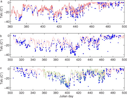
Fig. 6 The comparison of surface temperature: (a) MODIS versus HIGHTSI (SL experiments, c.f. Table 4); (b) MODIS versus SIMB; and (c) HIGHTSI versus SIMB for winter 2011/2012.

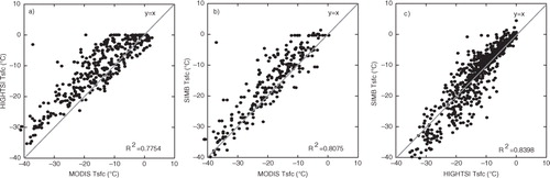
Table 4. Mean Bias Error (MBE), standard deviation (std), Root Mean Square Error (RMSE) and correlation coefficient (R) of HIGHTSI (experiments SL, c.f. Table 3) modelled surface temperature, as well as SIMB and MODIS observations

Winter	Results compared	MBE	std	RMSE	R	n
2009/2010	HIGHTSI–MODIS	2.9	4.5	5.4	0.93	277
2010/2011	HIGHTSI–MODIS	2.8	5.1	5.8	0.89	416
2011/2012	HIGHTSI–MODIS	3.9	4.9	6.5	0.88	375
MODIS–SIMB	−3.1	4.6	5.5	0.9	253
HIGHTSI–SIMB	0.03	2.8	3.8	0.91	757

In most cases, the MODIS surface temperatures were lower than the SIMB measurements and HIGHTSI results during winter 2011/2012 (Fig. 5a, b; Table 4). The agreement between HIGHTSI and SIMB surface temperature is better, particularly during warm conditions (temperature>−10°C). For temperatures lower than −10°C, the HIGHTSI surface temperature was usually higher than SIMB values.

To better understand the inter-annual evolution of snow and ice in Lake Orajärvi, the monthly means for various surface heat fluxes are calculated from 0910SL, 1011SL and 1112SL experiments (Table 5). For a seasonal cycle, the net solar radiation (Q _snet ) remains small before daytime melting season starts in April. The net longwave (Q _lnet ) cooling dominates during the winter season. In early winter the turbulent heat fluxes were small, but when spring came the sensible heat flux increased because of positive air temperatures exceeding the lake surface temperature, which remained at or below 0°C until the ice break-up (the air temperatures were observed over land, but we assume that they will represent conditions over the small lake). The upward conductive heat flux (F _c ) represents the near surface snow/ice temperature gradient. When ice was thin, the larger F _c indicates more heat lost from the ice bottom to the snow surface and, as a results, greater ice growth. The net surface heat flux (F _net ) indicates the overall heat gain and loss of the surface layer. In early winter, the heat gain of the surface layer results from rapid ice growth at ice bottom. In late spring, the heat gain of the surface layer results from strong solar heating (i.e. surface melting starts).

Table 5. HIGHTSI (experiments SL, c.f. Table 3) modelled monthly mean surface heat fluxes for three winter seasons. Q _snet : net shortwave radiative flux at surface; Q _lnet : net longwave radiative flux; Q _h : sensible heat flux; Q _le : latent heat flux; F _c : surface conductive heat flux; F _net : net surface heat flux, that is, the sum of Q _snet , Q _lnet , Q _h , Q _le and F _c . All fluxes are positive toward surface (heat gain)

Q snet	Q lnet	Q h	Q le	F c	F net
Year	Month	W/m^2
09/10	11	0.1	−5.7	1.1	−0.6	6.9	2.0
12	0.01	−19.4	2.2	−0.01	21.4	4.2
01	0.12	−17.9	1.9	−0.9	19.5	2.8
02	2.2	−17.9	−4.2	−1.7	16.8	−4.8
03	9.0	−35.0	5.6	−1.8	13.9	−8.3
04	11.4	−29.6	10.4	−3.2	13.3	2.2
05	23.9	−7.3	12.4	4.4	9.9	43.3
10/11	11	0.2	−29.2	0.1	−0.6	40.2	11.0
12	0.01	−23.8	−1.6	−1.0	34.3	8.0
01	0.16	−19.1	1.8	−0.02	21.1	4.0
02	2.3	−22.8	−1.6	−0.9	18.1	−5.1
03	9.3	−43.7	14.7	−1.7	13.4	−8.0
04	13.5	−31.2	12.7	−1.8	12.4	5.7
05	26.9	−17.4	18.2	3.9	7.8	30.9
11/12	11	0.4	−15.9	3.9	2.2	9.1	−0.3
12	0.01	−11.9	5.2	1.1	8.8	3.3
01	0.26	−10.6	−1.1	−1.6	10.4	−2.5
02	2.5	−15.9	−1.0	−1.3	10.6	−5.0
03	11.2	−34.6	9.3	0.8	8.6	−6.3
04	20.9	−30.6	5.9	−2.4	7.1	0.9
05	25.9	−27.3	24.7	−0.1	7.3	30.5

The surface energy balance in early winter 2010/2011 differed from the other seasons. The strong longwave cooling (Table 4), associated with large F _c created rapid ice growth in early winter (note that the F _net in Nov.–Dec. was almost 2–3 times larger than other seasons). The modelled ice thickness (c.f. Fig. 7), described in the next section, indeed shows thicker ice in mid-Dec. (JD350) of 2010/2011 season compared with other seasons. Comparing the surface energy budget of 2009/2010 against 2011/2012, we see that in 2011/2012 the net surface heat flux F _net was smaller than in 2009/2010, which may be partly explained by slightly thinner ice in winter 2011/2012. In May, the smaller heat gain by the surface layer may have resulted in slower surface melting and consequently delayed break-up for winter 2011/2012.

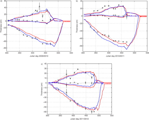
Fig. 7 HIGHTSI modelled snow thickness (upper lines), ice thicknesses (lower lines) and freeboard (middle lines) compared to in situ observations for 2009/10 (a), 2010/11 (b) and 2011/12 (c). The zero reference level is the snow–ice interface. The model runs were based on atmospheric forcing from weather station data (red lines) and HIRLAM forecasts (blue lines). The observations are given as black circles and their standard deviations are marked as vertical bars. The observed ice break-up dates of Lake Unari are indicated by red circles.

5.2. Snow and ice evolution

The time series of modelled snow and ice thickness as well as freeboard are presented in Fig. 7. For winter 2009/2010, snow was modelled well until JD400 (4 Feb.) for experiments 0910SL and 0910SH. The large variations in snow depth between days JD400 (4 Feb.) and JD450 (26 Mar.) were not well captured by the model owing to the failure to capture the large snowfall between JD418 (22 Feb.) and JD427 (3 Mar.). The modelled timing of snowmelt onset agreed well with observations but the melting rates were slower than observed. The differences between modelled snow thickness in 0910SL and 0910SH were large in Dec. and Mar. Although, the HIRLAM total accumulated snow precipitation has a 67 mm positive bias during the season (Fig. 4), a cold HIRLAM T _a bias and smaller Q _l made 0910SH produce thicker ice.

For winter 2010/2011, the bias of HIRLAM seasonal accumulated snow precipitation was only 4.8 mm; therefore the 1011SL and 1011SH modelled snow thicknesses were close to each other. Again, the large errors of modelled snow thickness occurred during rapid snowfall period from JD329 (25 Nov.)–JD 343 (9 Dec.). The 1011SH produced more ice than 1011SL towards the end of the March (JD450); the difference between modelled ice thicknesses actually started already in the early season (Nov.) due to too-small Q _l and a large cold bias in HIRLAM.

For winter 2011/2012, the modelled snow accumulations in SL and SH experiments were improved compared with results of previous winter seasons. The maximum observed snow thickness was often underestimated. The observed snow precipitation was larger than HIRLAM forecasts before March (c.f. Fig. 4o) making the snow pack thicker in 1112SL than 1112SH (although the bias of HIRLAM seasonal accumulated snow precipitation was 5.7 mm due to the compensation effect). In this winter, the first snow-day on land was late, that is, 17 Nov. versus 7 and 24 Oct. for the two other winters. However, the SL and SH gave quite similar ice growth in early Nov. because of no snow on ice. The difference of SL and SH modelled ice thickness in the rest of the season was due to the appearance of snow in SL and SH experiments and differences in other weather forcing variables.

For each spring, the snowmelt onset dates calculated by SL and SH experiments were close to each other. Compared to the observed snowmelt onset on land, the agreements were very good, that is, 30 March (observed) versus 1 April (calculated) for 2009/2010, 2 April (both observed and calculated) for 2010/2011, and 23 April (both observed and calculated) for 2011/2012. The earlier onset of modelled snow melt was consistent with the earlier modelled breakup date.

The validation of freeboard modelling is a challenge. In this study, the rapid change of freeboard was often underestimated. In HIGHTSI, the freeboard is calculated according to Table 1. In reality when snow is flooded, the lake water maybe merged upward due to the capillarity suction effect. We were not able to consider this micro scale process in HIGHTSI. On the other hand, HIGHTSI reproduced reasonably well the transformation of snow to ice; the model experiments revealed that the total ice formation would be largely underestimated if freezing is allowed only at the ice bottom (c.f. Table 6).

Table 6. The seasonal maximum ice thickness (H _imax ), ice bottom growth and percentage of snow to ice transformation for SL and SH experiments and H _imax for L and H experiments for three ice seasons

2009/2010	2010/2011	2011/2012
SL	H imax (cm)	66	81	57
SH	75	89	55
SL	Columnar ice (cm)	36	56	27
SH	39	67	31
SL	Granular ice (%)	46	30	53
SH	48	24	44
L	H imax (cm)	120	132	96
H	123	135	99

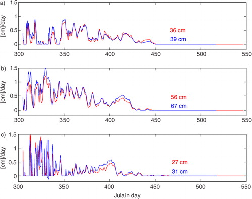
The modelled maximum ice thicknesses as well as accumulated ice bottom growth (columnar ice) and percentage of snow to ice transformation (granular ice) for the three winters are given in Table 6 for the SL and SH experiments. For SL experiments, the bottom growth (Fig. 8) lasted until 26 March in winter 2009/2010, but the ice thickness increased mainly during early winter (Dec.–Jan.). For winter 2010/2011, the pronounced bottom growth occurred until 1 March followed by a slight thickness increase until 26 March, but most of the growth occurred between Nov. and early January. For winter 2011/2012, the bottom growth was more significant in Nov. and early Dec. Afterwards, it slowed down until 14 Feb. and continued with a very small increase until 6 March, which was in good agreement with the SIMB measurements (Fig. 3). The bottom ice growth for the SH experiments showed similar variation compared to SL experiments for winters 2009/2010 and 2010/2011. For winter 2011/2012, the SH run produced more bottom growth than the SL run. During the cold winter 2010/2011, snow precipitation was small and ice growth mainly took place at the ice bottom, whereas for the mild winter 2011/2012, the majority of ice growth was due to snow–ice and superimposed ice formation.

Fig. 8 The HIGHTSI modelled ice bottom growth for (a) 0910SL (red) and 0910SH (blue); (b) 1011SL (red) and 1011SH (blue); and (c) 1112SL (red) and 1112SH (blue).

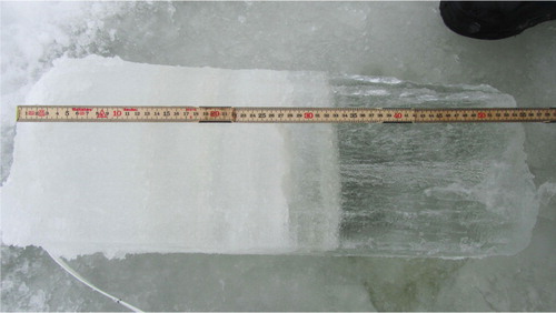
An ice core sample collected on 12 April 2012 (Fig. 9) indicated the total ice thickness was about 57 cm, of which 24 cm (42%) was columnar ice and 33 cm (58%) was granular ice (snow–ice and superimposed ice). Compared to the initial deployment of the SIMB on 19 Dec. 2011, when the ice thickness was 14 cm, the ice bottom growth until 12 April 2012 was 10 cm, which is in line with the SIMB detection (see Section 2.3, Fig. 3a). The 1112SL experiment yielded total ice thicknesses in good agreement with the observations during the growth season, and the observed and modelled maxima occurred within 5 d of each other.

Fig. 9 Ice core sample collected on 12 April 2012 when the SIMB was recovered.

The modelled snow and ice temperature fields for SL experiments (Fig. 10) revealed that the snow–ice interface remained cold during the winter season, which ensured freezing of slush to form snow–ice. After the snowmelt onset, the ice surface temperature was also low, leading to re-freezing of surface snowmelt to form superimposed ice.

Fig. 10 HIGHTSI (SL experiments, c.f. Table 3) modelled snow and ice temperatures for winter seasons 2009/2010, 2010/2011, and 2011/2012. For the sake of clarity, snow and ice temperatures have the same vertical scales but different temperature grey scales.

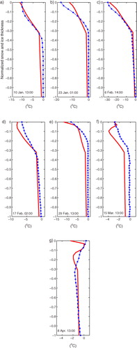
The modelled and observed vertical snow and ice temperature profiles at selected time steps are shown in Fig. 11. Considering the surface temperature, the large discrepancy between observations and model results on 23 Jan. (Fig. 11b) was associated with inaccuracy of the SIMB snow thickness (Fig. 3b). Under cold conditions, the snow and ice temperatures were modelled quite well. With warm conditions, the modelled and observed temperature differences in snow and ice were larger. This could be due to the error of modelled snow thickness as well as the unknown effect of solar transmission into snow and ice. The agreement between modelled and observed temperature was better in ice than in snow. On 8 April, sub-surface melting was captured by the model run (Fig. 11g). The SIMB observations did not detect this phenomenon, but showed temperatures increasing towards the surface, with erroneous positive values due to solar heating of the sensors.

Fig. 11 The comparison of 1112SL modelled (red line) and SIMB observed (dot-blue line) vertical temperature profiles within snow and ice at selected UTC time steps. A normalized coordinate, that is, height/(h _s +H _i ) is used in the y-axis (0 is surface and 1 is ice bottom).

5.3. Lake ice simulations using different precipitation scenarios

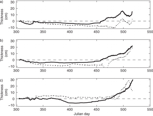
Precipitation introduces a large uncertainty on snow and ice evolution in a lake. The uncertainty originates not only from the strong snow insulation effect, but also from the intensity and timing of snowfall associated with the synoptic-scale patterns and hydrostatic imbalance between snow cover and underlying ice floe. To demonstrate the uncertainty related to precipitation forcing, we carried out a few model experiments without snow. We used the same initial ice thickness (0.01 m) for each L and H experiments, which all covered the period from the beginning of Nov. to the end of May. For each winter season, L and H modelled ice thickness (Fig. 12) yielded a fairly similar ice evolution. For each season, the modelled maximum ice thicknesses in L and H experiments were close to each other (Table 6), whereas for SL and SH experiments the seasonal maximum ice thicknesses differed from each other. The differences of modelled ice thickness between SL and SH and L and H experiments are shown in Fig. 13. The differences between modelled ice thickness using in situ and HIRLAM forcing without snow are much smaller than the corresponding differences between model experiments with snow taken into account, particularly in early winter season (Nov.–Dec.). This demonstrates the central role of the uncertainty in precipitation forcing. During the melt season, the differences of modelled ice thickness between SL and SH and L and H are getting large. These differences are partly due to differences in radiative forcing. Compared to in situ observations, the monthly mean HIRLAM longwave radiative fluxes were 7–10 W/m² smaller during the winter months (Nov.–Feb.) and 3–5 W/m² larger in spring (March–May). The HIRLAM shortwave radiative fluxes were 4–7 W/m² larger in spring (March–May).

Fig. 12 HIGHTSI modelled ice evolution without taking snow into account, using in situ weather station data (solid line) and HIRLAM forecasts (dotted line) as external forcing. The winter seasons are 2009/2010 (red), 2010/2011 (black), and 2011/2012 (blue).

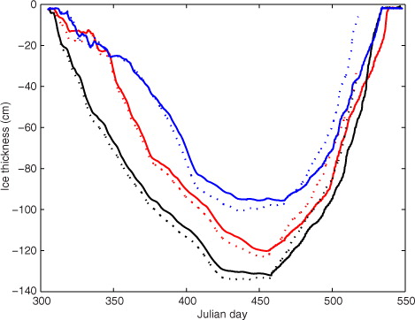
Fig. 13 The differences of modelled ice between model runs (without snow: solid lines; with snow: dotted line) using in situ weather station data and HIRLAM forecasts as external forcing. (a) 2009/2010; (b) 2010/2011; and (c) 2011/2012.

The impact of precipitation is closely linked to formation of snow–ice and superimposed ice (Table 1). The increase of snowfall makes the snow-load heavier, promoting negative ice freeboard, which is the basis for snow–ice formation. Rain and sleet falling on snow favour snow–slush for superimposed ice formation. In winter 2011/2012, for example, a number of model sensitivity experiments indicated that when the snow precipitation was 50% of the original observed value, the maximum ice thickness only increased from 57 to 58 cm, but the proportions of granular and columnar ice changed a lot: from 53 to 20% for granular ice and from 47 to 80% for columnar ice. If the snow precipitation increased to 1.5 times of its original value, while keeping all other forcing factors equal, the model run ends up with 66 cm maximum ice thickness and the proportions of granular and columnar ice were 71 and 29%, respectively. We emphasise that these proportions are strongly associated with precipitation patterns as well as variations in air temperature during the winter season. The sensitivity tests merely demonstrated the impact of snow precipitation on granular and columnar ice formation. A more in-depth investigation would have required a large number of model runs taking into account different combinations of external forcings. This is a topic that we plan to pursue in a follow-up study.

6. Conclusions

The evolution of snow and ice temperature, thickness and energy balance in Lake Orajärvi was investigated during three successive winter seasons (2009–2012). A prototype ice mass balance buoy (SIMB) was deployed to monitor snow and ice temperature profiles and thicknesses. The evolution of snow and ice in Lake Orajärvi was simulated by HIGHTSI model with external forcing data from in situ weather station observations and HIRLAM NWP model forecasts. The performance of HIRLAM forecasts was assessed against weather station observations. The HIGHTSI results were validated using lake snow and ice measurements.

Our successful deployment of the SIMB buoy and data analyses suggest that this system is a reliable instrument set-up for monitoring snow and ice temperatures and thicknesses in an Arctic lake. The SIMB-based snow and ice thicknesses were in a reasonably good agreement with manual borehole measurements in cold conditions. The SIMB measurements clearly indicated that snow to ice transformation took place at the snow/ice interface. Challenges remain for warm conditions, in particular when the snow and ice are close to isothermal. In such situations, the detection of snow and ice thickness based on the temperature profile is likely to be uncertain. Additionally, the solar heating may cause errors in the readings of the uppermost temperature sensors during the melting season. Although the SIMB is still largely a prototype system for snow and ice monitoring (Jackson et al., 2013), its relatively low cost and compact design make this device competitive. We have also successfully deployed SIMB buoys for snow and ice monitoring also on sea ice in the Arctic, Antarctic, and the Baltic Sea.

MODIS surface temperature observations are a promising data source for optimal interpolation surface analyses in operational NWP (Kalle Eerola, personal communication, 2014). Under clear-sky conditions, space-borne thermal remote sensing data can also be used to retrieve large-scale ice thickness during the growth season (Yu and Rothrock, 1996; Mäkynen et al., 2013). The MODIS snow/ice (skin) surface temperatures were compared to those modelled with HIGHTSI and measured with the SIMB. Compared to simulated and in situ LIST data, MODIS showed 2.8–3.9°C lower temperatures, with the largest differences during cold dark nights. These results are in line with those previously reported by Kheyrollah Pour et al. (2012).

The weather conditions in early winter are critical in determining the seasonal evolution of the thickness of lake ice and snow. During the freezing season, the most important forcing factors that lead to inter-annual variations in lake ice conditions are air temperature, precipitation and net longwave radiative flux. These are the essential external forcing factors for ice growth. A first-order estimate for the effect of air temperature on ice thickness can be obtained from an analytical solution for ice growth (Leppäranta, 1993). Such an estimate, however, does not take in to account the effects of precipitation and the individual terms of the surface energy balance to the snow and ice thickness, which were addressed in this study. Our results for the rate of bottom growth in early winter were comparable to previous studies (Launiainen and Cheng, 1998), being of the order of 1–2 cm day⁻¹. Before ice melt onset, the growth rate of superimposed ice was, however, of the same order of magnitude as the bottom growth in the early winter. The timing of superimposed ice formation agreed reasonable well with in situ observations carried out in a similar snow and ice environment on land-fast ice in the Baltic Sea (Granskog et al., 2006) and in an Arctic fjord (Nicolaus et al., 2003).

The largest external uncertainty originated from precipitation. This was revealed by HIGHTSI experiments in which snow on ice was not taken into account. Without precipitation, the model experiment forced by HIRLAM forecasts and in situ observation yielded very similar seasonal ice evolution in terms of the early season ice growth and the maximum ice thickness. With external forcing including precipitation, the simulated ice thickness differed a lot between the experiments forced by HIRLAM and in situ observations.

Improvements to the HIRLAM NWP model were made by increasing the horizontal and vertical resolution and including the FLake parameterisation. The forcing fields in 2010/2011 and 2011/2012, based on the improved HIRLAM, were indeed better for the relative humidity and solar radiation compared with those in 2009/2010. The HIRLAM weather forcing time series correlated reasonable well with in situ observations of wind speed, air temperature, shortwave and longwave radiative fluxes and daily accumulated total and snow precipitations. The increase of snow depth over lake ice is not easy to model well. Large errors originate from the uncertainty of the external forcing related to the wind impact to the in situ precipitation observations and inaccurate NWP precipitation forecasts. The accuracy of HIRLAM total precipitation, its division between rain and snowfall, as well as prediction of individual precipitation events requires further improvements. Further efforts are also needed to implement in models the recent advances in physics of snow and ice albedo and related feedbacks, effects of aerosol deposition on snow and ice, and transmittance of snow and ice (Vihma et al., 2014).

It is vitally important to include calculation of snow to ice transformation in the lake ice modelling. Ice growth from the bottom accounted only for a portion of the total ice thickness of the lake examined in this study. At the seasonal time scale, bottom growth constituted about 50–70% of the total ice growth; the percentage strongly depends on the amount of total snow precipitation as well as the air temperature regimes.

During the melting season, HIGHTSI modelled ice thickness driven by HIRLAM and by in situ observations tend to differ from each other. The downward shortwave radiative flux and surface albedo play important roles on surface melting. Due to safety regulations, we do not have sufficient in situ observations on lake ice for investigation of the lake ice melting process. Although HIGHTSI reproduced well the observed timing of snow melt onset, the redistribution of melting water runoff rather than to re-freezing remains unknown and needs to be investigated in the future. We also expect further development of SIMB to improve the accuracy and reliability of the observations during melting seasons.

7. Acknowledgements

The in situ measurements on Lake Orajärvi were part of the NoSREx (Nordic Snow Radar Experiment) project, funded by the European Space Agency (ESA-ESTEC) Contract No. 22671/09/NL/JA (Technical Assistance for the Deployment of an X- to Ku-band Scatterometer During the NoSREx Experiment). The work of T.V. was supported by the Academy of Finland (contract 259537). Additional support was provided through European Space Agency (ESA-ESRIN) Contract No. 4000101296/10/I-LG (Support to Science Element, North Hydrology Project). The support by the international HIRLAM-B programme is acknowledged.

References

- Anderson E . A Point Energy and Mass Balance Model for a Snow Cover. 1976; NOAA Technical Report. NWS 19, USA, 150 pp.
- Atlaskin E , Vihma T . Evaluation of NWP results for wintertime nocturnal boundary-layer temperatures over Europe and Finland. Q. J. Roy. Meteorol. Soc. 2012; 138: 1440–1451.
- Bosilovich M. G. , Chen J. , Robertson F. R. , Adler R. F . Evaluation of global precipitation in reanalyses. J. Appl. Meteorol. Climatol. 2008; 47: 2279–2299. http://dx.doi.org/10.1175/2008JAMC1921.1.
- Brown L. C. , Duguay C. R . The response and role of ice cover in lake–climate interactions. Prog. Phys. Geogr. 2010; 34: 671–704.
- Brown L. C. , Duguay C. R 2011. The fate of lake ice in the North American Arctic. Cryosphere. 5, 869–892. DOI: 10.5194/tc-5-869-2011.
- Cheng B. , Vihma T. , Launiainen J . Modelling of the superimposed ice formation and sub-surface melting in the Baltic Sea. Geophysica. 2003; 39: 31–50.
- Cheng B. , Vihma T. , Pirazzini R. , Granskog M . Modelling of superimposed ice formation during spring snowmelt period in the Baltic Sea. Ann. Glaciol. 2006; 44: 139–146.
- Cheng B. , Zhang Z. , Vihma T. , Johansson M. , Bian L , co-authors . Model experiments on snow and ice thermodynamics in the Arctic Ocean with CHINAREN 2003 data. J. Geophys. Res. 2008; 113: C09020.
- Duguay C. R. , Brown L. C. , Kang K.-K. , Kheyrollah Pour H . [Arctic]. Lake ice. [In State of the Climate in 2011]. Bull. Am. Meteorol. Soc. 2012; 93(7): 152–154.
- Duguay C. R. , Brown L. C. , Kang K.-K. , Kheyrollah Pour H . [Arctic]. Lake ice. [In State of the Climate in 2012]. Bull. Am Meteorol. Soc. 2013; 94(7): 156–158.
- Duguay C. R. , Flato G. M. , Jeffries M. O. , Ménard P. , Morris K. , co-authors . Ice-cover variability on shallow lakes at high latitudes: model simulations and observations. Hydrol. Process. 2003; 17: 3464–3483.
- Duguay C. R. , Prowse T. D. , Bonsal B. R. , Brown R. D. , Lacroix M. P. , co-authors . Recent trends in Canadian lake ice cover. Hydrol. Process. 2006; 20: 781–801.
- Eerola K. , Rontu L. , Kourzeneva E. , Shcherbak E . A study on effects of lake temperature and ice cover in HIRLAM. Boreal Environ. Res. 2010; 15: 130–142.
- Granskog M. , Vihma T. , Pirazzini R. , Cheng B . Superimposed ice formation and surface fluxes on sea ice during the spring melt–freeze period in the Baltic Sea. J. Glaciol. 2006; 52(176): 119–127.
- Jackson K. , Wilkinson J. , Maksym T. , Meldrum D. , Beckers J. , co-authors . A novel and low cost sea ice mass balance buoy. J. Atmos. Ocean. Tech. 2013; 30(11): 2676–2688.
- Jakobson E , Vihma T . Atmospheric moisture budget over the Arctic on the basis of the ERA-40 reanalysis. Int. J. Climatol. 2010; 30: 2175–2194.
- Kang K.-K. , Duguay C. R. , Howell S. E., Derksen C. P. , Kelly R. E. J . Sensitivity of AMSR-E brightness temperatures to the seasonal evolution of lake ice thickness. IEEE Geosci. Rem. Sens. Lett. 2010; 7(4): 751–755.
- Kheyrollah Pour H. , Duguay C. R. , Martynov A. , Brown L. C . Simulation of surface temperature and ice cover of large northern lakes with 1-D models: a comparison with MODIS satellite data and in situ measurements. Tellus A. 2012; 64: 17614.
- Kheyrollah Pour H. , Duguay C. R. , Solberg R. , Rudjord Ø Impact of satellite-based lake surface observations on the initial state of HIRLAM. Part I: Evaluation of remotely-sensed lake surface water temperature observations. Tellus A. 2014; 66: 21534. DOI: http://dx.doi.org/10.3402/tellusa.v66.21534 .
- Launiainen J . Derivation of the relationship between the Obukhov stability parameter and the bulk Richardson number for the flux-profile studies. Boundary Layer Meteorol. 1995; 76: 165–179.
- Launiainen J. , Cheng B . Modelling of ice thermodynamics in natural water bodies. Cold Reg. Sci. Technol. 1998; 27(3): 153–178.
- Lenaerts J. T. M. , van den Broeke M. R . Modelling drifting snow in Antarctica with a regional climate model: 2. Results. J. Geophys. Res. 2012; 117: 05109.
- Leonard K. , Maksym T . The importance of wind-blown snow redistribution to accumulation on and mass balance of Bellingshausen Sea ice. Ann. Glaciol. 2011; 52(57 Pt 2): 271–278.
- Leppäranta M . A review of analytical sea ice growth models. Atmos. Ocean. 1993; 31(1): 123–138.
- Mäkynen M. , Cheng B. , Similä M . On the accuracy of the thin ice thickness retrieval using MODIS thermal imagery over the Arctic first year ice. Ann. Glaciol. 2013; 54(62): 87–96.
- Morris K. , Jeffries M. , Duguay C. R . Model simulation of the effects of climate variability and change on lake ice in central Alaska, USA. Ann. Glaciol. 2005; 40: 113–118.
- Nicolaus M. , Haas C. , Bareiss J . Observations of superimposed ice formation at melt-onset on fast ice on Kongsfjorden, Svalbard. Phys. Chem. Earth. 2003; 28: 1241–1248.
- Niziol T. A . Operational forecasting of lake effect snowfall in Western and Central New York. Weather Forecast. 1987; 2: 310–321. DOI: http://dx.doi.org/10.1175/1520-0434(1987)0020310:OFOLES2.0.CO;2 .
- Pirazzini R . Challenges in snow and ice Albedo parameterizations. Geophysica. 2009; 45(1–2): 41–62.
- Prowse T. , Alfredsen K. , Beltaos S. , Bonsal B. , Duguay C. R. , co-authors . Changing lake and river ice regimes: trends, effects and implications. AMAP (2011). Snow, Water, Ice, and Permafrost in the Arctic (SWIPA): Climate Change and the Cryosphere.
- Prowse T. D.. , Brown K . Hydro-ecological effects of changing Arctic river and lake ice covers: a review. Hydrol. Res. 2010; 41: 454–461.
- Rontu L. , Eerola K. , Kourzeneva E. , Vehviläinen B . Data assimilation and parameterization of lakes in HIRLAM. Tellus A. 2012; 64: 17611.
- Rouse W. R. , Blanken P. D. , Duguay C. R. , Oswald C. J. , Schertzer W. M , Woo M. K . Climate lake interactions. Cold Region Atmospheric and Hydrologic Studies: The Mackenzie GEWEX Experience. 2008; Springer, Berlin. 139–160.
- Saloranta T . Modelling the evolution of snow, snow ice and ice in the Baltic Sea. Tellus A. 2000; 52: 93–108.
- Semmler T. , Cheng B. , Yang Y. , Rontu L . Snow and ice on Bear Lake (Alaska)–sensitivity experiments with two lake ice models. Tellus A. 2012; 64: 17339.
- Surdu C. M. , Duguay C. R. , Brown L. C. , Fernández Prieto D . Response of ice cover on shallow lakes of the North Slope of Alaska to contemporary climate conditions (1950–2011): radar remote-sensing and numerical modelling data analysis. Cryosphere. 2014; 8: 167–180.
- Tjernström M. , Sedlar J. , Shupe M. D . How well do regional climate models reproduce radiation and clouds in the Arctic? An evaluation of ARCMIP simulations. J. Appl. Meteorol. Climatol. 2008; 47: 2405–2422.
- Undén P. , Rontu L. , Järvinen H. , Lynch P. , Calvo J. , co-authors . The HIRLAM-5 Scientific Documentation. 2002; 144. Online at: http://hirlam.org and SMHI, S-60176 Norrköping, Sweden.
- Vihma T. , Pirazzini R. , Renfrew I. A. , Sedlar J. , Tjernström M. , co-authors . Advances in understanding and parameterization of small-scale physical processes in the marine Arctic climate system: a review. Atmos. Chem. Phys. Discuss. 2014; 13: 32703–32816.
- Vihma T. , Uotila J. , Cheng B. , Launiainen J . Surface heat budget over the Weddell Sea: buoy results and comparisons with large-scale models. J. Geophys. Res. 2002; 107: C2.
- Walsh J. E. , Anisimov O. , Hagen J. O. M. , Jakobsson T. , Oerlemans J. , co-authors . Symon C. , Arris L. , Heal B . Cryosphere and hydrology. Arctic Climate Impact Assessment. 2005; , Cambridge: Cambridge University Press. 183–242.
- Wright D. M. , Posselt D. J. , Steiner A. L . Sensitivity of lake-effect snowfall to lake ice cover and temperature in the great lakes region. Mon. Weather Rev. 2013; 141: 670–689. http://dx.doi.org/10.1175/2008JAMC1921.1.
- Yang Y. , Cheng B. , Kourzeneva E. , Semmler T. , Rontu R. , co-authors . Modelling experiments on air–snow–ice interactions over a high Arctic lake. Boreal Environ. Res. 2013; 18: 341–358.
- Yang Y. , Leppäranta M. , Cheng B. , Li Z . Numerical modelling of snow and ice thickness in Lake Vanajavesi, Finland. Tellus A. 2012; 64: 17202.
- Yu Y. , Rothrock D. A . Thin ice thickness from satellite thermal imagery. J. Geophys. Res. 1996; 101(C10): 25753–25766.