Improving quantitative precipitation nowcasting with a local ensemble transform Kalman filter radar data assimilation system: observing system simulation experiments

Abstract

This study develops a Doppler radar data assimilation system, which couples the local ensemble transform Kalman filter with the Weather Research and Forecasting model. The benefits of this system to quantitative precipitation nowcasting (QPN) are evaluated with observing system simulation experiments on Typhoon Morakot (2009), which brought record-breaking rainfall and extensive damage to central and southern Taiwan. The results indicate that the assimilation of radial velocity and reflectivity observations improves the three-dimensional winds and rain-mixing ratio most significantly because of the direct relations in the observation operator. The patterns of spiral rainbands become more consistent between different ensemble members after radar data assimilation. The rainfall intensity and distribution during the 6-hour deterministic nowcast are also improved, especially for the first 3 hours. The nowcasts with and without radar data assimilation have similar evolution trends driven by synoptic-scale conditions. Furthermore, we carry out a series of sensitivity experiments to develop proper assimilation strategies, in which a mixed localisation method is proposed for the first time and found to give further QPN improvement in this typhoon case.

• radar data assimilation
• local ensemble transform Kalman filter
• quantitative precipitation nowcasting
• observing system simulation experiment
• mixed localisation method

1. Introduction

Heavy rainfall is a primary cause of natural hazards such as flash floods, debris flows and landslides, often accompanied by loss of life and property. A notorious case was Typhoon Morakot (2009), which reached only Category 1 for its maximum sustained winds but set a 48-hour rainfall accumulation record of 2361mm in Taiwan's history (NCDR, 2010) when it passed over the Central Mountain Range (CMR). This record-breaking rainfall brought extensive damage to central and southern Taiwan, including a catastrophic landslide that buried nearly 500 people alive. In fact, the threshold of rainfall duration to trigger a landslide can be as short as few hours for large rainfall intensity (Caine, 1980; Guzzetti et al., 2008); thus, very short-term (≤6 hours) rainfall forecasting termed as quantitative precipitation nowcasting (QPN) plays an important role in early warning and risk reduction. For decades, radar echo extrapolation has been an effective approach for QPN (e.g. Browning et al., 1982; Germann and Zawadzki, 2002; Mandapaka et al., 2012) because radar data contain the wind and hydrometeor information of individual storms at high spatial and temporal resolutions. However, the QPN skill of extrapolation decreases rapidly with increasing forecast length because the information of atmospheric stability conditions and convergence zones is unavailable in this technique (Sun et al., 2013). To retrieve this information which is important for convective initiation, high-resolution numerical weather prediction (NWP) with radar data assimilation is gaining popularity in the nowcasting community.

The assimilation of radar observations had been concentrating on using the three-dimensional variational scheme (3DVAR; Sasaki, 1958), a popular data assimilation scheme in operational NWP systems for its stability and lower computational cost. Implementing 3DVAR, Xiao et al. (2005) assimilated the radial velocity (hereafter denoted by V _r ) data of a single radar and improved the precipitation nowcast for a frontal rainband case. In addition to V _r , the assimilation of reflectivity (hereafter denoted by Z _h ) data was also proven beneficial for QPN in Xiao and Sun (2007) and Sugimoto et al. (2009), both of which concluded that wind and hydrometeor analyses were dominated by V _r and Z _h , respectively. As computer technology advances, more sophisticated data assimilation schemes such as the four-dimensional variational scheme (4DVAR; Le Dimet and Talagrand, 1986), ensemble Kalman filter (EnKF; Evensen, 1994; Anderson, 2001; Bishop et al., 2001; Whitaker and Hamill, 2002; Hunt et al., 2007) and hybrid method (Hamill and Snyder, 2000; Wang et al., 2007) gain increasing attention. These three schemes can provide more accurate analyses for taking into account flow-dependent forecast errors. The Variational Doppler Radar Analysis System (VDRAS; Sun and Crook, 1997) has been a leading system so far for 4DVAR radar data assimilation and carried out solid precipitation nowcasts for supercell (Sun, 2005) and squall line (Sun and Zhang, 2008) cases. To accurately nowcast two stationary front cases in mountainous Taiwan, Tai et al. (2011) merged VDRAS analyses with the Weather Research and Forecasting (WRF) model to engage the orographic effect which was not handled in VDRAS. To the authors’ best knowledge, most of the studies implementing EnKF for radar data assimilation aimed at retrieving the dynamic and thermodynamic structures of convective systems and validated their forecasts by comparing reflectivity (e.g. Zhang et al., 2009; Aksoy et al., 2010; Snook et al., 2012). This motivates us, in this study, to develop an EnKF radar data assimilation system and aim at evaluating its benefits to QPN.

Another motivation for this study is about the case. We select the case of Typhoon Morakot (2009) and focus on the period with the most intense rainfall on the windward slopes of the CMR. During this period, spiral rainbands were developed in the convergence zone between the moist southwest monsoon and typhoon circulation and reinforced by the orographic effect (Liou et al., 2013). This extreme rainfall case differs from all the foregoing QPN studies in weather and terrain characteristics and therefore deserves exploration as well. Our radar data assimilation system is based on the system in Yang et al. (2012, 2013) that couples the local ensemble transform Kalman filter (LETKF; Hunt et al., 2007) with the WRF model, and its QPN skill is evaluated with observing system simulation experiments (OSSEs) first in this paper. In the next section, the LETKF algorithm and its features are introduced as well as the model setup and radar observation operator of our system. Section 3 presents the design of the OSSEs with a description of the nature run, simulated radar observations and assimilation experiments. Section 4 presents the overall experimental results, including the analyses of prognostic variables, the deterministic precipitation nowcasts within 6 hours and the sensitivities to individual assimilation strategies. The final section is devoted to the summary and future prospects.

2. Methodology

2.1. Local ensemble transform Kalman filter

LETKF, a kind of deterministic EnKF, was developed at the University of Maryland (Ott et al., 2004) and the complete algorithm was first documented in Hunt et al. (2007). Like other EnKF methods, LETKF is derived under the framework of minimum variance unbiased estimation (Kalnay, 2003). When observations are assimilated, LETKF separately updates the mean and perturbations of a forecast ensemble, which estimate the model state and its uncertainty, respectively. Each model grid point is individually processed at the LETKF analysis step, which can be formulated in matrix form as1 2

where is a column vector storing the ensemble mean of model variables, X is a matrix whose kth column stores the perturbation from the kth ensemble member, and W are the weighting coefficient vector and matrix, and subscripts b and a denote background and analysis, respectively. It can be seen that the analysis mean increment and analysis perturbations are derived from the linear combination of background perturbations. Using the local background and observation information near the analysis grid point, and W are computed as3 4

where is the analysis error covariance matrix in ensemble space, computed as5

In eqs. (3–5), column vector and matrix Y _b are the background ensemble mean and perturbations in observation space, y _o is the observation vector, R is the observation error covariance matrix, I is an identity matrix, K is the ensemble size, and ρ is a multiplicative covariance inflation factor (Anderson, 2001). In this study, R is given as a diagonal matrix to assume the error independence between observations and ρ has an empirical value of 1.08.

LETKF has the common advantages of EnKFs: (1) the background error covariances derived from a forecast ensemble are flow-dependent and therefore more representative of the ‘error of the day’ than the static background error covariances used by 3DVAR, (2) the immunity from the tangent linear and adjoint models needed by 4DVAR brings EnKF higher applicability to various models while both schemes give comparable analyses (e.g. Caya et al., 2005; Yang et al., 2009; Miyoshi et al., 2010), (3) some nonlinearities are handled by a full use of the nonlinear model and nonlinear observation operator, and (4) parallel computing can be easily applied to EnKF analysis algorithms. In addition to these advantages, some covariance localisation techniques (e.g. Greybush et al., 2011) can be utilised in EnKF to handle the reliability problem of ensemble-based error covariances. For example, Kang et al. (2011) proposed a ‘variable localisation’ method, in which the error covariance between a pair of model and observation variables is zeroed out at the analysis step if this covariance is dominated by sampling errors due to poor physical correlation. Here, we propose another method, named the ‘mixed localisation’ method, which assigns different covariance localisation radii to different model variables. This is done by varying the localisation radius applied to R in eqs. (3–5) when updating different model variables, the rows in eqs. (1) and (2). The benefit of this method to the studied case is discussed later.

2.2. Model setup and radar observation operator

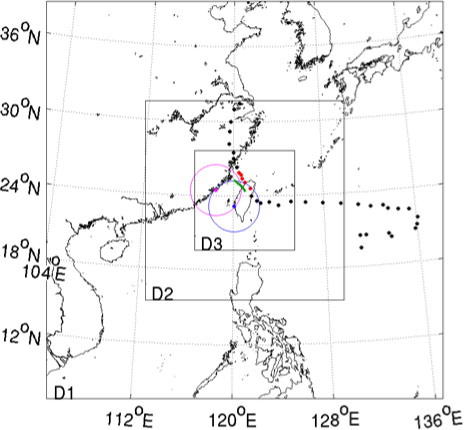
This study employs the Advanced Research WRF (ARW) model version 3.2.1 (Skamarock et al., 2008) with two-way interactive, triple-nested domains (Fig. 1). Domain 1 has 89×89 horizontal grid points with a 40.5-km spacing, domain 2 has 133×133 horizontal grid points with a 13.5-km spacing, and domain 3 has 199×199 horizontal grid points with a 4.5-km spacing. There are 28 vertical eta levels with a model top of 50 hPa. The physics schemes are the Purdue Lin scheme (Lin et al., 1983) for microphysics, Kain-Fritsch scheme (Kain, 2004) for cumulus parameterisation, Noah land-surface model (Chen and Dudhia, 2001) and Yonsei University (YSU) planetary boundary layer scheme (Hong et al., 2006). The prognostic variables contain the three-dimensional velocity components (u, v and w), perturbation potential temperature (θ′), perturbation geopotential (ϕ′), perturbation surface pressure of dry air (µ′) and mixing ratios of water vapour (q _v ), cloud water (q _c ), rain (q _r ), cloud ice (q _i ), snow (q _s ) and graupel (q _g ).

Fig. 1 The two-way interactive, triple-nested domains. The black and red dots mark the best track of Typhoon Morakot (2009) with a 6-hour interval provided by the Central Weather Bureau (CWB). The red dots correspond to the period (0000 UTC 8 to 0000 UTC 9 Aug) of the nature run, whose track is indicated by the green line. The blue dot and circle mark the location and maximum unambiguous range of the RCCG radar, and the magenta ones represent an imaginary radar at Kinmen.

A radar observation operator is implemented in our WRF-LETKF system for the simulation and assimilation of V _r and Z _h observations. This operator handles both spatial interpolation and variable conversion. For the spatial interpolation, the operator finds the nearest eight grid points (located in terrain-following coordinates) for each radar observation point (located in spherical coordinates) and then interpolates relevant model variables from the eight points to the observation point by inverse distance weighting. The surface curvature and atmospheric refraction of the Earth are considered with the 4/3 Earth radius model, and terrain blocking is also taken into account. Subsequently, the interpolated model variables are converted to V _r and Z _h through the relations in Sun and Crook (1997). V _r is computed by summing up the projections of u, v, w and terminal velocity v _t on the radar beam as6

where x, y and z are the Cartesian coordinates with the origin at the radar site, and v _t is calculated by assuming a Marshall-Palmer drop size distribution (DSD; Marshall and Palmer, 1948) as7

where p ₀ is the surface pressure, is the base-state pressure, and ρ _a is the air density. Z _h is calculated also by assuming a Marshall-Palmer DSD as8

It needs to be noticed that eq. (8) considers only the reflectivity contributed by rain. This is not a problem for the OSSEs, in which both the model and observation operator are assumed to be perfect; however, when real reflectivity observations are assimilated, it is necessary to examine whether eq. (8) is adequate or the reflectivity contributed by ice-phase hydrometeors has to be considered as well (e.g. Smith et al., 1975).

3. Experimental design

3.1. Nature run and simulated radar observations

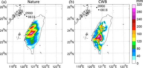
To evaluate a newly-established data assimilation system, OSSEs are often carried out with a simulated long run regarded as the nature run (truth), which can serve as a standard for quantitative comparison. To simulate a nature run that approximates to the period when Typhoon Morakot (2009) brought Taiwan the heaviest rainfall, we make 24-hour 40-member ensemble forecasts starting at 0000 UTC 8 Aug and then pick out the most realistic member. The initial and boundary conditions of each member are generated from the National Centers for Environmental Prediction (NCEP) 1°×1° Final Analysis (FNL) data and perturbed based on the background error covariances constructed for the WRF-3DVAR system. Compared with the Central Weather Bureau (CWB) observations (Fig. 2), the member chosen as the nature run has a similar track and 6-hour rainfall accumulation (1800 UTC 8 to 0000 UTC 9) despite a slight track deviation (Fig. 1) while the other members deviate more. During the 24 hours, the centre of Typhoon Morakot (2009) moved from northern Taiwan to northern Taiwan Strait. Meanwhile, the westerly flow that converged the moist southwest monsoon and typhoon circulation continuously impinged on central and southern Taiwan and resulted in long-lasting heavy rainfall on the windward slopes of the CMR, where a catastrophic landslide occurred as mentioned in the introduction.

Fig. 2 (a) The 700-hPa circulation centre (black dots) and 6-hour rainfall accumulation (colour shading) for the nature run and (b) the best track and 6-hour rainfall accumulation for the Central Weather Bureau (CWB) observations from 1800 UTC 8 to 0000 UTC 9 Aug.

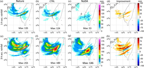
Figure 3a–d shows the field of w at an altitude of 1 km and the composite of the maximum q _r at all levels from 1800 to 2100 UTC for the nature run. The spiral rainbands characterised by strong updrafts and abundant rain are simulated, and they move from Taiwan Strait to the land along the westerly flow. For a closer look at their evolution, we mark the updraft locations (shaded by red and yellow) of individual rainbands by upper-case letters. At 1800 UTC, a rainband A with a cluster of weaker updrafts is in its formation stage while an elongated rainband B has already reached its maximum intensity. From 1800 to 2100 UTC, the updrafts in rainband A intensify and become aligned while rainband B gradually dissipates. A rainband C forms to the south of rainband B at 1900 UTC but does not intensify with time. The characteristics of these simulated rainbands are similar to the real ones observed in Liou et al. (2013), which found that inner (younger) rainbands intensified and moved southwards while outer (older) rainbands dissipated during this period of Typhoon Morakot (2009). As to non-rainband areas, updrafts and downdrafts mostly occur on the windward and lee slopes of the CMR, respectively. The former may induce local convective rainfall in addition to the rain advected from Taiwan Strait. Figure 4a and 4e show the 1- and 3-hour rainfall accumulations since 1800 UTC for the nature run. It can be seen that the spiral rainbands are responsible for the majority of the rainfall, and the orographic effect of the CMR on rainfall intensity and distribution is significant due to the contrast between the windward and lee slopes (e.g. Wu et al., 2002; Fang et al., 2011).

Fig. 3 The field of w (colour shading) at an altitude of 1 km and the composite of the maximum q _r at all levels (contours at 1 g kg⁻¹). Columns from left to right: 1800, 1900, 2000 and 2100 UTC 8 Aug. Rows from top to bottom: the nature run, CTRL and NoDA. The grey shading indicates the mountain areas higher than 1 km. The upper-case letters mark the spiral rainbands discussed in the text. The RCCG radar is situated in the centre (120.0860°E, 23.1467°N).

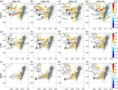
Fig. 4 The (a–c) 1-hour and (e–g) 3-hour rainfall accumulations since 1800 UTC 8 Aug for the nature run, CTRL and NoDA and (d and h) the improvement, which is computed by subtracting the absolute error in CTRL from that in NoDA. The RCCG radar is situated in the centre (120.0860°E, 23.1467°N).

The RCCG radar chosen for this OSSE study is situated at the southwestern coast of Taiwan (120.0860°E, 23.1467°N; Fig. 1), belonging to CWB's S-band Doppler weather radar network. The V _r and Z _h observations of RCCG are simulated according to the nature run and assimilated in this study because its radar coverage overlaps main rainfall areas. This radar is designed to have a maximum unambiguous range of 230 km, a volume scan period of 7.5 minutes and nine plan position indicator (PPI) elevation angles ranging from 0.5° to 19.5°. For weather radars including RCCG, the range gate spacing depends on the pulse repetition frequency and ranges from dozens to hundreds of meters. Such spatial resolution is usually one order higher than the horizontal grid resolution used in regional NWP. To save computational cost and avoid the error dependence between adjacent range-gate observations (e.g. Berenguer and Zawadzki, 2008), the spatial resolution of radar data needs to be lowered to the level of the grid resolution as a pre-process of data assimilation. There are two popular approaches: data thinning (e.g. Chung et al., 2009; Montmerle and Faccani, 2009) and superobbing (e.g. Lindskog et al., 2004; Zhang et al., 2009; Kawabata et al., 2011; Weng and Zhang, 2012). The former selects certain range gates with proper intervals and discards the others; the advantage is that extreme values, including maxima and minima, may be preserved instead of being smoothed out so that the magnitude of convective-scale features could be better represented. The latter produces superobservations (SOs), each of which is the weighted average of neighbouring range gates; the advantage is that SOs express the lower-resolution information with smaller representative errors. Since data selection is not the focus in the OSSEs, we bypass both approaches but directly simulate lower-resolution observations with the observation operator. The radial and azimuth spacings are 5 km and 5°, respectively. The observations are available only in the areas where Z _h >0 dBZ, and the errors are 3 m s⁻¹ for V _r and 5 dBZ for Z _h . In addition to RCCG, an imaginary radar is situated at Kinmen (118.4181°E, 24.4615°N; Fig. 1) for a sensitivity experiment of increasing the observations in the upstream area of the westerly flow.

3.2. Assimilation experiments

Figure 5 shows the schematic design of the OSSEs, in which CTRL stands for a control assimilation experiment and NoDA stands for the experiment without radar data assimilation. Both experiments use the same 40-member initial ensemble, which is initialised 12 hours later (1200 UTC) than the initialisation of the nature run to obtain a different synoptic-scale condition that helps alleviate the identical-twin problem in perfect-model experiments (Arnold and Dey, 1986). Again, this ensemble is generated from the FNL data and perturbed with WRF-3DVAR. For CTRL and NoDA, we assume the FNL data inherently contain the synoptic-scale information from assimilating conventional and satellite observations and discuss only the impact from adding radar data assimilation. The initial ensemble is perturbed at domain 1 based on synoptic-scale background error statistics and hence integrated for a few hours to spin up the convective-scale background error structure at domain 3. Subsequently, CTRL assimilates the simulated RCCG observations from 1600 to 1800 UTC while NoDA does not. Please note that, in CTRL, the prognostic variables are analysed only at domain 3 because all the observations are located in the innermost domain and domains 1 and 2 can share analysis information via the two-way interaction. Finally, the analysis mean in CTRL and the forecast mean in NoDA at 1800 UTC separately initialise 6-hour deterministic nowcasts for quantitative comparison. Furthermore, the assimilation strategies in CTRL include the assimilation of both V _r and Z _h observations, a 2-hour assimilation period, a 15-minute analysis cycle interval and a 12-km horizontal covariance localisation radius for all the prognostic variables. To probe into the sensitivity to each of these strategies, we also carry out a series of assimilation experiments in addition to CTRL, listed in Table 1.

Fig. 5 The schematic design of the OSSEs. The black dots represent the simulated observations of the RCCG radar. The single and triple arrows represent single and ensemble simulations, respectively.

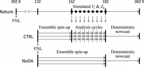
Table 1. The list of the assimilation experiments

Assimilation strategies
Name	Assimilated observations	Length of the assimilation period	Analysis cycle interval	Horizontal covariance localisation radius
CTRL	V r , Z h (RCCG)	2 hours	15 minutes	12 km (all variables)
VR	V r (RCCG)	*	*	*
ZH	Z h (RCCG)	*	*	*
VZ0	V r , Z h , 0-dBZ Z h (RCCG)	*	*	*
KM	V r , Z h (RCCG, Kinmen)	*	*	*
P1	*	1 hour	*	*
P3	*	3 hours	*	*
I7.5	*	*	7.5 minutes	*
I30	*	*	30 minutes	*
UV24	*	*	*	24 km (u, v), 12 km (others)
UV36	*	*	*	36 km (u, v), 12 km (others)
NoDA	No data assimilation

*denotes the same setting as CTRL.

4. Results

4.1. Analysis performance

In our experiments, the ensemble is spun up prior to the analysis cycles. This is essential for establishing a reasonable convective-scale background error structure. Figure 6 shows the ensemble mean errors and ensemble spreads of u, v, w, θ′, q _v , q _c and q _r from 1200 to 1800 UTC for NoDA. A reasonable ensemble spread is supposed to approach the ensemble mean error (Murphy, 1988). The statistics shown in Fig. 6 are computed by performing a root-mean-square operation on the grid points located at the lowest 14 levels and within RCCG's maximum unambiguous range. This cylindrical statistical area is chosen because it encloses all the simulated observations and therefore approximates to the area where data assimilation takes effect. It can be seen that the mean errors and spreads of all the variables change quickly in the first 4 hours and then stabilise at similar levels, with differences smaller than 10% (except u). This indicates that the ensemble has not been appropriately spun up to represent the convective-scale background error structure until 1600 UTC. Hence, 1600 UTC is the start time of the analysis cycles in CTRL. The exception in u tells that the ensemble mean has an excessive deviation of u compared with the nature run. This deviation is inherited from the FNL data at different initialisation time.

Fig. 6 The ensemble mean errors (solid) and ensemble spreads (dashed) of (a) u, (b) v, (c) w, (d) θ′, (e) q _v , (f) q _c and (g) q _r from 1200 to 1800 UTC 8 Aug for NoDA, computed by performing a root-mean-square operation on the grid points located at the lowest 14 levels and within RCCG's maximum unambiguous range.

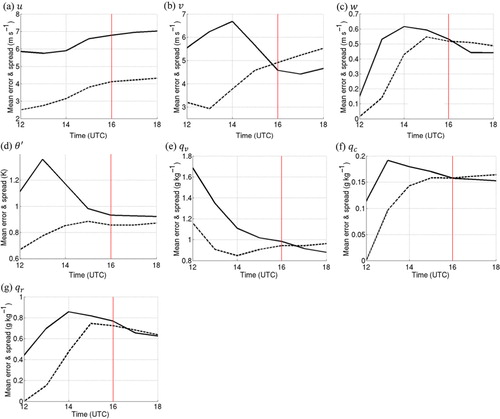
Figure 7 zooms the time interval of Fig. 6 into 1600–1800 UTC and includes the mean errors and spreads from CTRL. The sawtooth-like curves represent the alternate forecast and analysis steps in CTRL. Obviously, u, v, w and q _r are the most improved prognostic variables during the assimilation period. Their mean errors reach the minima of 4.5 m s⁻¹, 3.3 m s⁻¹, 0.35 m s⁻¹ and 0.34 g kg⁻¹ at the final analysis step, which are 36, 29, 21 and 45% lower than those in NoDA, respectively (Fig. 7a–c and 7g; also see Table 2). The outstanding analysis performance of u, v, w and q _r is reasonable because these variables are directly related to the observation variables as in eqs. (6–8). However, w has the least improvement among the four. This can be attributed to the fact that, as the magnitude of w is one-order smaller than those of u and v, the projection of w on the radar beam at low elevation angles is negligible and even smaller than the observation error of V _r ; that is, w is almost unobserved. For the other variables (θ′, ϕ′, µ′, q _v , q _c , q _i , q _s and q _g ) which are completely unobserved, their analysis accuracies depend on the reliability of the ensemble-based error covariances between these variables and the observations. This reliability looks robust for q _c because its mean error is reduced at every analysis step (Fig. 7f). As to θ′ and q _v , their mean errors do not change much at analysis steps but decrease at forecast steps instead (Fig. 7d and 7e) for being dynamically adjusted by other improved variables. In general, the mean errors and spreads become more consistent after radar data assimilation for most of the prognostic variables. The results of ϕ′, μ′, q _i , q _s and q _g are not shown because no significant differences are found with them between CTRL and NoDA.

Fig. 7 As in Fig. 6, but the time interval is zoomed into 1600–1800 UTC (after the red line in Fig. 6). The ensemble mean errors (red solid) and ensemble spreads (red dashed) from CTRL are included.

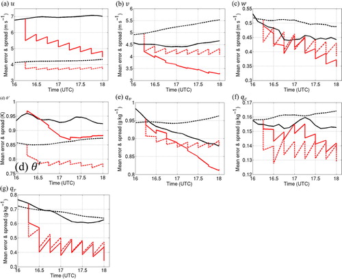
Table 2. The final analysis mean errors of u, v, w, θ′, q _v , q _c and q _r at 1800 UTC 8 Aug for all the assimilation experiments, computed by performing a root-mean-square operation on the grid points located at the lowest 14 levels and within RCCG's maximum unambiguous range, and their improvement percentages compared with NoDA

Mean errors and the improvement percentages compared with NoDA
Name	u (m s^−1)	%	v (m s^−1)	%	w (m s^−1)	%	θ′ (K)	%	q v (g kg^−1)	%	q c (g kg^−1)	%	q r (g kg^−1)	%
CTRL	4.5	36	3.3	29	0.35	21	0.88	4	0.81	7	0.14	11	0.34	45
VR	4.9	30	4.1	13	0.41	7	4	Co-action 7	0.87	1	0.14	6	0.57	8
ZH	6.3	11	3.8	19	0.39	12	0.97	--5	0.87	1	0.14	7	0.38	39
VZ0	4.5	35	Co-action 3.2	Co-action 31	Co-action 0.33	Co-action 26	Co-action 0.87	Co-action 6	0.82	7	Co-action 0.13	Co-action 13	Co-action 0.31	Co-action 51
KM	Co-action 3.6	Co-action 49	Co-action 2.7	Co-action 42	Co-action 0.31	Co-action 31	Co-action 0.84	Co-action 9	Co-action 0.78	Co-action 11	Co-action 0.12	Co-action 19	Co-action 0.27	Co-action 57
P1	5.1	27	3.9	17	0.37	17	Co-action 0.87	Co-action 6	0.86	2	0.14	8	0.37	41
P3	Co-action 4.2	Co-action 40	Co-action 3.2	Co-action 32	Co-action 0.34	Co-action 23	Co-action 0.86	Co-action 7	Co-action 0.80	Co-action 9	Co-action 0.13	Co-action 12	Co-action 0.33	Co-action 47
I7.5	Co-action 4.2	Co-action 40	Co-action 3.2	Co-action 30	Co-action 0.32	Co-action 27	0.92	0	0.87	1	0.14	11	Co-action 0.30	Co-action 52
I30	5.0	29	3.8	19	0.38	14	Co-action 0.88	Co-action 5	0.84	4	0.14	7	0.43	32
UV24	Co-action 4.1	Co-action 42	Co-action 3.2	Co-action 31	Co-action 0.34	Co-action 23	0.89	4	0.82	6	0.14	10	Co-action 0.34	Co-action 46
UV36	Co-action 4.0	Co-action 43	3.4	27	Co-action 0.35	Co-action 22	0.89	3	0.85	3	0.14	9	0.37	41
NoDA	7.0	4.7	0.44	0.92	0.88	0.15	0.63

The frames are used to highlight better performance than CTRL.

To understand the spatial distribution of the analysis performance, the field of w at an altitude of 1 km and the composite of the maximum q _r at all levels for the analysis mean in CTRL (Fig. 3e) and forecast mean in NoDA (Fig. 3i) are compared with the nature run (Fig. 3a) at 1800 UTC. The structure of spiral rainbands is clearly established in CTRL but rather weak in NoDA after the ensemble is averaged to obtain the mean state. This reflects a fact that the convection patterns of different members can become much alike after radar observations are assimilated. The fields of w and q _r in CTRL accurately correspond with those in the nature run, especially for the area close to RCCG (centre of the map) such as rainband B. By contrast, the high-q _r areas in NoDA are incorrectly located and short of strong updrafts. Although rainband A is not perfectly represented in the CTRL analysis, it is still far better than that in NoDA. There are two reasons for the relatively inaccurate analysis of rainband A. First, the radar observations in this area are sparse and only available at high levels. Second, during the assimilation period, the unobserved inflow from the north of this area continuously dilutes the updated information obtained at the analysis time. It is foreseeable that the improvement of prognostic variables will fade away with the forecast time as more and more unobserved convective systems move into the statistical area after the assimilation period, and therefore increasing the observations in the upstream area of the westerly flow is considered an effective way to lengthen the positive impact of radar data assimilation, which is verified later.

4.2. QPN performance

The information of weather forecasting can be delivered either deterministically or stochastically. The former forecasts a unique atmospheric state by a single model simulation, and the latter forecasts the probability distribution of the state by an ensemble of model simulations. However, we should note that the ensemble mean is not a good estimate for precipitation because peak values are smoothed out for the dislocation of precipitation areas between different members. Instead, more sophisticated statistical methods (e.g. Wilks, 1990; Krzysztofowicz et al., 1993; Ruiz et al., 2009) can be implemented for probabilistic quantitative precipitation forecasting (PQPF). For simplicity, this study carries out the previously-mentioned 6-hour deterministic nowcasts, whose QPN skill is evaluated by means of four different criteria: the root-mean-square error (RMSE), the spatial correlation coefficient (SCC), the equitable threat score (ETS) and the bias score (Bias) compared with the nature run. The former two are used to quantify the overall QPN performance while the latter two focus on the performance for heavy rainfall, which is defined with an hourly rainfall threshold of 15 mm in this study. The 15-mm threshold is also the criterion for CWB to issue a heavy rain advisory. Figure 8 shows the RMSE, SCC, ETS and Bias of the predicted hourly rainfall from 1800 UTC 8 to 0000 UTC 9 Aug for CTRL and NoDA, computed within RCCG's maximum unambiguous range. Obviously, CTRL has a lower RMSE, a higher SCC, a higher ETS and a Bias closer to 1, all of which mean a better prediction than NoDA at each of the 6 hours. At the first hour, the RMSE reaches a minimum of 7.4 mm, which is a 39% improvement (also see Table 3), and the SCC has an outstanding value of 0.83. During the following hours, the improvement gradually decreases and the evolution trends of the four standards are similar between CTRL and NoDA; the same phenomenon also exists in the nowcasts of prognostic variables (not shown). This indicates that the single-radar data assimilation in this OSSE setup can substantially correct the model state within the limited radar coverage but cannot alter the evolution trend driven by synoptic-scale conditions.

Fig. 8 The (a) RMSE, (b) SCC, (c) ETS and (d) Bias of the predicted hourly rainfall compared with the nature run from 1800 UTC 8 to 0000 UTC 9 Aug for CTRL (red) and NoDA (black), computed within RCCG's maximum unambiguous range. The hourly rainfall threshold of the ETS and Bias is 15 mm.

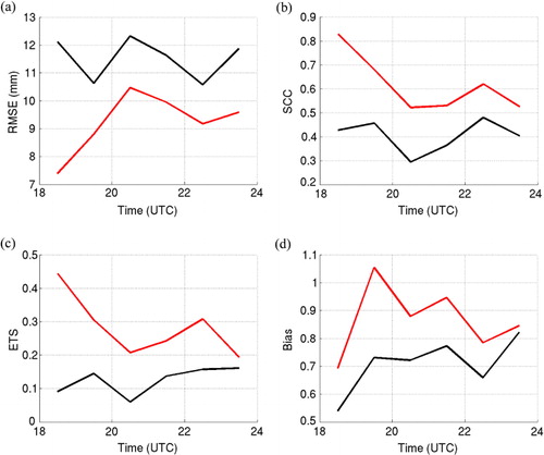
Table 3. The RMSEs of the predicted 1-, 2-, 3-, 4-, 5- and 6-hour rainfall accumulations since 1800 UTC 8 Aug for all the assimilation experiments, computed within RCCG's maximum unambiguous range, and their improvement percentages compared with NoDA

RMSEs and the improvement percentages compared with NoDA
Name	1-hour rain (mm)	%	2-hour rain (mm)	%	3-hour rain (mm)	%	4-hour rain (mm)	%	5-hour rain (mm)	%	6-hour rain (mm)	%
CTRL	7.4	39	12.5	38	16.7	39	22.0	35	26.8	31	30.6	32
VR	11.5	5	17.3	14	22.6	17	27.5	19	31.8	19	36.5	19
ZH	8.2	32	14.2	29	20.1	27	25.9	23	31.5	19	36.8	18
VZ0	Co-action 6.7	Co-action 44	12.6	37	17.8	35	22.8	32	27.8	29	31.9	29
KM	Co-action 6.2	Co-action 49	Co-action 11.1	Co-action 45	Co-action 15.6	Co-action 43	Co-action 18.5	Co-action 45	Co-action 21.9	Co-action 44	Co-action 26.8	Co-action 40
P1	9.0	26	14.3	29	18.4	33	23.0	32	27.9	28	33.1	26
P3	Co-action 7.2	Co-action 41	13.0	35	17.2	37	22.2	34	Co-action 26.5	Co-action 32	Co-action 30.3	Co-action 32
I7.5	Co-action 6.9	Co-action 43	Co-action 12.0	Co-action 40	16.7	39	22.3	34	27.7	29	31.2	30
I30	8.5	29	14.1	30	17.8	35	23.1	32	28.1	28	32.3	28
UV24	Co-action 7.0	Co-action 42	Co-action 12.2	Co-action 39	16.9	38	22.5	33	27.7	29	31.0	31
UV36	Co-action 7.2	Co-action 40	Co-action 12.1	Co-action 40	17.0	38	22.6	33	27.3	30	31.5	30
NoDA	12.1	20.1	27.4	33.7	39.0	44.8

The frames are used to highlight better performance than CTRL. RMSEs=root-mean-square errors.

It has been mentioned in Section 3 that the spiral rainbands are responsible for the majority of the typhoon-induced rainfall. To examine whether the tracked rainbands A, B and C in the nature run are well predicted, we also mark the updraft locations of individual rainbands in the forecast maps of w and q _r for CTRL (Fig. 3f–h) and NoDA (Fig. 3j–l) by upper-case letters. The same letters are used if the locations match those in the nature run. It can be seen that rainbands A and B correctly remain at 1900 UTC in CTRL but never appear in NoDA. However, in both CTRL and NoDA, the rainband C which should form at 1900 UTC is always missing while a false rainband D occurs instead. At 2000 UTC, the rainbands A and B in CTRL still remain but have inaccurate intensities. At 2100 UTC, rainband B dissipates just like the way in the nature run but rainband A fails in intensification. The evolution of these four rainbands reveals the effect of radar data assimilation. Rainbands A and B can be well predicted because of their presence at the final analysis, and the prediction of rainband B surpasses that of rainband A for assimilating denser observations close to RCCG. Rainbands C and D respectively represent a miss and a false alarm, which may result from the incorrect information of atmospheric stability conditions and convergence zones in their nearby areas, where no radar data are assimilated.

Figure 4 shows the 1- and 3-hour rainfall accumulations since 1800 UTC for the nature run, CTRL and NoDA and the improvement, which is computed by subtracting the absolute error in CTRL from that in NoDA. The largest 1-hour rainfall accumulation, which occurs in the area of rainband B, is better predicted in CTRL than in NoDA (Fig. 4a–c). The maximum in CTRL (124 mm) is close to that in the nature run (135 mm) while the maximum in NoDA (53 mm) is seriously underforecasted and incorrectly located. These remarkable improvements can be potential benefits to early warning systems, which demand accurate rainfall distribution and intensity in short terms. The improvement map shows that not only the areas of spiral rainbands but also the other areas within RCCG's coverage can benefit from radar data assimilation (Fig. 4d). As to the 3-hour rainfall accumulation, the false rainband D predicted in both CTRL and NoDA leads to a southward deviation of the heaviest rainfall area (Fig. 4e–g); nevertheless, the peak rainfall intensity is still better forecasted in CTRL and the improvement is also widespread (Fig. 4h).

4.3. Sensitivities to individual assimilation strategies

Based on the analysis and QPN performances in CTRL, the sensitivities of these performances to individual assimilation strategies are investigated. For an overview of the results, the final analysis mean errors of u, v, w, θ′, q _v , q _c and q _r are listed in Table 2 and the RMSEs of the predicted 1- to 6-hour rainfall accumulations are listed in Table 3 for all the below-mentioned sensitivity experiments, as well as their improvement percentages compared with NoDA. In both tables, the improvement percentage is highlighted with a frame if it is larger than that in CTRL. First, we examine the impact of assimilating only one observation variable, either V _r (experiment VR) or Z _h (experiment ZH). In Table 2, it can be seen that CTRL outperforms both VR and ZH for almost all the prognostic variables. In the comparison between VR and ZH, the variables with error differences larger than 10% are u, θ′ and q _r , in which u and θ′ are better in VR while q _r is better in ZH. These results are reasonable because of the relations in the observation operator. In Table 3, ZH has more accurate 1- to 4-hour rainfall accumulations but a less accurate 6-hour rainfall accumulation than VR. This infers that the QPN performance responds to the adjustment of hydrometeors more quickly than the adjustment of winds. Again, CTRL outperforms both VR and ZH for all different rainfall accumulation durations and confirms the importance of coupling the adjustments of winds and hydrometeors.

Second, the assimilation of 0-dBZ Z _h assumed in the echo-free zone (EFZ) was proven helpful to the suppression of spurious convective cells (e.g. Tong and Xue, 2005; Kawabata et al., 2011), and we are interested in whether this approach also benefits the precipitation nowcast for this typhoon case. In experiment VZ0, the reflectivity in the EFZ is set to be 0 dBZ and assimilated along with the existing V _r and Z _h observations. Compared with CTRL, VZ0 has more accurate analyses of v, w, θ′, q _c and q _r (Table 2) and the additional information is most influential during the 1-hour precipitation nowcast (Table 3). Figure 9a also shows that the improvement areas exceed the degradation areas for the predicted 1-hour rainfall accumulation. However, the improvement quickly vanishes beyond 1 hour, and the computational cost for VZ0 is about 50% larger than that for CTRL at analysis steps due to extra observations. This implies that the employment of assimilating 0-dBZ Z _h depends on whether the limited improvement is considered worthy of the increased computational cost. Considering that our experiments are carried out under a perfect model assumption, this approach may be helpful in real cases if the NWP model has a systematic error (e.g. a wet bias).

Fig. 9 The improvement of the predicted 1-hour rainfall accumulation since 1800 UTC 8 Aug for VZ0, KM and UV24 compared with CTRL. The RCCG radar is situated in the centre (120.0860°E, 23.1467°N), and the imaginary Kinmen radar is situated at the northwest corner (118.4181°E, 24.4615°N).

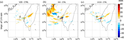
Third, we have expected previously that increasing the observations in the upstream area of the westerly flow can lengthen the positive impact of radar data assimilation. Thus, experiment KM is carried out to assimilate the V _r and Z _h observations of an imaginary radar at Kinmen in addition to those of RCCG. As expected, the results of KM are unrivalled in all aspects among all the assimilation experiments (Table and 3 ). Figure 9b also shows that the improvement of the predicted 1-hour rainfall accumulation for KM compared with CTRL is widespread and significant, especially near the Kinmen radar. As expected, the observation coverage over the areas of convective initiation is the most dominant factor of the analysis and QPN performances.

Fourth, given a fixed observation coverage, further improvement is still possible by modifying the length of the assimilation period and the analysis cycle interval. In experiments P1 and P3, the assimilation period is shortened to 1 hour and lengthened to 3 hours, respectively. As a result, P3 has smaller final analysis mean errors for all the prognostic variables than those in CTRL while P1 has larger errors instead (Table 2). P3 also improves the 1-, 5- and 6-hour rainfall accumulations compared with CTRL (Table 3). This suggests that an assimilation period long enough to accumulate observation information is beneficial for QPN. In experiments I7.5 and I30, the analysis cycle interval is shortened to 7.5 minutes and lengthened to 30 minutes, respectively. These intervals are the multiples of RCCG's volume scan period. Likewise, the performances are enhanced in I7.5 but worsened in I30 (Table and 3 ). Frequently injecting observation information can further improve the 1- and 2-hour rainfall accumulations. In conclusion, increasing the length of the assimilation period and assimilating every 7.5-minute volume scan of the operational radar data can be regarded as the proper strategy to optimise the QPN skill, but once again the user needs to decide whether the limited improvement is worthy of the largely-increased computational cost due to extra analysis cycles.

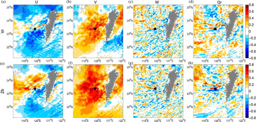
Last, to illustrate the reason to propose the mixed localisation method in this study, the background error correlations at 1800 UTC for CTRL between the fields of the prognostic variables (u, v, w and q _r ) and the observation variables (V _r and Z _h ) at a point in the area of rainband B are plotted in Fig. 10. It is obvious that the patterns of the correlations reveal a flow-dependent rainband structure near this point, and these horizontal correlations are less noisy for u and v than the others; that is, the horizontal wind field that has a larger scale than embedded convective cells dominates the typhoon circulation. This leads to a straightforward idea of extending the horizontal covariance localisation radius for u and v. With an optimal radius of 12 km for the other prognostic variables, 12, 24 and 36 km are used as the radius for u and v in experiments CTRL, UV24 and UV36, respectively. Compared with CTRL, UV24 has more accurate analyses of u, v, w and q _r and UV36 has better u and w (Table 2). This indicates that the variables directly related to V _r and Z _h benefit from suitable mixed localisation in this typhoon case. From Table 3, UV24 and UV36 also provide more accurate 1- and 2-hour rainfall accumulations than CTRL. Moreover, Fig. 9c shows a signature that the most improved area corresponds with the area of the densely-observed rainband B although some slight degradation also appears.

Fig. 10 The background error correlations at 1800 UTC for CTRL, between the fields of the prognostic variables (u, v, w and q _r from left to right) at an altitude of 1 km and the observation variables (V _r and Z _h from top to bottom) at a point (black dot) in the area of rainband B. The coordinates of the point are 119.8138°E, 23.3372°N, 1 km. The grey shading indicates the mountain areas higher than 1 km. The RCCG radar is situated in the centre (120.0860°E, 23.1467°N).

5. Summary and future prospects

A WRF-LETKF Doppler radar data assimilation system is developed in this study, and its QPN skill for the period that Typhoon Morakot (2009) brought Taiwan the heaviest rainfall is evaluated with a series of OSSEs. A 24-hour simulation that has the most realistic track and rainfall is taken as the nature run, and the V _r and Z _h observations of CWB's RCCG radar are simulated and assimilated to improve the analysis and QPN performances. Even with the OSSE framework, this study shows that achieving accurate QPN with radar observations is not trivial. The main conclusions of this study are summarised as follows:

1. The horizontal winds and rain mixing ratio are the most improved prognostic variables after the assimilation period because of their direct relations to the observation variables, and the patterns of spiral rainbands become more consistent between different ensemble members after radar data assimilation, especially for the areas close to RCCG.

2. The improvement of the predicted rainfall intensity and distribution is available for the entire 6-hour deterministic nowcast, no matter within the full radar coverage or only the heavy rainfall areas. However, this improvement fades away with the forecast time and both the nowcasts with and without radar data assimilation have similar evolution trends driven by synoptic-scale conditions. The evolution of the spiral rainband can be better predicted if the rainband is captured in the final analysis. The forecasted peak rainfall intensity is also remarkably improved, which is important to disaster early warning systems.

3. A series of sensitivity experiments are carried out to develop proper assimilation strategies for this case. As a result, the QPN performance responds to the assimilation of Z _h more quickly than the assimilation of V _r while assimilating both is most recommended. The observation coverage over the areas of convective initiation is found to be the most dominant factor of the analysis and QPN performances. Adding the assimilation of 0-dBZ Z _h , lengthening the assimilation period and assimilating every 7.5-minute volume scan of the operational radar data also yield better QPN performances, especially for the first hour, despite the large increase of computational cost. Furthermore, a mixed localisation method is proposed and found to improve the variables directly related to V _r and Z _h as well as the precipitation nowcast within 2 hours when the horizontal covariance localisation radius for horizontal winds is suitably extended.

Based on the conclusions of this OSSE study, we are currently engaging our system in assimilating real radar data. More different model configurations (resolutions, physics, initial and boundary conditions, etc.), assimilation strategies and radar numbers will be tested for the optimisation of the QPN skill. In addition to deterministic QPN, PQPFs will also be made to extract useful uncertainty information from ensemble forecasts. Up to the present, some preliminary real-case results have shown the positive impact on QPN with our system and with the mixed localisation method, to be documented in future studies.

6. Acknowledgements

The authors are thankful for the valuable comments from the peer reviewers and suggestions provided by Prof. Eugenia Kalnay from the University of Maryland, Dr. Chris Snyder and Dr. Juanzhen Sun from the National Center for Atmospheric Research, Prof. Ming Xue from the University of Oklahoma, Prof. Fuqing Zhang from the Pennsylvania State University, Dr. Kao-Shen Chung from Environment Canada and Dr. Takemasa Miyoshi from the Institute of Physical and Chemical Research, Japan. This research is sponsored by Taiwan National Science Council, under Grants NSC-100-2625-M-008-002, NSC-101-2625-M-008-003 and NSC-101-2111-M-008-020, and Taiwan Typhoon and Flood Research Institute.

Notes

¹For real radar data, the lower limit of Z _h depends on the sensitivity of the radar and the criteria of quality control.

²With 8-cpu parallel computing, the wall-clock time needed to advance one 15-minute analysis cycle for CTRL is approximately 85 minutes (including 70 minutes for one forecast step of the 40-member ensemble and 15 minutes for one LETKF analysis step).

References

- Aksoy A. , Dowell D. C. , Snyder C . A multicase comparative assessment of the ensemble Kalman filter for assimilation of radar observations. Part II: short-range ensemble forecasts. Mon. Weather Rev. 2010; 138: 1273–1292.
- Anderson J. L . An ensemble adjustment Kalman filter for data assimilation. Mon. Weather Rev. 2001; 129: 2884–2903.
- Arnold C. P. Jr. , Dey C. H . Observing-systems simulation experiments: past, present, and future. Bull. Am. Meteorol. Soc. 1986; 67: 687–695.
- Berenguer M. , Zawadzki I . A study of the error covariance matrix of radar rainfall estimates in stratiform rain. Weather Forecast. 2008; 23: 1085–1101.
- Bishop C. H. , Etherton B. J. , Majumdar S. J . Adaptive sampling with the ensemble transform Kalman filter. Part I: theoretical aspects. Mon. Weather Rev. 2001; 129: 420–436.
- Browning K. A. , Collier C. G. , Larke P. R. , Menmuir P. , Monk G. A. , co-authors . On the forecasting of frontal rain using a weather radar network. Mon. Weather Rev. 1982; 110: 534–552.
- Caine N . The rainfall intensity-duration control of shallow landslides and debris flows. Geogr. Ann. 1980; 62A: 23–27.
- Caya A. , Sun J. , Snyder C . A comparison between the 4DVAR and the ensemble Kalman filter techniques for radar data assimilation. Mon. Weather Rev. 2005; 133: 3081–3094.
- Chen F. , Dudhia J . Coupling an advanced land surface-hydrology model with the Penn State-NCAR MM5 modeling system. Part I: model implementation and sensitivity. Mon. Weather. Rev. 2001; 129: 569–585.
- Chung K.-S. , Zawadzki I. , Yau M. K. , Fillion L . Short-term forecasting of a midlatitude convective storm by the assimilation of single–Doppler radar observations. Mon. Weather Rev. 2009; 137: 4115–4135.
- Evensen G . Sequential data assimilation with a nonlinear quasi-geostrophic model using Monte Carlo methods to forecast error statistics. J. Geophys. Res. 1994; 99: 10143–10162.
- Fang X. , Kuo Y.-H. , Wang A . The impacts of Taiwan topography on the predictability of Typhoon Morakot's record-breaking rainfall: a high-resolution ensemble simulation. Weather Forecast. 2011; 26: 613–633.
- Germann U. , Zawadzki I . Scale-dependence of the predictability of precipitation from continental radar images. Part I: description of the methodology. Mon. Weather Rev. 2002; 130: 2859–2873.
- Greybush S. J. , Kalnay E. , Miyoshi T. , Ide K. , Hunt B. R . Balance and ensemble Kalman filter localization techniques. Mon. Weather Rev. 2011; 139: 511–522.
- Guzzetti F. , Peruccacci S. , Rossi M. , Stark C. P . The rainfall intensity-duration control of shallow landslides and debris flows: an update. Landslides. 2008; 5: 3–17.
- Hamill T. M. , Snyder C . A hybrid ensemble Kalman filter-3D variational analysis scheme. Mon. Weather Rev. 2000; 128: 2905–2919.
- Hong S.-Y. , Noh Y. , Dudhia J . A new vertical diffusion package with an explicit treatment of entrainment processes. Mon. Weather Rev. 2006; 134: 2318–2341.
- Hunt B. R. , Kostelich E. J. , Szunyogh I . Efficient data assimilation for spatiotemporal chaos: a local ensemble transform Kalman filter. Physica D. 2007; 230: 112–126.
- Kain J. S . The Kain-Fritsch convective parameterization: an update. J. Appl. Meteorol. 2004; 43: 170–181.
- Kalnay E . Atmospheric Modeling, Data Assimilation and Predictability. 2003; New York, NY, USA: Cambridge University Press. 340.
- Kang J.-S. , Kalnay E. , Liu J. , Fung I. , Miyoshi T. , co-authors . “Variable localization” in an ensemble Kalman filter: application to the carbon cycle data assimilation. J. Geophys. Res. 2011; 116: D09110.
- Kawabata T. , Kuroda T. , Seko H. , Saito K . A cloud-resolving 4DVAR assimilation experiment for a local heavy rainfall event in the Tokyo metropolitan area. Mon. Weather Rev. 2011; 139: 1911–1931.
- Krzysztofowicz R. , Drzal W. J. , Drake T. R. , Weyman J. C. , Giordano L. A . Probabilistic quantitative precipitation forecasts for river basins. Weather Forecast. 1993; 8: 424–439.
- Le Dimet F.-X. , Talagrand O . Variational algorithms for analysis and assimilation of meteorological observations: theoretical aspects. Tellus A. 1986; 38: 97–110.
- Lin Y.-L. , Farley R. D. , Orville H. D . Bulk parameterization of the snow field in a cloud model. J. Clim. Appl. Meteorol. 1983; 22: 1065–1092.
- Lindskog M. , Salonen K. , Järvinen H. , Michelson D. B . Doppler radar wind data assimilation with HIRLAM 3DVAR. Mon. Weather Rev. 2004; 132: 1081–1092.
- Liou Y.-C. , Chen Wang T.-C. , Tsai Y.-C. , Tang Y.-S. , Lin P.-L. , co-authors . Structure of precipitating systems over Taiwan's complex terrain during Typhoon Morakot (2009) as revealed by weather radar and rain gauge observations. J. Hydrology. 2013; 506: 14–25.
- Mandapaka P. V. , Germann U. , Panziera L. , Hering A . Can Lagrangian extrapolation of radar fields be used for precipitation nowcasting over complex Alpine orography?. Weather Forecast. 2012; 27: 28–49.
- Marshall J. S. , Palmer W. McK . The distribution of raindrops with size. J. Meteorol. 1948; 5: 165–166.
- Miyoshi T. , Sato Y. , Kadowaki T . Ensemble Kalman filter and 4D-Var intercomparison with the Japanese operational global analysis and prediction system. Mon. Weather Rev. 2010; 138: 2846–2866.
- Montmerle T. , Faccani C . Mesoscale assimilation of radial velocities from Doppler radars in a preoperational framework. Mon. Weather Rev. 2009; 137: 1939–1953.
- Murphy J. M . The impact of ensemble forecasts on predictability. Q. J. Roy. Meteorol. Soc. 1988; 114: 463–493.
- NCDR. Disaster Survey and Analysis of Morakot Typhoon (in Chinese) . 2010; New Taipei City, Taiwan: National Science and Technology Center for Disaster Reduction. 109.
- Ott E. , Hunt B. R. , Szunyogh I. , Zimin A. V. , Kostelich E. J. , co-authors . A local ensemble Kalman filter for atmospheric data assimilation. Tellus A. 2004; 56: 415–428.
- Ruiz J. , Saulo C. , Kalnay E . Comparison of methods used to generate probabilistic quantitative precipitation forecasts over South America. Weather Forecast. 2009; 24: 319–336.
- Sasaki Y . An objective analysis based on the variational method. J. Meteorol. Soc. Jpn. 1958; 36: 77–88.
- Skamarock W. C. , Klemp J. B. , Dudhia J. , Gill D. O. , Barker D. M. , co-authors . A Description of the Advanced Research WRF Version 3. 2008; Boulder, CO, USA: National Center for Atmospheric Research. 113.
- Smith P. L. Jr. , Myers C. G. , Orville H. D . Radar reflectivity factor calculations in numerical cloud models using bulk parameterization of precipitation processes. J. Appl. Meteorol. 1975; 14: 1156–1165.
- Snook N. , Xue M. , Jung Y . Ensemble probabilistic forecasts of a tornadic mesoscale convective system from ensemble Kalman filter analyses using WSR-88D and CASA radar data. Mon. Weather Rev. 2012; 140: 2126–2146.
- Sugimoto S. , Crook N. A. , Sun J. , Xiao Q. , Barker D. M . An examination of WRF 3DVAR radar data assimilation on its capability in retrieving unobserved variables and forecasting precipitation through observing system simulation experiments. Mon. Weather Rev. 2009; 137: 4011–4029.
- Sun J . Initialization and numerical forecasting of a supercell storm observed during STEPS. Mon. Weather Rev. 2005; 133: 793–813.
- Sun J. , Crook N. A . Dynamical and microphysical retrieval from Doppler radar observations using a cloud model and its adjoint. Part I: model development and simulated data experiments. J. Atmos. Sci. 1997; 54: 1642–1661.
- Sun J. , Xue M. , Wilson J. W. , Zawadzki I. , Ballard S. P. , co-authors . Use of NWP for nowcasting convective precipitation: recent progress and challenges (early online release). Bull. Am. Meteorol. Soc. 2013
- Sun J. , Zhang Y . Analysis and prediction of a squall line observed during IHOP using multiple WSR-88D observations. Mon. Weather Rev. 2008; 136: 2364–2388.
- Tai S.-L. , Liou Y.-C. , Sun J. , Chang S.-F. , Kuo M.-C . Precipitation forecasting using Doppler radar data, a cloud model with adjoint, and the Weather Research and Forecasting model: real case studies during SoWMEX in Taiwan. Weather Forecast. 2011; 26: 975–992.
- Tong M. , Xue M . Ensemble Kalman filter assimilation of Doppler radar data with a compressible nonhydrostatic model: OSS experiments. Mon. Weather Rev. 2005; 133: 1789–1807.
- Wang X. , Snyder C. , Hamill T. M . On the theoretical equivalence of differently proposed ensemble-3DVAR hybrid analysis schemes. Mon. Weather Rev. 2007; 135: 222–227.
- Weng Y. , Zhang F . Assimilating airborne Doppler radar observations with an ensemble Kalman filter for convection-permitting hurricane initialization and prediction: Katrina (2005). Mon. Weather Rev. 2012; 140: 841–859.
- Whitaker J. S. , Hamill T. M . Ensemble data assimilation without perturbed observations. Mon. Weather Rev. 2002; 130: 1913–1924.
- Wilks D. S . Probabilistic quantitative precipitation forecasts derived from PoPs and conditional precipitation amount climatologies. Mon. Weather Rev. 1990; 118: 874–882.
- Wu C.-C. , Yen T.-H. , Kuo Y.-H. , Wang W . Rainfall simulation associated with Typhoon Herb (1996) near Taiwan. Part I: the topographic effect. Weather Forecast. 2002; 17: 1001–1015.
- Xiao Q. , Kuo Y.-H. , Sun J. , Lee W.-C. , Lim E. , co-authors . Assimilation of Doppler radar observations with a regional 3DVAR system: impact of Doppler velocities on forecasts of a heavy rainfall case. J. Appl. Meteorol. 2005; 44: 768–788.
- Xiao Q. , Sun J . Multiple-radar data assimilation and short-range quantitative precipitation forecasting of a squall line observed during IHOP_2002. Mon. Weather Rev. 2007; 135: 3381–3404.
- Yang S.-C. , Corazza M. , Carrassi A. , Kalnay E. , Miyoshi T . Comparison of local ensemble transform Kalman filter, 3DVAR, and 4DVAR in a quasigeostrophic model. Mon. Weather Rev. 2009; 137: 693–709.
- Yang S.-C. , Kalnay E. , Miyoshi T . Accelerating the EnKF spinup for typhoon assimilation and prediction. Weather Forecast. 2012; 27: 878–897.
- Yang S.-C. , Lin K.-J. , Miyoshi T. , Kalnay E . Improving the spin-up of regional EnKF for typhoon assimilation and forecasting with Typhoon Sinlaku (2008). Tellus A. 2013; 65: 20804.
- Zhang F. , Weng Y. , Sippel J. A. , Meng Z. , Bishop C. H . Cloud-resolving hurricane initialization and prediction through assimilation of Doppler radar observations with an ensemble Kalman filter. Mon. Weather Rev. 2009; 137: 2105–2125.