Multimodel estimates of the changes in the Baltic Sea ice cover during the present century

Abstract

We project changes in the annual maximum ice extent and the maximum coastal fast ice thickness in the Baltic Sea during the ongoing century. The influence of future warming on the ice conditions was assessed using the November–March Baltic coastal mean temperature as a predictor for the annual maximum ice extent (MIB), and the local freezing degree-day sum as a predictor for the fast ice thickness. Future winter temperatures were derived by adjusting observational baseline-period temperatures in accordance with temperature projections based on 28 global climate models (GCMs) participating in the Coupled Model Intercomparison Project Phase 5. Under the Representative Concentration Pathway (RCP) 4.5 scenario, the ensemble-mean trend of MIB is −6400 km²/10 yr, and from the 2060s onwards in a typical winter MIB remains below 80×10³ km². If the RCP8.5 scenario is realised, the corresponding estimates are −10 900 km²/10 yr for the trend and 60×10³ km² for a typical MIB. For cold rather than typical winters, the projected rate of decrease in MIB is even faster. During the late century under RCP8.5, in 9 out of 10 yr the ice would only cover 5–20% of the total sea area. The projected trends in the mean annual maximum ice thickness are −7.6 … −3.3 cm/10 yr, depending on location and applied scenario. In the 2040s under both scenarios, and in the 2080s under RCP4.5, the ice thickness may still exceed 60 cm in the northernmost Bay of Bothnia, while elsewhere in the Gulf of Bothnia and in the Gulf of Finland, it will vary between about 10 and 40 cm. In the 2080s under RCP8.5, virtually no ice occurs outside the Bay of Bothnia. For both the ice extent and thickness, the spread among the responses based on the temperature projections of individual GCMs is considerable. Nonetheless, a robust finding is that the Baltic Sea is unlikely to become totally ice-free during this century.

• sea ice extent
• ice thickness
• climate change
• CMIP5 models
• inter-model differences
• inter-annual variability

1. Introduction

The seasonal ice cover of the Baltic Sea exhibits a large inter-annual variability which is mainly driven by variations in the large-scale atmospheric circulation, such as the North-Atlantic Oscillation (Omstedt and Chen, 2001; Vihma and Haapala, 2009). Of all the sea ice parameters, such as thickness, concentration, freezing and break-up dates, the maximum ice extent of the Baltic Sea (MIB) is the mostly widely used parameter to indicate climate variability in the region. Recordings of the MIB date back to 1720 (Seinä and Palosuo, 1996), but the most reliable observations begin in the late 19th century (Vihma and Haapala, 2009). During the most severe winters the Baltic Sea has been entirely ice-covered, equivalent to an ice extent of 420×10³ km². The minimum MIB observed thus far, 49×10³ km², occurred in 2008. The northernmost sub-basin of the Baltic Sea, the Bay of Bothnia, has so far been entirely ice-covered and the eastern Gulf of Finland partially so, even during the mildest winters.

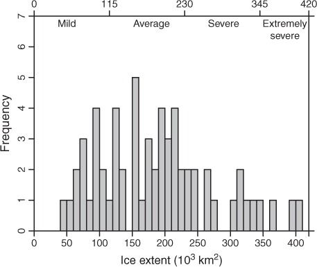
Winters can be sorted into ice severity classes on the basis of MIB observations. According to the present revised standards that correspond to the recent climate (Vainio, 2011), winters with an ice extent smaller than 115×10³ km² (or 27% of the total sea area) are classified as mild, those from 115 to 230×10³ km² (27–55%) as average and those from 230 to 345×10³ km² (55–82%) as severe. If the ice extent exceeds 345×10³ km², the winter is regarded as extremely severe. Since the smallest MIB observed thus far is 49×10³ km² (12%), winters with an even smaller ice extent than this are termed unprecedentedly mild.

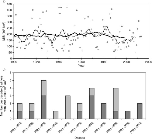
The variability of the sea ice cover in the Baltic Sea is a sensitive indicator of climatic fluctuations and changes in northern Europe. Several studies have reported a declining trend in MIB (Jevrejeva et al., 2004; Schmeltzer et al., 2008; Vihma and Haapala, 2009; BACC II Author Team, 2014). Considering the winters of 1901–2013, we did not, however, find any statistically significant linear trend in MIB (Fig. 1a) or in the decadal sums of severe and extremely severe ice winters (Fig. 1b). Instead, there were strong inter-annual and inter-decadal variations. A noteworthy feature is, nonetheless, the scarcity of extremely severe ice winters since the late 1980s.

Fig. 1 Past records of the Baltic Sea ice cover. (a) The annual maximum ice extent (MIB) in 1901–2013; (b) the number per decade of severe (dark grey) and extremely severe (light grey) ice winters, that is, winters with MIB exceeding 230×10³ km² or 345×10³ km², respectively, during 1901–2010. The dotted and solid curves in panel (a) show the 10 and 30 yr running means, respectively.

One of the most robust features of future climate projections is that the surface air temperature will increase within the Baltic Sea catchment area in winter (BACC II Author Team, 2014). A warming trend can be expected to directly impact the duration, thickness, extent and other properties of the sea ice cover, as well as the partitioning between snowfall and rainfall. Such changes in turn will have a major impact on oceanographic and hydrological conditions, the ecosystems, the biogeochemical cycles, coastal erosion, ice roads and winter navigation in the Baltic Sea.

Previous estimates of the sensitivity of the Baltic Sea ice cover to climatic changes have been based on numerical modelling (Omstedt and Nyberg, 1996; Haapala and Leppäranta, 1997; Omstedt et al., 2000; Haapala et al., 2001; Meier et al., 2004; Meier, 2006) or on using statistical methods to correlate sea ice variability to atmospheric conditions (Tinz, 1996; Omstedt and Chen, 2001; Jylhä et al., 2008; Luomaranta et al., 2010). In conjunction with projections of future warming, considerable thinning of the ice and shrinking of the ice cover, as well as a shortening of the ice season in the Baltic Sea, are foreseen in these studies, but there are differences in the strength of the responses. For example, Haapala et al. (2001) assessed a reduction of the mean MIB by one-third or a half by the late 21st century, the range corresponding to two regional ice-ocean models that had been run with equal future atmospheric forcing. In the works of Meier et al. (2004) and Meier (2006), two different scenarios for the concentrations of greenhouse gases (GHGs) and altogether four modelling systems were applied, the corresponding projected decreases in mean MIB ranging from a half to four-fifths. Despite these drastic reductions, no totally ice-free winters were simulated to occur during 2071–2100. In contrast, in a model experiment conducted by Omstedt et al. (2000), there was almost no ice in 3 out of 10 winters.

As regards statistical methods, Omstedt and Chen (2001) established a multiple regression equation that linked MIB to the large-scale atmospheric circulation. An exponential regression model between MIB and the mean air temperature from November to March was in turn developed by Tinz (1996) and updated by Jylhä et al. (2008) and Luomaranta et al. (2010). Based on that approach and on temperature projections derived from a set of global and regional climate model experiments, Jylhä et al. (2008) assessed MIB to become smaller than 80×10³ km² in the majority of years during 2071–2100. Using a subsequent (but not the most recent) generation of climate projections, Luomaranta et al. (2010) inferred that winters with an MIB larger than 280×10³ km² would be very improbable in 2041–2050.

In the papers referred to above, the differences in the responses of the Baltic Sea ice conditions arose from the divergent climate projections applied and the differences in numerical models or statistical approaches. Regional Baltic Sea circulation models, including the dynamics of the ice cover, are the most advanced tools to estimate the impacts of changes in the global climate system on a local scale, but due to the heavy computational requirements, their capacity to produce simulations under a wide ensemble of climatic forcing is limited. Conversely, statistical approaches cannot capture the real physical linkages among the various components of the climate system, but require very little computing resources compared to the numerical models. Statistical models are thus feasible tools for producing estimates of ice cover changes based on a large number of climate change scenarios. For example, it is possible to analyse a multitude of alternative temperature change projections produced by a wide ensemble of models forced by several greenhouse gas concentration scenarios.

In the present work, our objectives are to assess the temporal evolution of the Baltic Sea ice cover during the period 2021–2090 and to give an insight into the related uncertainties. We consider two sea ice quantities: the annual MIB and the climatological mean of the maximum fast ice thickness. Statistical methods are employed for both quantities: a non-linear regression model for the former and an analytical solution for the ice growth rate equation for the latter. Both approaches required projections of future changes in air temperature; these were based on data retrieved from the recently published global climate model (GCM) simulations within the Coupled Model Intercomparison Project Phase 5 (CMIP5, see Taylor et al., 2012). The CMIP5 simulations are forced by the new Representative Concentration Pathway (RCP) scenarios for GHGs and aerosol particles (Moss et al., 2010; van Vuuren et al., 2011); the simulations forced by RCP4.5 and RCP8.5 were selected for the present analysis.

In addition to the best estimates for changes in average sea ice conditions, derived from multimodel ensemble means, we explore three aspects not adequately addressed in previous studies: inter-annual variations, scatter across a multitude of climate models and the uncertainty induced by future GHG emissions. In order to consider inter-annual variability, frequency distributions of MIB in the future climate are constructed and three percentiles in them are considered. This allows us to compare the influence of climate change on winters that represent typical ice conditions versus those with very extensive or scant ice cover. Second, to assess the uncertainty associated with modelling differences, we examine the scatter of the responses produced by 28 individual models. Finally, the uncertainty induced by future emissions is considered by analysing the responses to two very divergent GHG scenarios.

2. Data and methods

2.1. Data

2.1.1. Ice and temperature observations.

Our observational data consisted of observations of annual maximum ice extent in the Baltic Sea in the years 1952–2012 and air temperature observations in the coastal area of the Baltic Sea during the same period. Furthermore, observations of the annual maximum ice thickness in 1971–2000 were available for Kemi (65.73°N, 24.55°E) and Loviisa (60.42°N, 26.27°E) (Jevrejeva et al., 2002).

Most of the observed MIBs in 1952–2012 can be classified as average ice winters (Fig. 2). The date refers to the year of January in each winter; that is, the first and last winters included in our study were the cold seasons of 1951–1952 and 2011–2012.

Fig. 2 The frequency distribution of the observed annual maximum ice extent in 1952–2012. The ice winter classification is shown along the upper horizontal axis showing the ice extent limits for mild, average, severe and extremely severe ice winters.

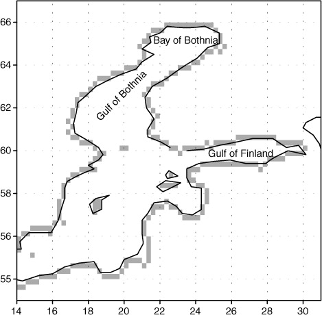
For air temperature observations on the coasts of the Baltic Sea, we used the E-OBS gridded dataset (Haylock et al., 2008) within the latitudes of 53–67°N and longitudes of 14–31°E (Fig. 3). The spatial resolution of the dataset was 0.25°, and the number of coastal grid points used here was 245. E-OBS version 7.0 was employed (except for the years 1951–1960 that were covered by version 6.0).

Fig. 3 The coastal grid points in the E-OBS gridded data set for the observational air temperatures. The positions of three of the sub-basins of the Baltic Sea are shown: the Bay of Bothnia, the Gulf of Bothnia and the Gulf of Finland.

2.1.2. Climate model output.

Climate model simulations of air temperature under the RCP4.5 and RCP8.5 scenarios (Moss et al., 2010; van Vuuren et al., 2011), extending until the end of this century, were downloaded from the CMIP5 archive. Of these two greenhouse gas scenarios, the RCP4.5 scenario is mid-range, in which the actions of climate policy are moderately effective. The RCP8.5 scenario, by contrast, represents very high emissions. In RCP4.5, the CO₂ concentration stabilises at around 540 ppm by the end of the century; in RCP8.5 the concentration at that time exceeds 900 ppm. The differences between the scenarios are small at the beginning of the study period, but increase over time.

Monthly mean temperature data for both the RCP4.5 and RCP8.5 scenarios were available for a total of 35 GCMs. However, models failing to meet three fundamental conditions were omitted from the analysis. First, two of the models (BNU-ESM and FGOALS-s2) were severely biased in simulating the sensitivity to recent past forcing, the simulated global mean temperature trend during the past 50 yr exceeding the observation-based estimate by more than 0.4°C. Second, in four models (FGOALS-s2, FIO-ESM, GFDL-ESM2G and HadGEM2-AO) the projected global mean temperature increase under the various RCP scenarios behaved inconsistently. For example, the global mean temperature response to the RCP8.5 forcing simulated by FIO-ESM was 2.7 times as large by 2070–2099 as the corresponding response to RCP4.5, while the multimodel median of that ratio was 1.8. Third, there were five models (BNU-ESM, CSIRO-Mk3-6-0, FGOALS-s2, FIO-ESM and IPSL-CM5B-LR) for which the simulated baseline-period climatological mean temperature and/or precipitation in Europe deviated markedly from their observational counterparts. Note that for some models there were several objections; for example, the FGOALS-s2 model failed to fulfil all three criteria.

Since the above-discussed seven models were disregarded, the present analysis is based on 28 GCMs in total (Table 1). For control purposes, however, we also calculated the multimodel mean temperature response to the RCP8.5 forcing as a mean of all the 35 models. The outcome proved to be nearly indistinguishable from the 28-model mean.

Table 1. The CMIP5 models used in this study

Model	Country of origin	Mean (i) (°C)	Range (ii) (°C)	Trend (iii) (°C/10 yr)	ΔT (°C):	RCP4.5	ΔT (°C):	RCP8.5
MIROC5	Japan	−3.4	26.5	0.41	2.8	(16)	2.9	(14)
MIROC-ESM	Japan	−0.4	22.0	0.28	3.2	(23)	3.9	(24)
MIROC-ESM-CHEM	Japan	−0.6	22.6	0.11	3.5	(25)	4.1	(25)
MRI-CGCM3	Japan	−4.1	20.3	0.21	1.8	(6)	2.8	(11)
BCC-CSM1-1	China	−5.1	20.7	0.72	2.6	(15)	3.7	(20)
INMCM4	Russia	−3.4	21.2	0.14	1.9	(8)	2.0	(2)
NorESM1-M	Norway	−1.4	18.8	0.19	2.4	(11)	2.6	(10)
NorESM1-ME	Norway	−1.2	18.7	0.17	2.0	(9)	2.8	(12)
HadGEM2-ES	UK	−3.4	22.4	0.38	2.8	(18)	3.4	(18)
HadGEM2-CC	UK	−6.1	24.8	0.34	2.8	(17)	3.9	(23)
MPI-ESM-LR	Germany	−2.3	20.1	0.34	1.8	(7)	2.6	(9)
MPI-ESM-MR	Germany	−2.4	19.7	0.34	2.4	(12)	2.4	(5)
CNRM-CM5	France	−3.6	24.8	0.56	2.5	(13)	3.1	(16)
IPSL-CM5A-LR	France	−6.7	27.2	0.42	4.0	(26)	4.6	(27)
IPSL-CM5A-MR	France	−3.5	23.7	0.42	3.2	(24)	3.0	(15)
CMCC-CM	Italy	−7.0	21.4	0.70	4.5	(27)	5.2	(28)
CMCC-CMS	Italy	−6.4	22.4	0.72	4.9	(28)	4.4	(26)
GFDL-CM3	USA	−1.2	17.4	0.46	3.2	(21)	3.8	(22)
GFDL-ESM2M	USA	−4.2	21.6	0.23	2.9	(19)	2.9	(13)
GISS-E2-R	USA	−6.0	25.6	0.39	2.5	(14)	3.8	(21)
GISS-E2-H	USA	−5.1	22.8	0.22	3.2	(22)	3.4	(17)
CCSM4	USA	−0.8	21.0	0.31	1.6	(4)	1.9	(1)
CESM1-CAM5	USA	−0.9	20.5	0.18	1.6	(3)	2.5	(8)
CESM1-BGC	USA	−0.4	20.5	0.59	0.8	(1)	2.5	(7)
CanESM2	Canada	−1.3	22.3	0.48	3.0	(20)	3.6	(19)
ACCESS1-0	Australia	−1.8	18.6	0.22	1.4	(2)	2.1	(3)
ACCESS1-3	Australia	−0.3	17.2	0.09	2.2	(10)	2.5	(6)
EC-EARTH	Several	0.0	16.6	0.27	1.7	(5)	2.4	(4)
28-model mean	−3.0	21.5	0.35	2.6	3.2
Observations	−2.4	21.3	0.48

Columns 3–5 show (i) the November–March mean temperature (°C), (ii) the annual temperature range (°C) and (iii) the trend (°C/decade) in November–March mean temperature, all calculated for the period 1961–2010. The November–March mean temperature change ΔT (°C) between the periods 1971–2000 and 2031–2060 is given separately for the RCP4.5 and RCP8.5 scenarios. All quantities are averaged over the coastal grid points. The ordinal numbers of the models, shown in parentheses, are determined by the magnitude of the projected temperature change (in ascending order) under these two scenarios. The countries involved in the development of the EC-EARTH model are Belgium, Denmark, Ireland, Italy, the Netherlands, Norway, Portugal, Spain, Sweden and Switzerland.

The climate model data were smoothed by applying a 30 yr running mean and interpolated onto the same 0.25° grid that was used for the observational temperatures. The November–March mean temperature change from 1971–2000 to 2031–2060, averaged over the coastal grid points (Fig. 3), differs from model to model (Table 1). In the RCP4.5 scenario, the change varies between 0.8 and 4.9°C, while in the RCP8.5 scenario the range is 1.9–5.2°C. In Table 1, the models are ordered according to their projected temperature response (shown in parentheses).

2.1.3. Evaluation of the model simulations.

Although the 28 GCMs selected behave reasonably on the large scale, biases may still exist on regional scales, resulting, for example, from a crudely resolved topography and land-sea distribution in the Baltic Sea and its adjacent areas. Hence, this sub-ensemble of the original set of 35 models was further evaluated by comparing the modelled temperature climate on the Baltic Sea coasts with its observational counterpart. The comparison covers the years 1961–2010, that is, the same period that was used as a baseline in deriving the statistical distributions of ice extent for the future time slices (section 2.2). Note that this evaluation was only made with respect to one variable (air temperature) and a limited area; it is not intended to be used for far-reaching inferences on the quality of the models in general.

In the model comparison, three quantities were examined: (1) the climatological long-term (50 yr) mean temperature in November–March, (2) the annual temperature range, that is, the 50 yr mean of July minus February temperature and (3) the 50 yr linear least-squares trend of the November–March mean temperature. All quantities are averages over the coastal grid points of the Baltic Sea (Fig. 3).

In studying the 28-model mean, quantities (1) and (2) proved to be simulated well, even though there was rather a large scatter across the models (Table 1). The observation-based November–March mean coastal temperature in 1961–2010 was −2.4°C. The corresponding multimodel mean is −3.0°C, with individual models simulating mean temperatures ranging from −7.0°C (CMCC-CM) to 0.0°C (EC-EARTH). For the annual temperature range, the corresponding values are 21.3°C (observational), 21.5°C (multimodel mean), 16.6°C (minimum among the GCMs) and 27.2°C (maximum). The modelled biases in quantities (1) and (2) bear a strong inverse correlation (Table 2), reflecting the fact that the simulated temperatures vary more strongly across the models in winter than in summer. Of these two variables, we therefore concentrate on exploring the November–March mean temperature (quantity (1)).

Table 2. Correlations between various temperature indices derived from the 28 GCMs listed in Table 1

Index	Range (ii)	Trend (iii)	RCP4.5	RCP8.5
November–March mean temperature (i)	−0.62	−0.48	−0.60	−0.61
Annual temperature range (ii)	0.30	0.45	0.47
November–March temperature trend (iii)	0.40	0.53

The indices representing the simulated recent past climate are (i) the November–March mean temperature, (ii) the annual temperature range, and (iii) the trend in November–March mean temperature, all calculated over the period 1961–2010. The index representing the future climate is the projected change in November–March temperature from the period 1971–2000 to 2031–2060; the correlations for this index are given separately for the RCP4.5 and RCP8.5 scenarios. Temperatures are averaged over the Baltic Sea coastal grid points (Fig. 3). Significance limits for the correlations: 0.37 (p=0.05), 0.48 (0.01), 0.59 (0.001).

As far as quantity (3) is concerned, the observation-based Baltic Sea coastal temperatures in 1961–2010 show a warming trend of 0.48°C/decade. The corresponding multimodel mean trend is 0.35°C/decade, while the trends simulated by individual models vary from 0.09 to 0.72°C/decade (Table 1). In total, 22 out of 28 models simulate trends that are weaker than observed. Nevertheless, this does not necessarily indicate that the models do in fact tend to underestimate the actual warming signal; in such a small area as the Baltic Sea the observed trend may be severely affected by noise originating from natural climatic fluctuations. In fact, there was a distinct jump in the time series of winter temperatures around the year 1988, with cold winters occurring much more frequently before than after that year. The discontinuity is apparent in the ice extent observations as well (see Fig. 1a).

Several previous studies (see Bracegirdle and Stephenson (2013) and references therein) have suggested that models simulating a cold bias in baseline climate have a tendency to produce large future temperature responses in high latitudes, particularly close to the sea ice edge. Here, we discuss the relation between the model biases and their projections of future temperatures under the RCP8.5 scenario. The conclusions also hold for RCP4.5, even though the correlations are somewhat weaker (see Table 2). In the model ensemble, there is a significant positive correlation (r≈0.5) between the modelled past (1961–2010) trends and the changes projected from 1971–2000 to 2031–2060. Moreover, both quantities correlate negatively (r≈−0.5 to −0.6; Table 2) with the modelled bias of the November–March temperature. In part, this may be explained by local feedback phenomena. Models producing too low winter temperatures typically simulate sea ice and snow cover in excess, the resulting large albedo and effective thermal isolation further strengthening the coldness. As climate warms, this cooling effect is mitigated, leading these models to simulate strong increases in temperature. In other models with high baseline temperatures, this feedback works less effectively.

Using all the 28 models included in the analysis, the multimodel mean temperature response to the RCP8.5 forcing for the 2040s was 3.2°C. We next studied the influence of further reducing the ensemble size by excluding models with a lower performance, that is, the three models simulating the largest positive and the three producing the largest negative bias in mean temperature. As a consequence, the multimodel mean temperature response would only be reduced by 5%, but the scatter among the modelled responses would be diminished by 23%. A less drastic elimination, only omitting those three models producing the largest bias in absolute terms (in all of them, the bias was negative), would reduce the multimodel mean temperature response by 6% and the standard deviation by 21%. Accordingly, disregarding the models having the largest difficulties in simulating the recent past climate in the target area would not substantially affect the best-estimate (multimodel mean) temperature response, but the apparent uncertainty interval would be curtailed appreciably.

At first sight, any prospect of narrowing the uncertainty interval sounds beneficial. Nonetheless, as shown by Huybers (2010), the various feedback effects (cloud, albedo and the combined water vapour plus lapse rate) tend to co-vary negatively in the GCM ensemble. This kind of compensation between the feedbacks may spuriously curtail the inter-model spread of climate sensitivity. Therefore, in order to avoid the risk of determining too small error bars for the Baltic Sea ice projections, it was decided in this work to accept for analysis all the 28 models showing reasonable skill in simulating the present past climate.

2.2. Methods

2.2.1. Annual maximum ice extent.

Broadly following Tinz (1996) and Jylhä et al. (2008), we fitted a non-linear regression model to the observed November–March mean temperature and annual maximum ice extent data for the years 1952–2012 (Fig. 4). The regression equation is given by:1

Fig. 4 The regression model for the ice extent. The model was fitted to the observed annual maximum ice extent and the November–March mean temperature at coastal grid points in 1952–2012. Some winters with a very high or low value of air temperature or ice extent are annotated. The date refers to the month of January in each winter.

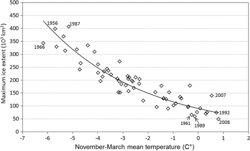
where MIB is the annual maximum ice extent (km²) and T is the November–March mean temperature (°C) averaged over the coastal grid points. Based on the data, the following values were derived for the coefficients: A=(90.2±4.2)×10³ km² and B=(0.253±0.015) (°C)⁻¹. The coefficient of determination of the model, R ², is 82.8%. At T=−3°C, the error in MIB due to the standard errors of the coefficients A and B is about 10%, and from −1 to +1°C about 5%.

The regression model [eq. (1)] was applied to project the probability distributions of MIB during the coming decades of this century. At first, a sample of size 50 was constructed to represent November–March temperatures T for each decade. This was produced by adding the GCM-based temperature increases ΔT for the decade in question to the observed values of T in the years 1961–2010 (a delta-change method). In order to reduce random effects, ΔT for each decade was calculated as a 30 yr mean, centred on that decade. For example, the mean temperature change for the period 2011–2040 represents the decade 2021–2030. Next, using these samples of T in eq. (1), we produced artificial frequency distributions of MIB for the seven future decades in the period 2021–2090. Finally, we determined three percentiles of the MIB distributions: the 5th (lower tail), 50th (median) and 95th (upper tail), the first and the third roughly corresponding to values that are fallen short of or exceeded, respectively, on average once in 20 yr. In 9 out of 10 yr, MIB can be expected to remain between the 5th and 95th percentiles.

The calculations were performed for each climate model listed in Table 1 and for both RCP scenarios. This enabled us to assess the uncertainty in MIB caused by the differences in the GHG scenarios and by the scatter of the temperature responses in the various GCMs. In order to obtain the best estimates for the long-term trends in the three percentiles of MIB, we also derived their 28-model averages. The model uncertainty assessment focused on the decade 2041–2050. This decade was selected for three reasons. First, it is sufficiently distant to exhibit a clear climate change signal compared to the noise due to internal climate variability. Second, it is sufficiently near not to be disturbed by a simplification made in our calculations, that is, the omission of potential changes in the inter-annual variability of winter temperatures. This omission mainly affects results at the end of the century, an issue to be discussed later. Third, an insight into the reliability of the sea ice projections for the first half of this century is of the highest relevance for many practical applications, such as designing fleets of icebreakers.

2.2.2. Sea ice thickness.

The 30 yr mean of the annual maximum fast ice thickness was assessed using an analytical solution for the thermodynamic ice growth equation that is based on the sum of freezing degree-days (Stefan, 1890; Zubov, 1945; Leppäranta, 1993):2 where a=3 cm(°C×d)^−1/2, d=10 cm and S is the annual cumulative sum (°C×d) of daily mean air temperatures below 0°C (freezing degree-day sum). The approach, the so-called FDD model, is suitable for assessing ice thickness during the ice growth phase, up to an annual maximum value of h, but is no longer valid when the ice is melting (Stefan, 1890).

Our method of estimating the freezing degree-day sum S in eq. (2) was based on local monthly mean temperatures. We first multiplied the negative monthly mean temperatures in Celsius by the number of days in the month to get an approximation for the monthly freezing degree-day sums. The sum of the contributions of all months with a sub-zero mean temperature, that is, S in eq. (2), was then used to obtain the maximum ice thickness h.

For the baseline period 1971–2000, we used the observed monthly 30 yr mean temperatures to compute S and thereby h. The climatological monthly mean temperature for a future decade was obtained by adding the GCM-based 30 yr mean temperature response, centred on the target decade, to the observational baseline-period temperatures. The temperature projections were calculated separately for each individual GCM and, in addition, as 28-model means. Our results for the climatological maximum ice thickness h thereby represent responses to a range of individual temperature projections as well as to their average.

The FDD model [eq. (2)] does not take into account the snow layer lying on top of the ice cover. Ice thicknesses are thus systematically overestimated by up to 40 cm, and the value of h resulting from the model can be considered as the upper limit for ice growth in a typical winter (Leppäranta, 1993). The present approach is only valid for the coastal fast ice, since in the drift ice regions, sea ice thickness depends substantially on the dynamical processes like rafting and ridging (Vihma and Haapala, 2009). Furthermore, as the E-OBS gridded dataset does not cover air temperatures over sea areas, the ice thickness could only be assessed in coastal areas.

The 30 yr means of the observed maximum fast sea ice thickness at Kemi and Loviisa in 1971–2000 were 75 and 38 cm, respectively. The corresponding values of h based on eq. (2) are 98 and 66 cm, respectively, implying an overestimation of 24 cm (32%) for Kemi and 28 cm (74%) for Loviisa. The insulating effect of snow-on-ice, ignored here, is presumably the main reason for this overestimation. Additionally, the exact locations of the ice thickness observation sites may have changed in time during the 30 yr period, which may have influenced the quality of the observational time series. At Loviisa, the proximity of a nuclear power plant, with its condensation water having a warming effect, may also be seen in the ice thickness statistics.

3. Results

3.1. Annual maximum ice extent

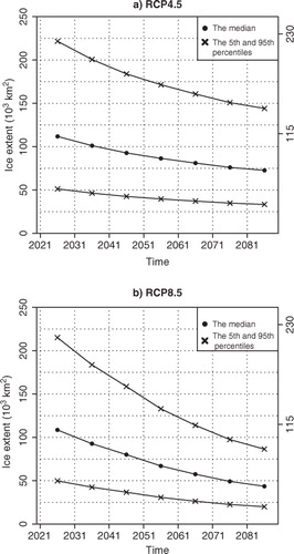
We first focus on the ensemble-mean changes in the distribution of the annual maximum ice extent. Three percentiles (95th, 50th and 5th) were derived from the artificial 50 yr samples that were produced for each decade of the period 2021–2090. The 95th percentile, representing winters with an uncommonly wide ice cover, is projected to diminish faster than the median or the 5th percentile (Fig. 5). The linear trends under the RCP4.5 scenario for the three quantities are −12 700 km²/10 yr, −6400 km²/10 yr and −2900 km²/10 yr, respectively. The decline is faster under the RCP8.5 than the RCP4.5 scenario, in accordance with the more ample warming in the former scenario. The corresponding linear trends in the percentiles for RCP8.5 are −21 600 km²/10 yr, −10 900 km²/10 yr and −5000 km²/10 yr, respectively. If the RCP8.5 scenario is realised, average ice winters, according to the current standards, would be very exceptional from the 2060s onward, but under the RCP4.5 scenario the 95th percentile of MIB falls to that category even in the 2080s. Under both scenarios, the probability of unprecedentedly mild ice winters will increase during the study period. In the RCP8.5 scenario, even the median MIB would belong in that category from the 2080s onward.

Fig. 5 Temporal evolution of the annual maximum ice extent during the course of this century. The estimates are given separately for the median values, representing a typical winter (line with dots), and for the 5th and 95th percentiles, corresponding to scant and widespread ice cover (lines with crosses). All the results are ensemble means of sea ice projections, derived from temperature responses of 28 individual CMIP5 models (Table 1). The vertical axis on the right shows the upper class limits for mild and average ice winters, according to current standards. The limit for unprecedentedly mild winters is 49×10³ km². (a) The RCP4.5 scenario, (b) the RCP8.5 scenario.

We next address the uncertainty caused by different temperature responses in the various GCMs, first discussing the inter-model scatter of the medians of MIB. The median values decreased in time in all model projections, faster so in the RCP8.5 scenario than in RCP4.5. For RCP8.5, the inter-model range of median MIB became smaller during the study period, with the standard deviation of the medians decreasing from 19 000 km² in the 2020s to 14 000 km² in the 2080s. The standard deviation under RCP4.5 was larger than under the RCP8.5 scenario, ranging over the whole period between 19 000 and 22 000 km² without any clear temporal trend. The smaller scatter among the model projections in the RCP8.5 than in the RCP4.5 scenario is, however, less evident when the normalised standard deviations (or coefficients of variance) of the medians are considered.

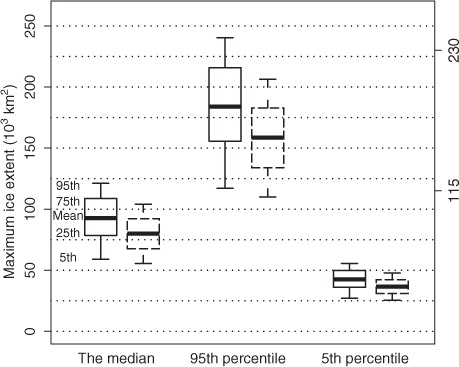
The multimodel means and the inter-model scatter for all three percentiles of MIB are exemplified for 2041–2050 in Fig. 6. The mean median value for the RCP4.5 scenario is about 93×10³ km² and for RCP8.5 about 80×10³ km² (see also Fig. 5). For the RCP8.5 scenario, there is a strong consensus among the model projections that the median MIB falls into the class of mild ice winters. For RCP4.5, most of the models likewise agree with that. The scatter is wider for the 95th percentile, representing winters with a more widespread ice cover. For most of the model projections, this high percentile belongs to the class of average ice winters. However, according to the model ensemble, there is a small probability for the upper tail of the MIB distribution to be classified as a severe ice winter in RCP4.5, or as a mild ice winter in RCP8.5. The scatter is smallest around the 5th percentile, representing the lower tail of the MIB distribution. All the models are strongly unanimous in the 5th percentile belonging to the class of mild or even unprecedentedly mild ice winters. Inferring from the observations performed thus far, in the mild winters of the 2040s, ice only occurs in the Bay of Bothnia and perhaps in the eastern Gulf of Finland.

Fig. 6 Inter-model scatter and inter-annual variability of the annual maximum ice extent in 2041–2050. The median and the 5th and 95th percentiles (the horizontal axis) demonstrate inter-annual variability and the box-and-whiskers plots illustrate inter-model scatter. Within each box, the thick solid line refers to the 28-model mean ice extent, also shown in Fig. 5. The box depicts the upper and lower quartiles of the sea ice projections, whiskers the 5th and 95th quantiles. The boxes drawn with solid lines show the RCP4.5 scenario and those with dashed lines RCP8.5. The vertical axis on the right shows the upper class limits for mild and average ice winters. The limit for unprecedentedly mild winters is 49×10³ km².

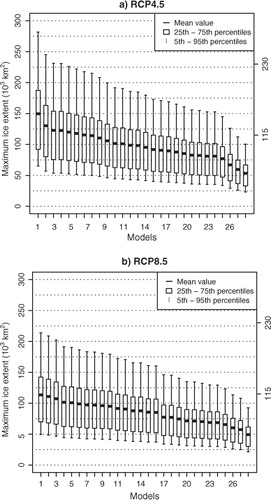
Finally, we consider MIB in 2041–2050 separately for each ensemble member (Fig. 7). In that decade under the RCP4.5 scenario, the model with the weakest warming (Table 1) and thereby the largest mean MIB is CESM1-BGC; this model produces the widest range between the 5th and 95th percentiles (Fig. 7a). The model projecting the strongest warming (Table 1), CMCC-CMS, is that also producing the smallest mean MIB and the narrowest range. In RCP8.5 (Fig. 7b), the corresponding extreme models are CCSM4 (the largest MIB) and CMCC-CM (the smallest MIB). Under the RCP4.5 scenario, the mean MIBs derived from the temperature responses of seven models (25% out of the total number) can be classified as average, the rest of the model-based estimates belonging to the class of mild ice winters. The 95th percentiles of four models can be classified as severe, and the 5th percentiles of 21 models as unprecedentedly mild. Under the RCP8.5 scenario, the mean values of all models fall into the class of mild (but not unprecedentedly mild) ice winters, and none of the 95th percentiles exceeds the class limit of a severe ice winter.

Fig. 7 The annual maximum ice extent (MIB) in 2041–2050 according to each individual GCM. The numbers on the horizontal axis show the GCMs in ascending order of the projected November–March mean temperature response (for identifying the models, see Table 1). The short black line inside a box denotes the mean value of the distribution, the boxes the 25th and 75th percentiles and the whiskers the 5th and 95th percentiles of inter-annual variability for each model. The vertical axis on the right shows the upper class limits for mild and average ice winters. (a) RCP4.5, (b) RCP8.5.

3.2. Ice thickness

The mean annual maximum fast ice thickness for the whole study area was examined as a response to the 28-model mean temperature projection in two future decades, 2041–2050 and 2081–2090. In addition, the results based on the individual model projections were calculated for the whole study period at three locations: Kemi, representing the coast of the Bay of Bothnia; Loviisa, representing the eastern Gulf of Finland; and Vilsandi (58.38°N, 21.82°E), representing the Baltic Sea Proper (for the locations, see Fig. 8a).

Fig. 8 The annual maximum coastal sea ice thickness (cm) in typical past and future winters. The calculations with the FDD method are based on (a) observed temperatures in 1971–2000 and (b–e) the 28-model mean temperature projections under the two RCP scenarios for two future decades. The crosses denote the locations of Kemi, Loviisa (Lov) and Vilsandi (Vil).

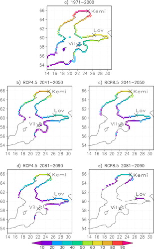
When applied to the observed temperatures of the baseline period 1971–2000, the FDD model [eq. (2)] implied that most of the coastal areas become ice-covered in a typical contemporary winter (Fig. 8a). The resulting mean maximum ice thickness varies substantially, being locally more than 90 cm in the Bay of Bothnia and only 0–10 cm in the south-western parts of the Baltic Sea.

The mean maximum ice thickness is projected to decrease in coming decades (Fig. 8b–8e). Based on the 28-model mean temperature projections, for the northern coast of the Bay of Bothnia in 2041–2050, the ice thickness is about 60–80 cm under the RCP4.5 scenario (Fig. 8b) and about 50–70 cm under RCP8.5 (Fig. 8c). The differences between the scenarios increase by the end of the study period. In 2081–2090 under RCP4.5, the ice thickness in the Bay of Bothnia may locally still exceed 60 cm, whereas elsewhere in the Gulf of Bothnia and in the Gulf of Finland it is 10–40 cm (Fig. 8d). According to the RCP8.5 scenario, most of the Baltic Sea is projected to be ice-free in 2081–2090 (Fig. 8e). In the northernmost Bay of Bothnia, however, h is then mainly 20–40 cm. This indicates that even if the high-emission RCP8.5 is realised, in a typical winter the Baltic Sea is unlikely to become totally ice-free during this century.

The linear trends in h, derived from the 28-model mean temperature projection under the RCP4.5 scenario, were −3.4 cm/10 yr, −3.3 cm/10 yr and −1.0 cm/10 yr for Kemi, Loviisa and Vilsandi, respectively (Fig. 9a). The inter-model standard deviation in the projected ice thickness in 2021–2030 was 6 cm at all three sites. At Kemi and Loviisa, the deviation increased to 15 cm and 11 cm, respectively, by the end of the study period. The southernmost location of the three, Vilsandi, already remains ice-free in the first decade, 2021–2030, according to six of the 28 models. In the last decade 2081–2090, the temperature projections of only five models allow the formation of ice there. In contrast to Kemi and Loviisa, the standard deviation at Visandi decreased towards the end of the period, being only 2 cm in 2081–2090.

Fig. 9 Temporal evolution of the mean maximum ice thickness at three locations during the course of this century. The ice projections for Kemi (dots), Loviisa (crosses) and Vilsandi (triangles) are based on the temperature responses of the individual GCMs. The short horizontal lines show the mean values of all the model-based projections for each decade. Note that the position of the symbols within each decade is slightly shifted to make the figure more readable. (a) RCP4.5, (b) RCP8.5.

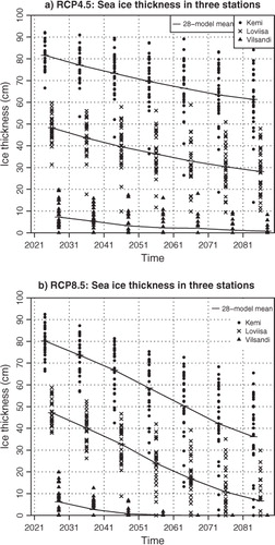
The thinning of the ice is faster in the RCP8.5 scenario (Fig. 9b) than in RCP4.5. The linear trends of the ice thickness for Kemi, Loviisa and Vilsandi are now −7.6 cm/10 yr, −7.0 cm/10 yr and −0.8 cm/10 yr, respectively. The zero-values at Vilsandi in the last three decades made the trend notably weaker there than at Kemi or Loviisa. At Kemi, the inter-model standard deviation of the mean maximum ice thickness increased from 7 to 19 cm during the study period. At Kemi, two of the 28 modelled temperature projections produced no ice for a typical winter in 2081–2090. At Loviisa, the corresponding number was 15 of the 28 models. The ice cover for an average winter disappears at Vilsandi in 2061–2070, as it stays ice-free according to the temperature projections of all the models in the last three decades. This does not, however, mean that sea ice cannot occur at Vilsandi at all in the late 21st century. Our results for the ice thickness portray climatological means, but do not provide inter-annual variations.

As mentioned earlier, due to the calculation method these results should be considered as an upper limit for the ice growth in a typical winter (Leppäranta, 1993). Because of this tendency towards an overestimation in the absolute values of h, we also considered the percentage changes relative to the period 1971–2000. When derived from the 28-model mean temperature projections, the decline in 2041–2050 would be about 25–30% at Kemi and 40–50% at Loviisa, only weakly depending on the RCP scenario (Table 3). In 2081–2090, the ensemble-mean change at Kemi is about 40% under RCP4.5 and about 60% under RCP8.5. Further southwards, the projected percentage changes are stronger, that is, 60–90% at Loviisa and up to 100% at Visandi. Apart from Visandi under RCP8.5, however, the ranges of the responses derived from the individual GCMs are considerable. In the 2040s at Loviisa, for example, the uncertainty range is 20–67% when both RCP scenarios are taken into account (Table 3).

Table 3. The projected percentage reductions in the mean maximum ice thickness (h)

Observation	RCP4.5		RCP8.5
1971–2000 (cm)	2041–2050 (%)	2081–2090 (%)	2041–2050 (%)	2081–2090 (%)
Kemi	75	25 (16–44)	37 (19–59)	32 (18–50)	63 (40–99)
Loviisa	38	40 (20–63)	57 (32–81)	50 (34–67)	89 (64–100)
Vilsandi	88 (46–100)	97 (81–100)	97 (80–100)	100

The best estimates for the declines from the period 1971–2000 to the decades 2041–2050 and 2081–2090 are based on the 28-model mean temperature projections under the RCP4.5 and RCP8.5 scenarios. The 90% confidence intervals, derived from the inter-model differences in the temperature responses, are given in parentheses. The 30 yr mean values of the observed annual maximum ice thickness in 1971–2000 at Kemi and Loviisa are shown in Column 2.

4. Discussion

4.1. Causes of uncertainties

The wide uncertainty ranges in our results are caused by differences in the climate models employed to produce the temperature projections, by the two different RCP scenarios and by internal climate variability. Owing to the large number of climate models used, the uncertainty related to model formulation could be estimated rather reliably. It appeared that the inter-model spread of temperature responses would be reduced appreciably if six out of 28 models, that is, those showing the lowest performance in simulating the observed climate, were omitted (Section 2.1.3). However, Huybers (2010) argued that GCMs in general rather under- than over-estimate the uncertainty of climate sensitivity. As previously mentioned, we therefore decided to retain all of the 28 models in order to avoid the risk of estimating too small error bars for the Baltic Sea ice projections.

Besides the issues mentioned above, some additional uncertainties arise from the calculation methods used in this work. For the estimates of the future ice extent, the exponential regression model [eq. (1)] had to be extrapolated outside the temperature range that was used to establish it. The model uses the average November–March temperature over the whole coastal Baltic Sea. Since it is possible to have freezing temperatures and sea ice in some parts of the study area (particularly in the north) and, at the same time, a considerably warmer winter elsewhere, the model produces non-zero ice extent even for spatially averaged temperatures above 0°C, in accordance with the observations (Fig. 4). But, because of its exponential form, the model actually never gives a zero MIB. Even with unrealistically high temperatures, it still would produce a small area of ice. On the other hand, the uncertainty related to the regression equation is relatively small compared to the inter-GCM scatter. For the 2080s, the error in MIB due to the standard errors of the regression coefficients is about 5000 km², whereas the inter-model standard deviation of the medians of MIB is 14 000 km² for RCP8.5 and even larger for RCP4.5. Even so, with the climate change continuing, higher temperatures will evidently occur, and the regression equation should be revised accordingly.

The delta-change method that we have used in constructing the probability distributions of the average coastal November–March temperatures for future decades assumes that the shape and width of the distribution remain unchanged. In particular, any possible changes in the inter-annual temperature variability are not taken into account. In near-term temperature projections, this simple constant delta-change method is found to be a reasonable approach (Räisänen and Räty, 2013; Kämäräinen, 2013). However, for projections targeted to the end of the century it would probably be beneficial if a method that includes changes in both the average values and the inter-annual variability were employed.

As mentioned earlier, the FDD model [eq. (2)] does not take into account the snow cover on the top of the ice. This causes an overestimation of up to 40 cm in the ice thickness estimates (Leppäranta, 1993). Despite a general decreasing trend in snow (Räisänen and Eklund, 2012), a similar bias exists to some degree in estimates of h both in the current and the future climate. We can therefore assume that the magnitude of the change is a fair estimate, perhaps more so in percentage terms (Table 3). Another feature related to eq. (2) is that our method of estimating the freezing degree-day sum S on the basis of monthly mean temperatures is somewhat inaccurate. Only months with a negative mean temperature were taken into account. For example, at the beginning of March, the month typically having the thickest ice cover in the Gulf of Finland (SMHI and FIMR, 1982), there may be sub-zero temperatures that still favour ice growth. This increase in the ice thickness is ignored in calculations of h, if a warm period later on during the month causes the monthly mean temperature to rise above zero. The impact of this error source is, however, reduced by the fact that the annual maximum ice thicknesses were examined as 30 yr mean values.

Important factors that could not be taken into account in this study are possible changes in precipitation, wind and ocean salinity. Based on the GCMs in Table 1, we assessed that in our study area the winter mean precipitation would increase by 20–31% under RCP8.5 by the 2080s. Both directly and through river runoff, this may affect salinity, and thereby the growth of ice. Because wind conditions control ice dynamics, potential changes in windiness are also of relevance. Wind speeds, especially in storms, have a large impact on the sea ice thickness distribution in drift ice regions, where ridging and new ice production in the leads may double the mass of thermodynamically produced ice (Vihma and Haapala, 2009). Besides wind speed, wind direction should also be considered. The prevailing wind direction determines in which coastal regions of the Baltic Sea ice ridging and compression predominantly occur. South-westerly to north-westerly winds increase the need for ice-breaking near the harbours of Finland and Russia, whereas easterly to northerly winds are likewise influential in Sweden and Estonia. However, the differences in responses between the current and the previous generation of GCMs make the projections for wind in the Baltic Sea area far more uncertain than those for temperature and precipitation. According to previous estimates for the winter season (November–March), both mean and extreme wind speeds would increase by approximately 2–5% by the end of this century (Gregow et al., 2012). On the other hand, our preliminary CMIP5-based calculations for monthly mean wind speeds, without investigations into extremes, only suggest a large inter-model scatter but no significant multimodel mean response.

4.2. Comparison to previous studies

The annual maximum Baltic Sea ice extent and thickness in the future have been a subject of several earlier studies. However, the surveys are not completely comparable, as they were based on different generations of climate models and GHG scenarios, analysed different time ranges or reported diverse aspects of the results. In the following, we compare our findings for the late century to the outcomes of the studies by Haapala et al. (2001), Meier et al. (2004) and Meier (2006); they used numerical sea ice models to estimate future changes in the Baltic Sea. Comparisons for the middle of the century are made between the present work and Luomaranta et al. (2010).

In the study by Haapala et al. (2001), two coupled ice-ocean models were applied to simulate ice conditions during two 10 yr periods, one representing pre-industrial atmospheric conditions and the other a climate generated by a 150% increase in the CO₂ concentration. Meier et al. (2004) employed a regional atmosphere–ocean climate model driven by two GCMs, both forced by the SRES A2 and B2 scenarios. Two 30 yr time slices were considered: 1961–1990 and 2071–2100. Meier (2006) widened the investigation by including four additional experiments that were conducted with a regional ocean climate model. The simulated mean MIB during the late 21st century varied between (117–190)×10³ km² in Haapala et al. (2001) and between (48–113)×10³ km² in Meier et al. (2004) and Meier (2006), depending on the modelling system and the GHG scenario. In the present work, for comparison, the multimodel average for the median MIB in the 2080s under the RCP4.5 and RCP8.5 scenarios was 73×10³ km² and 44×10³ km², respectively (Fig. 5).

In order to cursorily view to what degree the deviations in the results for MIB may be explained by divergent GHG scenarios, we now focus on multimodel mean percentage changes (Table 4). By examining percentage changes, the influence of model biases both in numerical and statistical studies can be alleviated. The scenarios were ordered based on the corresponding multimodel mean global temperature changes. For the 2040s, the responses to the RCP4.5 forcing scenario, derived in the current work, were very close to those presented by Luomaranta et al. (2010). For the 2080s, it appeared that the decrease in MIB was clearly weakest in the work by Haapala et al. (2001). Based on the remaining studies, the percentage declines in typical and high values of MIB tended to strengthen with increasing degree of global warming. For low values of MIB, representing winters with only a minor ice cover, the differences across the GHG scenarios were less evident (Table 4). Note, however, that the ensemble sizes diverged a lot between the studies, which hinders us from making robust inferences. Besides, the definitions of the low and high values of MIB given in the studies were not exactly equivalent.

Table 4. The projected percentage changes in the annual maximum ice extent (MIB) and the mean maximum ice thickness (h)

Scenario	Global ΔT (°C)	Ensemble size	Low	MIB (%) typical	High	h (%) Mean	Reference
Mid-century (2040s)
RCP4.5	1.4	28	−47	−46	−47	−25	This study
SRES A1B	1.4	19	−49	−44	−47	Luomaranta et al., 2010
RCP8.5	1.8	28	−55	−53	−54	−32	This study
Late century (2080s)
RCP4.5	2.1	28	−58	−58	−59	−37	This study
SRES B2	2.5	4	−81	−58	−51	−50	Meier et al., 2004; Meier, 2006
150%^a	2.6^b	2	−74	−44	−42	−42	Haapala et al., 2001
SRES A2	3.3	4	−88	−70	−65	−60	Meier et al., 2004; Meier, 2006
RCP8.5	3.7	28	−76	−74	−75	−63	This study

The multimodel mean responses by the 2040s and 2080s under various GHG scenarios are based on previous studies and the current work. The multimodel global mean temperature change (ΔT) is derived directly from the GCMs used (this work and Luomaranta et al. (2010)) or, for the dynamical downscaling experiments, is obtained from the references for the driving GCMs (the other studies). Low, typical and high MIB refer to the 5th, 50th and 95th percentiles of inter-annual variability, respectively (this work), or to the minimum, mean and maximum values during the simulation period. The results for h refer to Kemi (this work) or the centre of the Bay of Bothnia.

^a150% increase in the atmospheric CO₂ concentration, compared to pre-industrial conditions. ^bRäisänen et al. (2001).

Sensitivity studies performed by Meier et al. (2004) and Meier (2006) showed that severe ice winters are more responsive to the warming climate than are mild ones. This is also seen in our results shown in Fig. 5, where the rate of decrease of the 95th percentile is, in absolute terms, faster than that for the median or, especially, for the 5th percentile. In percentage terms, however, the changes for winters with scant ice cover are comparable (our study) or even larger than for winters with a more widespread ice cover (Table 4).

In the present paper, the mean annual maximum ice thickness (h) was only estimated in the coastal areas of the Baltic Sea. In the work by Meier et al. (2004), an assessment was made of h in the centre of the Bay of Bothnia (65°N 27′, 23°E 33′) for 2071–2100. The mean ice thickness there decreased from 58 cm to 23–39 cm, that is, 50–60%, depending on the scenario (Table 4). According to Haapala et al. (2001), the mean annual maximum ice thickness at the same location at the end of the century would be 27–43 cm, depending on the modelling system used. The two-model mean corresponded to a relatively modest percentage reduction of 42%, consistent with the moderate decline in MIB (Table 4). In our work, the RCP4.5 scenario produced a 28-model mean thickness of 61 cm for Kemi in 2081–2090. According to the RCP8.5 scenario, the corresponding thickness was 36 cm. The percentage declines were 37 and 63%, respectively (Table 4). Despite the differences in the study locations, the coastal area on the one hand, and the open sea, considered by Meier et al. (2004), on the other, the results are in good agreement. The differences among the GHG scenarios are clear. It can be inferred from Table 4 that, owing to two very divergent GHG scenarios and a multitude of alternative GCM-based temperature projections for both scenarios, the uncertainty in future ice thickness could be estimated more comprehensively in the current work than in the previous studies.

4.3. Consequences of a mainly ice-free Baltic Sea

According to our results for the RCP8.5 scenario, most of the Baltic Sea would be ice-free in the typical winters of the 2080s (Fig. 8e), the ensemble-mean estimate for the annual maximum ice extent ranging between about 20 and 85×10³ km² (or 5–20% of the total sea area) on an average in nine out of 10 yr (Fig. 5b). The decreases in ice cover will affect the ecosystems in the Baltic Sea. For example, the Baltic ringed seal, breeding on the ice, will probably lose many of its southern breeding habitats. In 2071–2100, the breeding of the Baltic ringed seal will be most likely to succeed in the Bay of Bothnia only (Meier et al., 2004). If the Baltic Sea, excluding the Bay of Bothnia, becomes ice-free during early spring by the end of the century the spring bloom of phytoplankton will start and end notably earlier (Eilola et al., 2013). Another consequence of the early ice break-up is that the mean significant wave height in spring will increase by 30 to 50 cm in many areas of the Gulf of Finland and the Gulf of Bothnia (Eilola et al., 2013).

Some consequences of the future loss of ice for the human activities are positive. The shipping in the area will benefit from the longer ice-free period, and the ice-breaking assistance will probably only be needed in the northern and the most eastern parts of the Baltic Sea (Haapala et al., 2001). However, when the sea remains ice-free, wave damage on the coastline may become more severe during winter storms. Wintertime cold outbreaks over an ice-free gulf with warm surface water (for example the Gulf of Finland) may cause intense snow showers in coastal areas (Savijärvi, 2012) presenting challenges to the maintenance of road networks and towns.

5. Conclusions

In this work, we have estimated future changes in the annual maximum sea ice extent and the mean maximum coastal sea ice thickness in the Baltic Sea under the RCP4.5 and RCP8.5 scenarios. The ice cover projections were based on temperature responses produced by 28 CMIP5 GCMs that showed reasonable performance in simulating the recent past climate in the Baltic Sea area. The sea ice projections were examined both as an ensemble-mean and separately for individual GCM-based temperature projections.

The annual maximum ice extent was estimated by a non-linear regression model, which was fitted to the observed values of wintertime temperature and annual maximum ice extent in the years 1952–2012. Applying this regression model to the GCM-based temperature projections, we derived frequency distributions for annual maximum ice extent for seven future decades within the period 2021–2090. According to both RCP scenarios studied, the annual maximum ice extent was found to decrease markedly. According to the RCP8.5 scenario, virtually only mild ice winters (ice extent < 115×10³ km²) occur from the 2060s onwards. Under RCP4.5, the decline of the ice extent is slower: average ice winters (ice extent between 115×10³ km² and 230×10³ km²) may still occur even in the 2080s.

The mean maximum sea ice thickness in coastal areas was assessed based on the sum of freezing degree-days. As expected, the decrease in ice thickness is faster in the RCP8.5 than in the RCP4.5 scenario. According to RCP8.5, in a conventional winter of the 2080s, sea ice would only occur in the Bay of Bothnia, with a maximum ice thickness of 30–40 cm, and in the north-eastern parts of the Gulf of Finland, with an ice thickness of 0–10 cm. According to RCP4.5, the coastal areas of the Gulf of Bothnia and the Gulf of Finland will still be ice-covered in the 2080s. Maximum ice thicknesses, locally exceeding 60 cm, would be found in the Bay of Bothnia.

Uncertainties in the results arise partially from the statistical calculation methods that we used in this work. On the other hand, since the statistical approaches required very little computing resources, we were able to incorporate a large number of different climate change scenarios. The spread among the changes derived from individual climate models appeared to be rather large. This suggests that when regional Baltic Sea circulation models are used to assess the impacts of climate change on ice cover, it would be necessary to employ the wide range of boundary conditions provided by a number of different climate models in order to adequately quantify the uncertainty in the estimates.

Despite the scatter in the rate of the projected changes, no uncertainty prevails about the direction of the long-term trend in sea ice. We conclude that sea ice will significantly decrease during this century. Although the Baltic Sea is unlikely to become totally ice-free in the typical winters of these coming decades, it is evident that the consequences of the ice reduction for ecosystems and communities will be notable.

6. Acknowledgements

This work was partially funded by the Academy of Finland through the ClimNext (no. 127239) and the MARISPLAN/FICCA (No. 140828) projects. Climate model data were downloaded from the Earth System Grid Federation data archive (http://pcmdi9.llnl.gov). Climate modelling groups (models listed in Table 1 of this paper) are acknowledged for providing the model output, and the World Climate Research Programme's Working Group on Coupled Modelling for maintaining the archive.

References

- BACC II Author Team. Series: Regional Climate Studies. Second BALTEX Assessment of Climate Change for the Baltic Sea Basin. 2014; Berlin: Springer. (in print).
- Bracegirdle T. J. , Stephenson D. B . On the robustness of emergent constraints used in multimodel climate change projections of Arctic warming. J. Clim. 2013; 26: 669–678.
- Eilola K. , Mårtensson S. , Meier H. E. M . Modeling the impact of reduced sea ice cover in future climate on the Baltic Sea biogeochemistry. Geophys. Res. Lett. 2013; 40: 149–154.
- Gregow H. , Ruosteenoja K. , Pimenoff N. , Jylhä K . Changes in the mean and extreme geostrophic wind speeds in Northern Europe until 2100 based on nine global climate models. Int. J. Climatol. 2012; 32: 1834–1846.
- Haapala J. , Leppäranta M . The Baltic Sea ice season in changing climate. Boreal Environ. Res. 1997; 2: 93–108.
- Haapala J. , Meier M. , Rinne J . Numerical investigations of future ice conditions in the Baltic Sea. Ambio. 2001; 30: 237–244. [PubMed Abstract].
- Haylock M. R. , Hofstra N. , Klein Tank A. M. G. , Klok E. J. , Jones P. D , etal. A European daily high-resolution gridded dataset of surface temperature and precipitation. J. Geophys. Res. Atmos. 2008; 113: D20119.
- Huybers P . Compensation between model feedbacks and curtailment of climate sensitivity. J. Clim. 2010; 23: 3009–3018.
- Jevrejeva S. , Drabkin V. V. , Kostjukov J. , Lebedev A. A. , Leppäranta M , etal. Ice Time Series of the Baltic Sea. 2002; Helsinki: University of Helsinki. Report series in geophysics, No 44.
- Jevrejeva S. , Drabkin V. V. , Kostjukov J. , Lebedev A. A. , Leppäranta M , etal. Baltic Sea ice seasons in the twentieth century. Clim. Res. 2004; 25: 217–227.
- Jylhä K. , Fronzek S. , Tuomenvirta H. , Carter T. R. , Ruosteenoja K . Changes in frost, snow and Baltic Sea ice by the end of the twenty-first century based on climate model projections for Europe. Clim. Change. 2008; 86: 441–462.
- Kämäräinen M . Projections of Future Daily Temperatures in Finland. Master's Thesis. University of Helsinki, 53 p.
- Leppäranta M . A review of analytical models of Sea-Ice growth. Atmos. Ocean. 1993; 31: 123–138.
- Luomaranta A. , Haapala J. , Gregow H. , Ruosteenoja K. , Jylhä K , etal. Itämeren jääpeitteen muutokset vuoteen 2050 mennessä [The Changes in the Baltic Sea Ice Cover by 2050]. 2010. Reports 2010:4, Finnish Meteorological Institute, 23 p. [In Finnish with English abstract]. Online at: https://helda.helsinki.fi/handle/10138/24433.
- Meier H. E. M . Baltic Sea climate in the late twenty-first century: a dynamical downscaling approach using two global models and two emission scenarios. Clim. Dyn. 2006; 27: 39–68.
- Meier H. E. M. , Döscher R. , Halkka A . Simulated distributions of Baltic sea-ice in warming climate and consequences for the winter habitat of the Baltic ringed seal. Ambio. 2004; 33: 249–256. [PubMed Abstract].
- Moss R. H. , Edmonds J. A. , Hibbard K. A. , Manning M. R. , Rose S. K. , etal. The next generation of scenarios for climate change research and assessment. Nature. 2010; 463: 747–756. [PubMed Abstract].
- Omstedt A. , Chen D . Influence of atmospheric circulation on the maximum ice extent in the Baltic Sea. J. Geophys. Res. 2001; 106: 4493–4500.
- Omstedt A. , Gustafsson B. , Rodhe J. , Walin G . Use of Baltic Sea modelling to investigate the water cycle and the heat balance in GCM and regional climate models. Clim. Res. 2000; 15: 95–108.
- Omstedt A. , Nyberg L . Response of Baltic sea ice to seasonal, interannual forcing and climate change. Tellus A. 1996; 48: 644–662.
- Räisänen J. , Eklund J . 21st Century changes in snow climate in Northern Europe: a high-resolution view from ENSEMBLES regional climate models. Clim. Dyn. 2012; 38: 2575–2591.
- Räisänen J. , Räty O . Projections of daily mean temperature variability in the future: cross-validation tests with ENSEMBLES regional climate simulations. Clim. Dyn. 2013; 41: 1553–1568.
- Räisänen J. , Rummukainen M. , Ullerstig A . Downscaling of greenhouse gas induced climate change in two GCMs with the Rossby Centre regional climate model for northern Europe. Tellus A. 2001; 53: 168–191.
- Savijärvi H. I . Cold air outbreaks over high-latitude sea gulfs. Tellus A. 2012; 64: 12244.
- Schmeltzer N. , Seinä A. , Lundqvist J. E. , Sztobryn M . Feistel R. , Nausch G. , Wasmund N . State and Evolution of the Baltic Sea, 1952–2005. 2008; Wiley and Sons. 199–240. Online at: http://eu.wiley.com/WileyCDA/WileyTitle/productCd-0471979686.html. Ice. In:.
- Seinä A. , Palosuo E . The classification of the maximum annual extent of ice cover in the Baltic Sea 1720–1995. Meri. 1996; 27: 79–91. (Report Series of the Finnish Institute of Marine Research, Helsinki).
- SMHI and FIMR. Climatological Ice Atlas for the Baltic Sea, Kattegat, Skagerrak and Lake Vänern (1963–1979).
- SMHI and FIMR. 1982. Climatological Ice Atlas for the Baltic Sea, Kattegat, Skagerrak and Lake Vaänern (1963–1979). Swedish Meteorological and Hydrological Institute, Norrköping, 220 p.
- Taylor K. E. , Stouffer R. J. , Meehl G. A . An overview of CMIP5 and the experiment design. Bull. Am. Meteorol. Soc. 2012; 93: 485–498.
- Tinz B . On the relation between annual maximum extent of ice cover in the Baltic Sea level pressure as well as air temperature field. Geophysica. 1996; 32: 319–341.
- Vainio J . Jäätalvien ankaruuden uusi luokittelu. Ilmastokatsaus [Revised severity classification of the maximum annual extent of ice cover in the Baltic Sea] 2011, 2. 2011. Finnish Meteorological Institute. ISSN: 1239-0291. [In Finnish only.]. Online at: http://ilmatieteenlaitos.fi/c/document_library/get_file?uuid=3475052f-c3c7-4016-9e68-a35a70563c05&groupId=30106 .
- van Vuuren D. P. , Edmonds J. A. , Kainuma M. , Riahi K. , Thomson A. M. , etal. The representative concentration pathways: an overview. Clim. Change. 2011; 109: 5–31.
- Vihma T. , Haapala J . Geophysics of sea ice in the Baltic Sea—a review. Prog. Oceanogr. 2009; 80: 129–148.
- Zubov N. N . L′dy Arktiki [Arctic Ice]. Izdatel′stvo Glavsermorputi, Moscow. 1945. [English translation 1963] US Naval Oceanographic Office and American Meteorological Society, San Diego.