Multi-decadal modulations in the Aleutian-Icelandic Low seesaw and the axial symmetry of the Arctic Oscillation signature, as revealed in the 20th century reanalysis

Abstract

Seesaw relationship in intensity between the surface Aleutian and Icelandic Lows (AIS) is a manifestation of atmospheric teleconnection that bridges the interannual variability over the Pacific and Atlantic in particular winter months. Analysis of the 20th Century Reanalysis data reveals that the strength and timing of AIS have undergone multi-decadal modulations in conjunction with those in structure of the Arctic Oscillation (AO) signature, extracted in the leading mode of interannual sea-level pressure (SLP) variability over the extratropical Northern Hemisphere. Specifically, events of what may be called ‘pure AO’, in which SLP anomalies exhibit a high degree of axial symmetry in association with in-phase SLP variability between the midlatitude Atlantic and Pacific, tended to occur during multi-decadal periods in which the inter-basin teleconnection through AIS was active under the enhanced interannual variability of the Aleutian Low. In contrast, the axial symmetry of the AO pattern was apparently reduced during a multi-decadal period in which the AIS teleconnection was inactive under the weakened interannual variability of the Aleutian Low. In this period, the leading mode of interannual SLP variability represented a meridional seesaw between the Atlantic and Arctic, which resembles SLP anomaly pattern associated with the cold-ocean/warm-land (COWL) temperature pattern. These multi-decadal modulations in interannual AIS signal and the axial symmetry of the interannual AO pattern occurred under multi-decadal changes in the background state that also represented the polarity changes of the COWL-like anomaly pattern.

• multi-decadal modulations
• AIS
• AO

1. Introduction

The Arctic Oscillation (AO), also known as the Northern Hemisphere Annular Mode (NAM), accounts for a large fraction of extratropical sea-level pressure (SLP) variability on timescales from weeks to decades, especially in boreal winter (Thompson and Wallace, 1998, 2000; Thompson et al., 2000). The spatial pattern of AO is usually defined as the first empirical orthogonal function (EOF) of monthly-mean anomalies in wintertime SLP or geopotential height over the extratropical Northern Hemisphere, while its time evolution is defined as the first principal component (PC1). In the lower troposphere, AO consists of three centres of action, one over the Arctic sector and the other two with the opposite sign over the North Pacific and Euro-Atlantic sectors.

The EOF method has been comprehensively discussed in Jolliffe (2002) and Hannachi et al. (2006, 2007). Some studies (Deser, 2000; Ambaum et al., 2001) argued that AO might be an artefact of an EOF analysis in light of weak correlation in pressure variability between the North Pacific and Euro-Atlantic sectors. Ambaum et al. (2001) argued that AO is actually a combination of the North Atlantic Oscillation (NAO; Walker and Bliss, 1932; van Loon and Rogers, 1978) in the Atlantic sector and the Pacific-North American (PNA) pattern (Wallace and Gutzler, 1981) in the Pacific sector. Arguing against this NAO–PNA perspective, Wallace and Thompson (2002) proposed ‘NAM-augmented PNA perspective’, where the AO is still an axially symmetric mode in which positive correlation in pressure variability between the North Pacific and Euro-Atlantic sectors could be obscured by the influence of the augmented PNA pattern as captured in the second EOF (EOF2).

The aforementioned arguments on the spatial structure of AO arose from the issue whether a significant atmospheric teleconnection exists between the two ocean basins. Some of the observational studies (e.g., Bjerknes, 1966; van Loon and Rogers, 1978; Rogers and Van Loon, 1979; Wallace and Gutzler, 1981) hinted at the existence of a significant seesaw relationship between the surface Aleutian and Icelandic Lows (AIS) in their intensities. These semi-permanent low-pressure systems are climatologically located near the Pacific and Arctic centres of action of AO, respectively. Honda et al. (2001, 2005b) showed that the formation of the seesaw relationship in intensity between the AIS, or Aleutian-Icelandic Low seesaw (hereafter referred to as AIS), is triggered by propagation of a stationary Rossby wave train from the North Pacific into the North Atlantic. Honda et al. (2001) found obvious seasonality in AIS, which underwent apparent multi-decadal modulations (Honda et al., 2005a). In the 1930s and the 1940s AIS was significant in January, while it became significant in February for the period from the 1970s to the 1990s.

Enhancing inter-basin teleconnectivity, the AIS formation can exert certain influence on the structure of AO defined as the first EOF (EOF1) of SLP anomalies and thereby on surface climatic conditions over extensive geographical areas over the extratropical NH (Honda et al., 2005a). On the basis of observational data in the 1970s through the mid-1990s, Honda and Nakamura (2001) demonstrated that AO in early winter (November–January) fundamentally represents NAO with no centre of action over the Pacific, while its counterpart in late winter (February–April) accompanies significant anomalies over the Pacific representing more zonally coherent variability in the westerlies (see their Figs. 6a, d). Thus, they proposed that the seasonality of the AO signature could be interpreted as a superposition of the AIS signature upon the robust, dominant signal of NAO. Moreover, Kuroda (2005) and Kodera and Coughlin (2007) pointed out that AIS represents the ‘tropospheric AO’ (Kodera and Kuroda, 2000) since the 1970s, in light of the similarity in their formation processes.

Recently, Shi and Bueh (2012) found that at least one third of the monthly AO events that are identified with the conventional AO index defined originally by Thompson and Wallace (1998, 2000) can also be recognised as events of the cold-ocean/warm-land (COWL) pattern (Wallace et al., 1995, 1996). In fact, the COWL pattern exhibits some similarity to AO, except for its in-phase relationship between the Arctic and North Pacific centres of action. In addition, Shi and Bueh (2012) pointed out that ‘pure AO events’ with distinct axially-symmetric structure in pressure anomalies account for no more than two thirds of all the strong monthly AO events that are identified with the conventional AO index. Little has been known, however, about the linkage between AIS and the likelihood of the occurrence of ‘pure AO events’.

Zhang et al. (2008) found that the AO pattern was modulated from the mid-1980s into the mid-2010s, but little has been known about its structural changes on much longer timescales. Motivated by Honda et al. (2005a) and Zhang et al. (2008), the present study assesses with centennial data whether any multi-decadal modulations can be identified in the AO structure and, if so, how they are related to the corresponding modulations in AIS formation. In doing so, we attempt to explore the role of AIS in the formation of the ‘pure AO’ pattern, in paying a special attention to multi-decadal modulations in the background state in which year-to-year variability associated with AO and AIS is embedded. As pointed out by Zhao and Moore (2006), the dominant multi-decadal SLP variability projects strongly onto the COWL pattern. Wallace et al. (1996) and Wu and Straus (2004) also found that the COWL anomalies are well projected onto a multi-decadal SLP trend in a manner consistent with the observed Northern Hemisphere SAT trend. Thus, COWL actually represents slow changes in the background circulation and thermal fields.

The rest of this paper is organised as follows. Section 2 describes the data and analysis methods used in this study. Our results based on an EOF analysis are presented in Section 3, where the consistency between the multi-decadal variations in the AO pattern and AIS activity are also shown. The final section presents a summary and discussion.

2. Data and methods

In this study, we use monthly data of SLP and surface air temperature (SAT) based on the 20th Century Reanalysis V2 (Compo et al., 2011), available at the U.S. NOAA/OAR/ESRL web site: http://www.esrl.noaa.gov/psd/data/20thC_Rean/. The global data are prepared on a regular longitude–latitude grid with intervals of 2°. They are based on 6-hourly ensemble-mean forecast into which surface observations of synoptic pressure and monthly-mean sea-surface temperature and sea ice were assimilated. Due to relatively large ensemble spread over the North Pacific and the Arctic region before the 1910s (not shown), our analysis is limited to 100 winters from 1910/11 to 2009/10. Here, we focus on the cold season (November–March), and the climatological annual march was removed for the individual calendar months at each grid point to define local anomalies.

Figure 1a shows EOF1 of the monthly SLP anomalies over the extratropical Northern Hemisphere poleward of 20°N, which have been constructed locally only from the first four harmonics for the 100 winters with periods of 25 yr or longer. These anomalies thus represent multi-decadal variations in the background state in which year-to-year variability is embedded, and EOF1 shown in Fig. 1a defines the dominant anomaly pattern in those multi-decadal SLP anomalies (hereafter called ‘multi-decadal EOF1’ for simplicity). Characterised by the in-phase relationship in SLP variability between the Pacific and Arctic, the particular pattern bears certain resemblance to the COWL pattern, as shown in Fig. 5 of Wallace et al. (1996). The result is in agreement with previous findings by Wallace et al. (1996), Wu and Straus (2004) and Zhao and Moore (2006). As shown in Fig. 1c, the PC1 time series for the particular EOF1 (Fig. 1a) exhibit multi-decadal variations rather coherently among the calendar months. This result is also in agreement with temporal variations of the COWL pattern as shown in the previous studies (Wallace et al., 1996; Wu and Straus, 2004). Furthermore, the associated SAT anomalies (not shown) regressed onto the PC1 time series in Fig. 1c are in the same sign over the mid- and high-latitude continents, reflecting the characteristic of COWL pattern. For the sake of our convenience, we hereafter refer to the multi-decadal EOF1 of SLP anomalies shown in Fig. 1a as the ‘(multi-decadal) COWL-like’ pattern.

Fig. 1 EOF1 (a, b) and PC1 (c) of monthly SLP anomalies for the cold season (November through March) from 1910 to 2009. The anomalies are constructed only from (a) (c) the first four harmonics over the centennial period (i.e., with periods of 25 yr or longer) and (b) the higher harmonics (i.e., with periods shorter than 25 yr). The fraction (%) of the SLP variance explained by EOF1 is shown in the upper-right corner. EOF1 in each of (a) and (b) is well separated from other EOFs as per the criterion of North et al. (1982). Contour interval is (a) 0.3 hPa and (b) 0.9 hPa, and zero lines are omitted. Stippling and heavy shading in (b) denote the domains used for averaging SLP anomalies for the individual centres of action of AO and AIS, respectively.

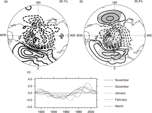
As has been confirmed earlier, the COWL-like pattern is dominant in multi-decadal changes in the wintertime circulation, in which interannual variability associated, for example, with AO and AIS are embedded. The interannual variability has been extracted locally in monthly SLP anomaly fields, by removing the first four harmonics from the original centennial anomaly time series at every grid point. Unlike its counterpart for the multi-decadal anomalies, EOF1 of the interannual SLP anomalies thus constructed (Fig. 1b) resembles the ‘pure’ AO pattern with a high degree of axial symmetry, featuring in-phase SLP variability between the midlatitude Atlantic and Pacific. The corresponding PC1 time series (not shown) indicate that the AO-associated interannual variability is incoherent from one calendar month to another. In recognition of the fact that Fig. 1a and 1b represent SLP anomaly patterns that correspond to a unit standard deviation of the PC1 time series, we observe that the amplitude of the AO pattern in Fig. 1b tends to be three times larger than that of the COWL-like pattern in Fig. 1a, thus confirming the predominance of the former variability over the latter. We should point out that the conclusions of this paper on the year-to-year variability are qualitatively unchanged if the first four harmonics are not removed from the original monthly anomalies.

As in Nakamura and Honda (2002), anomalous intensities of the AIS were evaluated from monthly SLP anomalies averaged within the respective domains of (32°–54°N, 162°E–134°W) and (58°–70°N, 46°–10°W), as indicated in Fig. 1b with heavy shading. These two domains contain the climatological centres of those semi-permanent low-pressure systems, which are in the vicinities of local maxima of the interannual SLP variance (not shown). It should be pointed out that our results shown below are qualitatively insensitive to slight changes in the domain definitions. The AIS index was then defined as the correlation coefficient between the normalised anomalous intensities of the AIS over a given time period. In order to discuss the multi-decadal modulation of AIS, the index has been calculated for every 25 winters centred at every year between 1922 and 1997.

The method for identifying and classifying an AO event is almost identical to that used by Shi and Bueh (2012). As in our evaluation of the AIS index mentioned earlier, the identification of AO events was performed separately for the individual 25-yr periods. Over a given 25-yr period, the monthly AO index was defined as PC1 of SLP variability over the entire extratropical Northern Hemisphere poleward of 20°N. Any month for which the absolute value of the AO index exceeds 0.8 standard deviation (σ) is regarded as a ‘potential AO event’. Bearing it in mind that SLP anomalies observed in a particular month with a large value of the AO index do not necessarily show a canonical AO structure with a high degree of axial symmetry (Shi and Bueh, 2012), we need to classify these events further. For this purpose, the anomalous intensities of the three centres of action of AO were first defined as area-weighted averages of the monthly SLP anomalies over the Arctic (60–90°N), North Pacific (32°–54°N, 162°E–134°W) and Euro-Atlantic (30°–50°N, 46°W–20°E) domains, which are shown in Fig. 1b with stippling. For simplicity, the Aleutian Low and North Pacific domains are designated as the same geographical area. All the potential AO events identified above were then categorised into the following two types: ‘pure AO events’ and ‘remainder’ events. Consistently with the conventional AO pattern (Thompson and Wallace, 1998, 2000; Fig. 1b), an event of the pure AO is identified (1) if monthly SLP anomalies averaged separately over the Aleutian and Euro-Atlantic domains have the same sign while a SLP anomaly averaged over the Arctic domain has the opposite sign, and (2) if each of their absolute values exceeds 0.4σ. Other choices for the threshold for (2), such as 0.3σ or 0.5σ, do not qualitatively alter the conclusion of this study.

3. Results

Following Honda et al., (2005a), we calculated AIS index separately for the individual calendar months and for the individual 25-yr periods centred at every year between 1922 and 1997. As evident in Fig. 2a, significant AIS signal was observed in December–January in the 1930s through the 1950s. After an inactive AIS period, significant AIS signal emerged again in the mid-1970s through the mid-1990s, but its peak time was shifted into January–February. Though based on a different data set, these results are consistent with the finding by Honda et al. (2005a). Our analysis has identified another period of active AIS after the mid-1990s, in which the peak time of the AIS signature is in January as was in the 1930s through the 1950s. Figure 2b shows the intensity of year-to-year variability of the Aleutian Low for every 25-yr period, defined as its standard deviation. Obviously, the three periods of active AIS (Fig. 2a) correspond well to the periods of particularly enhanced variability of the Aleutian Low, which seems consistent with the AIS formation that is triggered by the anomalous Aleutian Low (Honda et al., 2001, 2005b).

Fig. 2 November–March statistics for a 25-yr moving period centred at a given year on the abscissa. (a) AIS index (see text for further detail). Contour intervals are 0.2. Light, moderate and heavy shading indicate significance at the 90%, 95% and 99% confidence levels, respectively, based on one-tailed t-test. (b) AL variability (hPa) defined by 25-yr standard deviation of SLP anomalies averaged over the AL domain (32°–54°N, 162°E–134°W). (c) Percentage of ‘pure AO events’ among all the ‘potential AO events’ with large AO index values regardless of their signs. (d) AL anomaly (hPa) defined by area-averaged SLP anomalies in EOF1 over the AL domain. Dotted domains bounded by solid black lines indicate periods in which EOF1 is not well separated from other EOFs.

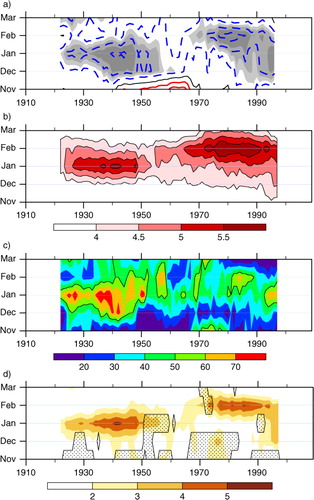
Figure 2c shows the percentage of the ‘pure AO events’ among all the potential AO events identified for every 25-yr period regardless of their signs. In agreement with Shi and Bueh (2012), not all the ‘potential AO events’ observed can be regarded as ‘pure AO events’. This is also the case even when the threshold of the AO index values for identifying a ‘potential AO event’ is raised to 1.5σ. Figure 2c indicates that those active-AIS periods (Fig. 2a) correspond, though not perfectly, to the fractional maxima of pure AO events relative to the potential AO events, for example, in January in the 1930s through 1950s and in the 1990s as well as in February in the mid-1970s through the 1980s. It is thus suggested that the AIS formation tends to accompany the occurrence of ‘pure AO events’. This seems consistent with Honda and Nakamura (2001), who showed that the northern fringe of the Aleutian Low and the southern fringe of the Icelandic Low are almost at the same latitude and their seesaw relationship (AIS) changes zonal winds coherently over the North Atlantic and Pacific.

In recognition of the dependence of a degree of axial symmetry of the AO structure upon the strength of the Aleutian Low anomaly within EOF1 of SLP anomalies (Deser, 2000; Ambaum et al., 2001), we examine multi-decadal modulations in the strength of the Aleutian Low anomaly in relation to those in the AIS signature. For this purpose, EOF1 of SLP anomalies was defined for each of the 25-yr periods centred at individual years separately for individual calendar months. For a given calendar month, EOF1 structure was determined by linearly regressing SLP anomalies over a given 25-yr period upon the corresponding normalised PC1. The polarities of EOF1 and PC1 were determined in such a manner that positive values of PC1 correspond to the positive phase of the pure AO characterised by negative SLP anomalies over the polar region. The Aleutian Low anomaly was then defined as the area-averaged SLP anomaly within the Aleutian domain (see Section 2) represented in EOF1 for a given 25-yr period.

Over the past 100 yr, the intensity of the anomalous Aleutian Low signature extracted in EOF1 (Fig. 2d) corresponds well to the AIS signal in Fig. 2a. Specifically, the Aleutian Low anomaly extracted in EOF1 tended to be particularly strong in the 1930s through the 1940s and then in the 1970s through the 1980s, whereas their peak month was changed from January to February from the former period to the latter. During the transition period in the 1960s, in contrast, the AIS signal was diminished and the Aleutian Low anomaly in EOF1 was also weak even in midwinter. In the latest period, the Aleutian Low anomaly still tends to be strong both in January and February. These multi-decadal modulations in the Aleutian Low signature in EOF1 are in good agreement with those of the year-to-year variability of the Aleutian Low shown in Fig. 2b and AIS index in Fig. 2a. These results suggest the particular importance of the Aleutian Low variability for the well-defined AIS signal and for the formation of AO-like axially symmetric structure. The most important feature shown in Fig. 2 is that the consistency among the four indices with respect to calendar months for which the indices maximise during the three multi-decadal periods. As shown in Honda et al. (2001, 2005a), the AIS signature exhibits distinct evolution within the season, reflecting Rossby-wave teleconnection from the anomalous Aleutian Low into the North Atlantic. The particular consistency supports our hypothesis that the AIS formation triggered by the anomalous Aleutian Low leads to the formation of the ‘pure AO’ pattern with a high degree of axial symmetry.

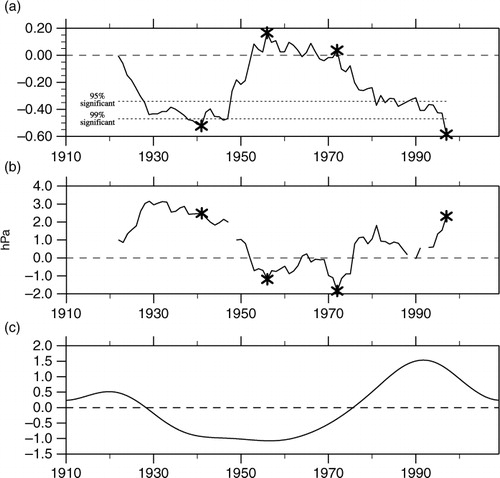
As observed in Fig. 2a, significant AIS signal tends to emerge in December and persist into February or March. Thus, we construct winter-mean anomalies by averaging monthly SLP anomalies from December to March, to explore the relationship between AIS signal and AO pattern and its multi-decadal modulations in a simpler manner. In a manner consistent with Fig. 2a, the AIS signal (Fig. 3a), whose strength is measured as the anti-correlation in intensity between the AIS over 25 winters, was pronounced also in the winter-mean anomalies for the period around the 1930s and 1940s, before diminished in the following period around the 1950s through the mid-1970s. Figure 3a further indicates that the AIS signal strengthened again in the late-1970s, which was most evident in late winter (Fig. 2a). After the mid-1990s, the AIS signal became even more enhanced, especially in the 25-yr period centred at 1997. Figure 3b shows the time series of the corresponding Aleutian Low anomaly extracted in EOF1 of winter-mean SLP anomalies.

Fig. 3 (a) and (b): As in Fig. 2a and 2d, respectively, but based on winter-mean (December—March) anomalies. In (b), the AL anomaly is not plotted when the corresponding EOF1 is not separated well from other EOFs. Asterisks denote the four 25-yr periods centred at 1941, 1956, 1972 and 1997, for each of which EOF1 of winter-mean SLP anomalies is shown in Fig. 4. (c) PC time series for EOF1 of multi-decadal SLP anomalies constructed only from the first four harmonics over the 1910–2009 period (i.e., with periods of 25 yr or longer). The PC values have been averaged within individual winter seasons before plotted. The corresponding SLP anomaly pattern is given in Fig. 1a, whose polarity corresponds to positive PC values.

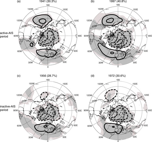
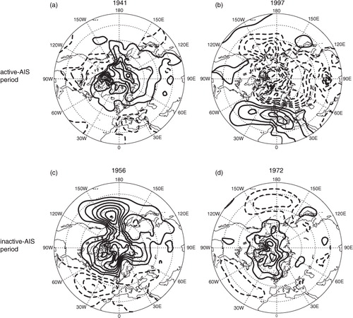
For the purpose of highlighting the multi-decadal modulations in the axial symmetry of winter-mean SLP anomalies extracted in their interannual EOF1, we specify two 25-yr periods centred at 1941 and 1997 to typify the active-AIS periods and two others at 1956 and 1972 to typify the inactive-AIS period. For each of these four 25-yr periods, whose central years are marked with asterisks in Fig. 3b, EOF1 of winter-mean SLP anomalies is shown in Fig. 4. The anomaly pattern in each of the panels in Fig. 4 corresponds to the positive phase of AO, and the signs of the anomalies have to be reversed for its negative phase. In interannual EOF1 for the active-AIS periods (Fig. 4a, b), positive SLP anomalies evident in the Aleutian region and the midlatitude Atlantic both act to enhance the axial symmetry of EOF1, typifying the ‘pure AO pattern’. In the corresponding EOF1 for the inactive-AIS period (Fig. 4c, d), in contrast, the axial symmetry of EOF1 is apparently reduced with negative SLP anomalies in the Aleutian region and positive anomalies in the midlatitude Atlantic. Unlike the ‘pure AO pattern’ (e.g., Fig. 1b), EOF1 of interannual SLP variability for the inactive periods represent a meridional pressure seesaw between the Atlantic and Arctic. This anomaly pattern thus bears some resemblance to the COWL pattern, which is also dominant in multi-decadal SLP variability (Fig. 1a).

Fig. 4 EOF1 of winter-mean SLP anomalies over the extratropical Northern Hemisphere (poleward of 20°N) defined for four 25-yr periods, whose central years are labelled in the panels and denoted with asterisks in Fig. 3. The fraction (%) of the SLP variance explained by EOF1 over each of the periods is shown in brackets. Contour interval is 1.5 hPa, and zero lines are omitted. The polarity corresponds to the positive phase of AO. Light and heavy shading indicates the anomalies significant at the 95% and 99% confidence levels, respectively. Each of the periods, EOF1 is well separated from other EOFs.

The results thus far are based on the statistics for a 25-winter sliding window. We have confirmed that changing the length of the window into 15 or 30 winters yields no qualitative changes in our statistics. Qualitatively the same results have also been obtained by using other reanalysis products, including the NCEP/NCAR Reanalysis (Kalnay et al., 1996) for the period 1948–2011 and the ERA Interim reanalysis data (Dee et al., 2011) for the period 1979–2011 (not shown).

4. Summary and discussion

Through an EOF analysis applied to 100-yr monthly SLP anomalies over the wintertime extratropical Northern Hemisphere taken from the 20th Century Reanalysis, we have found that the interannual variability of the Aleutian Low has been modulated on multi-decadal scales in concert with the AIS signal, whose multi-decadal modulations have also been in concert with those in the degree of axial symmetry of the AO pattern defined as EOF1 of interannual SLP variability. Our analysis has also revealed that ‘pure AO events’, characterised by axially symmetric structure of SLP anomalies, are more likely to occur during decadal periods in which AIS formation through inter-basin Rossby-wave teleconnection is active in association with the enhanced variability of the Aleutian Low. Our finding is consistent with both the NAM-augmented PNA perspective (Wallace and Thompson, 2002) and the NAO-PNA perspective (Ambaum et al., 2001) on the axial symmetry of AO.

We should point out that, if AO purely represents a dynamical mode, we cannot rule out the possibility that the pure AO pattern may trigger the AIS formation. Moreover, mechanisms that caused the multi-decadal modulations in interannual AIS signal and the axial symmetry of the AO pattern over the last century have not been clarified. As shown in Fig. 1a, the COWL-like pattern accounted for the largest fraction (26%) of the hemispheric multi-decadal variance. This variance includes the contribution from multi-decadal changes in the background state in which year-to-year variability associated with AO and/or AIS is embedded. The time series of the multi-decadal COWL-like pattern (Figs. 1c and 3c) indicates that during the last 100-yr period, the multi-decadal pattern was in the negative phase in the 1930s through the 1960s and then turned into the positive phase since the 1980s, representing a recent deepening trend of the Icelandic Low. However, these time series are not overall coherent with the corresponding time series that represents multi-decadal modulations of the AO and/or AIS (Figs. 2 and 3a, b). This incoherency is not necessarily surprising, since the multi-decadal COWL-like pattern in Fig. 1a exhibits only a weak anomaly over the North Pacific, where multi-decadal modulations of the Aleutian Low have been occurring with their potential influence on the axial symmetry of the AO pattern. The COWL-like pattern in Fig. 1a accounts only for 26% of the hemispheric multi-decadal variance, and another anomaly pattern might therefore be responsible for the multi-decadal modulations in the AIS signature. Figure 5 shows the winter-mean SLP anomalies averaged over each of the four 25-yr periods as deviations from the 100-yr climatological mean. Although the 25-yr anomaly patterns for the periods centred at 1956 and 1997 (Fig. 5b, c) are indeed similar to the COWL-like pattern in Fig. 1a, the corresponding anomaly patterns for the periods centred at 1956 and 1997 are not (Fig. 5a, d). Further study based on longer data sets and centennial integrations with realistic global climate models is required to deepen our understanding of the mechanisms through which the multi-decadal changes in the background state, including the contribution from the COWL-like pattern, have modulated the interannual AO pattern and of how the long-term modulations of the Aleutian Low variability and associated AIS formation could influence the hemispheric-scale variability. In particular, it is important to explore the mechanisms that modulated the interannual variability of the Aleutian Low on multi-decadal scales, which may possibly occur in conjunction with the corresponding modulations in SST variability (Miyasaka et al., 2014).

Fig. 5 Same as in Fig. 4, but for the 25-yr mean SLP anomalies. Contour interval is 0.4 hPa. Zero lines are omitted.

5. Acknowledgements

The authors are very grateful to the two anonymous reviewers for their sound criticism and useful suggestions that have led to substantial improvement of this paper. The authors are also grateful to K. Nishii and T. Miyasaka for their helpful comments. NS is supported jointly by the Chinese Natural Science Foundation (41105042 and 41375064) and the Priority Academic Program Development of Jiangsu Higher Education Institutions (PAPD). HN is supported in part by the Japanese Ministry of Environment through the Environment Research and Technology Development Fund A1201 and by the Japan Society of Promotion of Science through a Grant-in-Aid for Scientific Research in Innovative Areas 2205. The NCAR Command Language (NCL) was used for the calculation and drawing the plots.

Notes

¹It should be noted that the contour interval in Fig. 1b is three times greater than in Fig. 1a.

References

- Ambaum M. H. P. , Hoskins B. J. , Stephenson D. B . Arctic Oscillation or North Atlantic Oscillation?. J. Clim. 2001; 14: 3495–3507.
- Bjerknes J . A possible response of the atmospheric Hadley circulation to equatorial anomalies of ocean temperature. Tellus. 1966; 18: 820–829.
- Compo G. P. , Whitaker J. S. , Sardeshmukh P. D. , Matsui N. , Allan R. J. , co-authors . The twentieth century reanalysis project. Quart. J. Roy. Meteor. Soc. 2011; 137: 1–28.
- Dee D. P. , Uppala S. M. , Simmons A. J. , Berrisford P. , Poli P. , co-authors . The ERA-Interim reanalysis: configuration and performance of the data assimilation system. Quart. J. Roy. Meteor. Soc. 2011; 137: 553–597.
- Deser C . On the teleconnectivity of the “Arctic Oscillation”. Geophys. Res. Lett. 2000; 27: 779–782.
- Hannachi A. , Jolliffe I. T. , Stephenson D. B . Empirical orthogonal functions and related techniques in atmospheric science: a review. Int. J. Climatology. 2007; 27: 1119–1152.
- Hannachi A. , Jolliffe I. T. , Stephenson D. B. , Trendafilov N . In search of simple structures in climate: simplifying EOFs?. Int. J. Climatology. 2006; 266: 7–28.
- Honda M. , Nakamura H . Interannual seesaw between the Aleutian and Icelandic lows. Part II: its significance in the interannual variability over the wintertime Northern Hemisphere. J. Clim. 2001; 14: 4512–4529.
- Honda M. , Nakamura H. , Ukita J. , Kousaka I. , Takeuchi K . Interannual seesaw between the Aleutian and Icelandic lows. Part I: seasonal dependence and life cycle. J. Clim. 2001; 14: 1029–1042.
- Honda M. , Kushnir Y. , Nakamura H. , Yamane S. , Zebiak S. E . Formation, mechanisms, and predictability of the Aleutian-Icelandic low seesaw in ensemble AGCM simulations. J. Clim. 2005b; 18: 1423–1434.
- Honda M. , Yamane S. , Nakamura H . Impacts of the Aleutian–Icelandic Low seesaw on surface climate during the twentieth century. J. Clim. 2005a; 18: 2793–2802.
- Jolliffe I. T . Principal Component Analysis.
- Kalnay E. , Kanamitsu M. , Kistler R. , Collins W. , Deaven D. , co-authors . The NCEP/NCAR 40-year reanalysis project. Bull. Am. Meteorol. Soc. 1996; 77: 437–470.
- Kodera K. , Coughlin K . Apparent vertical propagation of the NAM index due to an embedded wave structure. J. Meteor. Soc. Japan. 2007; 85: 927–931.
- Kodera K. , Kuroda Y . Tropospheric and stratospheric aspects of the Arctic Oscillation. Geophys. Res. Lett. 2000; 27: 3349–3352.
- Kuroda Y . On the influence of the meridional circulation and surface pressure change on the Arctic Oscillation. J. Geophys. Res. 2005; 110: D21107.
- Miyasaka T. , Nakamura H. , Taguchi B. , Nonaka M . Multi-decadal modulations in low-frequency climate variability in the wintertime North Pacific since 1950. Geophys. Res. Lett. 2014; 41: 2948–2955.
- Nakamura H. , Honda M . Interannual seesaw between the Aleutian and Icelandic Lows Part III: its influence upon the stratospheric variability. J. Meteor. Soc. Japan. 2002; 80: 1051–1067.
- North G. R. , Bell T. L. , Cahalan R. F. , Moeng F. J . Sampling errors in the estimation of empirical orthogonal functions. Mon. Wea. Rev. 1982; 110: 699–706.
- Rogers J. C. , Van Loon H . The seesaw in winter temperatures between Greenland and Northern Europe. Part II: some oceanic and atmospheric effects in middle and high latitudes. Mon. Wea. Rev. 1979; 107: 509–519.
- Shi N. , Bueh C . The COWL pattern identified with a large AO index and its impact on annular surface temperature anomalies. Acta Meteorologica Sinica. 2012; 26: 410–419.
- Thompson D. W. J. , Wallace J. M . The Arctic Oscillation signature in the wintertime geopotential height and temperature fields. Geophys. Res. Lett. 1998; 25: 1297–1300.
- Thompson D. W. J. , Wallace J. M . Annular modes in the extratropical circulation. Part I: month-to-month variability. J. Clim. 2000; 13: 1000–1016.
- Thompson D. W. J. , Wallace J. M. , Hegerl G. C . Annular modes in the extratropical circulation. Part II: trends. J. Clim. 2000; 13: 1018–1036.
- van Loon H. , Rogers J. C . The seesaw in winter temperatures between Greenland and northern Europe. Part I: general description. Mon. Wea. Rev. 1978; 106: 296–310.
- Walker G. T. , Bliss E. W . World weather V. Mem. R. Meteorol. Soc. 1932; 4: 53–84.
- Wallace J. , Thompson D . The Pacific center of action of the Northern Hemisphere annular mode: real or artifact?. J. Clim. 2002; 15: 1987–1991.
- Wallace J. M. , Gutzler D. S . Teleconnections in the geopotential height field during the Northern Hemisphere winter. Mon. Wea. Rev. 1981; 109: 784–812.
- Wallace J. M. , Zhang Y. , Bajuk L . Interpretation of interdecadal trends in Northern Hemisphere surface air temperature. J. Clim. 1996; 9: 249–259.
- Wallace J. M. , Zhang Y. , Renwick J. A . Dynamic contribution to hemispheric mean temperature trends. Science. 1995; 270: 780–783.
- Wu Q. , Straus D. M . AO, COWL, and observed climate trends. J. Clim. 2004; 17: 2139–2156.
- Zhang X. , Sorteberg A. , Zhang J. , Gerdes R. , Comiso J. C . Recent radical shifts of atmospheric circulation and rapid changes in Arctic climate system. Geophys. Res. Lett. 2008; 35: L22701.
- Zhao H. , Moore G. W. K . Timescale dependency of spatial patterns in the variability of the Northern Hemisphere winter SLP field. Geophys. Res. Lett. 2006; 33: L13710.