Evaluation of conditional non-linear optimal perturbation obtained by an ensemble-based approach using the Lorenz-63 model

Abstract

The authors propose to implement conditional non-linear optimal perturbation related to model parameters (CNOP-P) through an ensemble-based approach. The approach was first used in our earlier study and is improved to be suitable for calculating CNOP-P. Idealised experiments using the Lorenz-63 model are conducted to evaluate the performance of the improved ensemble-based approach. The results show that the maximum prediction error after optimisation has been multiplied manifold compared with the initial-guess prediction error, and is extremely close to, or greater than, the maximum value of the exhaustive attack method (a million random samples). The calculation of CNOP-P by the ensemble-based approach is capable of maintaining a high accuracy over a long prediction time under different constraints and initial conditions. Further, the CNOP-P obtained by the approach is applied to sensitivity analysis of the Lorenz-63 model. The sensitivity analysis indicates that when the prediction time is set to 0.2 time units, the Lorenz-63 model becomes extremely insensitive to one parameter, which leaves the other two parameters to affect the uncertainty of the model. Finally, a serial of parameter estimation experiments are performed to verify sensitivity analysis. It is found that when the three parameters are estimated simultaneously, the insensitive parameter is estimated much worse, but the Lorenz-63 model can still generate a very good simulation thanks to the relatively accurate values of the other two parameters. When only two sensitive parameters are estimated simultaneously and the insensitive parameter is left to be non-optimised, the outcome is better than the case when the three parameters are estimated simultaneously. With the increase of prediction time and observation, however, the model sensitivity to the insensitive parameter increases accordingly and the insensitive parameter can also be estimated successfully.

• CNOP-P
• parameter sensitivity
• parameter estimation

1. Introduction

Model parameters can greatly impact model outputs (Hamby, 1994). Since there are many empirical parameters used to parameterise physical processes, some of them may cause significant uncertainties in weather and climate predictions (Lu and Hsieh, 1998; Mu et al., 2002). Effects of different parameters on model prediction vary (Hall et al., 1982; Hall, 1986). The ability to judge which parameters are more important is beneficial for reducing uncertainties in model prediction. Parameter sensitivity analysis provides an efficient way to estimate relative sensitivity of model parameters. As Navon (1998) suggested, relative sensitivity could serve as a guide to identify most important parameters whose changes impact most relevant responses in the atmospheric or ocean models.

Generally, there are two kinds of parameter sensitivity analysis methods for atmospheric and ocean models, namely, the one-at-a-time method (Hamby, 1994) and the adjoint method (Hall et al., 1982). The one-at-a-time method considers each model parameter and uses different values of this parameter to investigate the effect of its uncertainties on weather and climate simulations (Chu, 1999; Liu, 2002; Orrell, 2003). However, in realistic predictions, multiple model parameters may simultaneously have uncertainties (Mu et al., 2010). The adjoint method is the commonest sensitivity analysis method, which was first presented by Hall et al. (1982). Subsequently, the method was applied widely in parameter sensitivity analysis, especially in recent years (Zou et al., 1993; Lea et al., 2000; Moolenaar and Selten, 2004; Janisková and Morcrette, 2005; Daescu and Todling, 2010; Dacian and Navon, 2013). For the adjoint method, it not only has limitations in requiring the adjoint model but also does not give information on the physical effects of second- and higher-order derivatives of model results with respect to parameters. Thus, the adjoint method does not consider the non-linear interaction between parameters nor the non-linear interaction between parameters and model results. There is, hence, a need to develop a new method.

Mu et al. (2003) introduced the concept of conditional non-linear optimal perturbation (CNOP), which described the initial perturbation that had the largest non-linear evolution at prediction time and whose non-linear evolution described the maximum evolution of initial perturbations at prediction time (Mu and Zhang, 2006). The CNOP method was used in many studies (Duan et al., 2004, 2009; Mu et al., 2004, 2007, 2009). Furthermore, Mu et al. (2010) extended the CNOP method to search for optimal model parameter perturbations (called CNOP-P), which caused the largest departure from a given reference state at a prediction time with physical constraints. Sun and Mu (2011) applied the CNOP-P method to discuss the impact of climate change on a grassland ecosystem. Duan and Zhang (2010) and Yu and Mu (2012) used the CNOP-P method, respectively, in a theoretical model and an intermediate complexity model, to investigate whether model parameter errors could cause a significant spring predictability barrier for El Niño events or not.

As Mu et al. (2010) pointed out, during the maximisation process to obtain CNOP-P, one had to integrate the adjoint model to compute the gradient of the cost function, which limited its broad applications in various complicated models that did not have an existing adjoint. To ameliorate this limitation, Wang and Tan (2010) proposed an ensemble-based approach to solve CNOP; their idealised numerical experiments showed a good equivalence between the ensemble-based method and adjoint-based method proposed by Mu et al. (2003). Based on Wang and Tan (2010), we aim to improve the approach and make it suitable for calculating CNOP-P in this study. Then we provide an extensive evaluation for the CNOP-P obtained by the ensemble-based approach using the Lorenz-63 model (Lorenz, 1963).

In the next section, we describe the methodology of the ensemble-based approach to obtain CNOP-P. Experimental design and results using the Lorenz-63 model are presented in Section 3. Parameter sensitivity analysis by the CNOP-P method is shown in Section 4. Summary and discussion are given in Section 5.

2. Ensemble-based approach for CNOP-P

Let M _τ(p) be the propagator of the non-linear prediction model M from t=0 (the initial time) to t=τ (the prediction time) with the parameter vector p. Let U(t) be the time-dependent model state that is a solution to the non-linear prediction model U(t) = M _t (p _b )(U ₀), where U ₀ is the initial value of U.

Assuming that a parameter perturbation p′ be superposed on the background parameter p _b , the corresponding prediction increment y′ satisfies the following non-linear relationship with p′:1

where y=M _τ(p)(U ₀) is a prediction from 0 to τ generated by the non-linear model M with p as the parameter vector. Here, p _b , p′ and p are all m _p -dimensional column vectors, while y′ and y are m _y -dimensional column vectors.

For a chosen norm , a parameter perturbation is called CNOP-P if and only if2

where is the cost function that attains its maximum value when the corresponding parameter perturbation equals to CNOP-P, and is the constraint of parameter perturbation defined by the norm . More detailed definition of CNOP-P can be found in Mu et al. (2010), in which the CNOP-P was obtained using the adjoint model. Here, we elaborate the ensemble-based approach to obtain CNOP-P as follows: a certain amount of parameter perturbation (p′) is employed to create the corresponding prediction increment (y′), a series of orthogonal bases of parameter perturbations are found by the singular value decomposition (SVD) technique, an approximate tangent relationship model between p′ and y′ is established to estimate the gradient of the cost function during the iteration of optimisation process, and the non-linear prediction model is used to obtain the cost function value during the iteration to guarantee the constrained parameter perturbation's non-linear influence on model prediction.

Choosing n parameter perturbation samples (), the corresponding prediction increment samples () can be obtained by3

Denote the parameter perturbation sample matrix as P and the corresponding prediction increment sample matrix as Y, that is,4

If all the chosen parameter perturbations are small enough when compared with p _b , a tangent linear relationship between and is approximately true according to eq. (3):5

where M′ is the tangent linear model of M.

Denote the SVD of parameter perturbation sample matrix P by6

where A _p is an m _p ×m _p matrix whose columns are the left singular vectors of P and the set of orthonormal eigenvectors of PP^T, B _p is an n×n matrix whose columns are the right singular vectors of P and the set of orthonormal eigenvectors of P^TP, and D _p is an m _p ×n diagonal matrix whose entries are the singular values of P.

Thereby, a parameter perturbation p′ can be projected onto the ensemble space with A _p as the projection matrix:7

where , and8

Accordingly, the prediction increment y′ can be projected onto the same ensemble space:9

where10

Using eq. (7) and based on the orthogonality of A _p , α can be expressed as11

Substituting α in eq. (9) with that in eq. (11), the following relationship between p′ and y′ can be established:12

Note that CNOP-P is related to a constrained maximisation problem. In order to adopt the existing optimisation algorithms that are often used to compute minimisation problems, the maximisation problem is transformed to a minimisation problem. In particular, we rewrite eq. (2) as follows:13

Its gradient with respect to the parameter perturbation vector p′ can be expressed as:14

We can derive from eq. (12). Then, we can obtain (A _y (A _p )⁻¹)^T=A _p (A _y )^T using the orthogonality of A _p , and derive:15

Finally, the gradient of can be formulated as:16

With this gradient information, eq. (13) can be minimised by optimisation algorithms, such as Spectral Projected Gradient 2 (SPG2; Birgin et al., 2001) adopted by this study. To guarantee the non-linearity of the optimal solution, the value of the cost function is calculated using the non-linear model in eq. (1). In this way, the adjoint model is no longer needed.

3. Experimental design and results

The model studied here is the Lorenz (1963) system, which is a famous non-linear dissipative dynamical system and often used to mimic atmospheric chaotic behavior, because there is an interesting qualitative similarity between the dynamics of the Lorenz-63 model and those of the large-scale atmospheric circulation (Palmer, 1993). The Lorenz-63 model has three differential equations, which are derived from the convection equations of Saltzman (1962) and whose solutions afford the simplest example of deterministic non-periodic flow. The three-component Lorenz equations are shown as follows:17

where model parameters are σ (the Prandtl number), r (a normalised Raleigh number) and b (a non-dimensional wavenumber). The state variables x, y and z measure the intensity of convective motion, the temperature difference between the ascending and descending currents, and the distortion of vertical temperature profile from linearity, respectively. In this paper, all the calculations are performed using a fourth-order Runge-Kutta method with a time step of 0.01 time units. In addition, the model prediction adopted is the time series prediction of the state variables x, y and z. That is to say, the cost function concerned can be expressed as follows:18

where n is the number of prediction time step and the background parameter vector is denoted by p _b =(σ, r, b)^T, which are set to (10, 28, 8/3)^T in this paper. The parameter perturbation vector is denoted by p′=(σ′, r′, b′)^T, and the standardised parameter perturbation vector is denoted by , which can be taken as relative sensitivity, with19

For a reference experiment, the standardised parameter perturbations satisfy the constraint:20

Since the standardised parameter perturbation is the primary focus of this study, we use ‘parameter perturbation’ instead of ‘standardised parameter perturbation’ from now on for simplicity.

For the reference experiment, the model initial conditions (x ₀, y ₀, z ₀) are fixed at (0.0, 1.0, 0.0) and the model prediction time is τ=0.2 time units (n=20 time steps). The setup for the reference experiment is marked as EXP-1.

3.1. The CNOP-Ps of Lorenz-63 model

First, the ensemble-based approach is used to obtain the CNOP-P of EXP-1. Considering that there are only three parameters in the model, the experiment is performed using an equal number of parameter perturbation samples. As the SPG2 algorithm adopted needs a starting point, we choose an arbitrary parameter perturbation (2.225209E−02, 0.0, 9.749279E−02), whose corresponding prediction error (or the square root of cost function) is 0.3424122, as the initial guess. Then, the optimisation process takes only two iterations, and the corresponding optimal parameter perturbation, namely, the CNOP-P is21

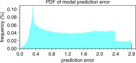
The result is encouraging since the prediction error is optimised to an amazing maximum value, namely, 2.794697. It increases by more than seven times comparing with the initial-guess prediction error. CNOP-P should cause the largest departure from a given reference state at a prediction time. So, is the optimal prediction error obtained by this approach large enough? To answer this question, the exhaustive attack method is employed, that is, a million random parameter perturbation samples are generated, which satisfy the following equality constraint:22

The same amount of the cost function values are also acquired through a million integrations of the Lorenz equations. The probability distribution function (PDF) of these prediction errors is shown in Fig. 1. The maximum and minimum value of prediction errors of the exhaustive attack method are 2.794695 and 0.01365796, respectively. The red bar in Fig. 1 corresponds to the probability of the prediction error that is greater than 2.794000. The probability is 0.0115% and thus very low. So, one can see that, if the prediction error with respect to the CNOP-P obtained by our ensemble-based approach belongs to such small probability event, the CNOP-P should be regarded as an effective result. As may be expected, the norm of the optimal parameter perturbation has attained the maximum value δ that the constraint permits, while the prediction error reaches its maximum value (2.794697), which is even greater than the maximum prediction error (2.794695) of the exhaustive attack method.

Fig. 1 The probability distribution function of prediction error when the model prediction time is set to 0.2 time units. The red bar represents the probability when the prediction errors are greater than 2.794000, while the maximum value of the prediction error of the exhaustive attack method is 2.794695.

3.2. Different prediction time steps

To evaluate the accuracy of the ensemble-based approach to obtain CNOP-P over an increasing model prediction time, we perform four experiments (marked as EXP-2) with the model prediction times set to τ=0.5, τ=1.0, τ=2.0 and τ=3.0 time units, respectively. The initial conditions, constraints and the number of samples used are the same as those used in EXP-1.

The experiment results are given in Table 1. The PDFs of the prediction errors are shown in Figs. 2a–d. The maximum prediction errors of the exhaustive attack method are 50.29931, 58.05915, 68.19436 and 87.88685 in the four experiments, respectively. All the red bars represent the probability of the prediction errors, which is less than but extremely close to the maximum value. The values of the probability are very small, so if the prediction errors obtained by the ensemble-based approach belong to these ranges, it can be approximately considered as the maximum value of the prediction error. From Table 1, one can easily see that the maximum prediction errors obtained by ensemble-based approach are 50.29834, 58.05844, 68.19016 and 87.75441, which are almost equal to the maximum values of the exhaustive attack method. The chaotic nature of the Lorenz-63 model, however, will limit the calculation of CNOP-P for longer prediction time. With the increase of prediction time, the maximum prediction error obtained by the ensemble-based approach decreases gradually compared to the maximum prediction error obtained by the exhaustive attack method.

Fig. 2 Same as Fig. 1, except that the model prediction time is set to (a) 0.5, (b) 1.0, (c) 2.0 and (d) 3.0 time units. The red bar represents the probability when the prediction errors are greater than (a) 50.25, (b) 58.00, (c) 68.10 and (d) 87.70, respectively.

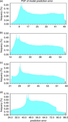
Table 1. CNOP-Ps with respect to an increasing model prediction time when the initial condition is fixed at (0.0, 1.0, 0.0)

Prediction time (time unit(s))	Maximum prediction error	Conditional non-linear optimal perturbation of parameter (σ′/σ, r′/r, b′/b)
0.5	50.29834	(5.166220 E − 02, 8.557348 E − 02, −2.863084 E − 03)
1.0	58.05844	(−4.357523 E − 02, −8.960319 E − 02, 8.512808 E − 03)
2.0	68.19016	(−3.291568 E − 02, −9.348051 E − 02, 1.333990 E − 02)
3.0	87.75441	(−2.160796 E − 02, −9.635826 E − 02, 1.575380 E − 02)

3.3. Different constraints

Here, another group of experiments with a varying critical constraint value δ are tested (marked as EXP-3), and δ is set to 0.01, 0.05 and 0.20, respectively. The initial conditions, model prediction time and the number of samples used are the same as those used in EXP-1.

The experiment results are given in Table 2, and the result of EXP-1 is also included for comparison. The PDFs of the prediction errors are shown in Figs. 3a–c. The maximum values of the exhaustive attack method are 0.2595068, 1.340676 and 6.082285 for the three δ values, respectively. All the red bars represent the probability of the prediction errors, which is almost equal to the maximum value. Table 2 shows the maximum prediction errors obtained by the ensemble-based approach are 0.2595067, 1.340678 and 6.082323, which are almost equal to, or even greater than, the maximum values of the exhaustive attack method. Although the three optimal parameter perturbations increase with the constraint, the first two parameter perturbations are always three orders of magnitude larger than the third. It means that the constraint has little influence on the pattern of CNOP-P.

Fig. 3 Same as Fig. 1, except that the critical constraint value is set to (a) 0.01, (b) 0.05 and (c) 0.20. The red bar represents the probability when the prediction errors are greater than (a) 0.2594, (b) 1.3400 and (c) 6.0800, respectively.

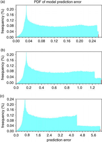
Table 2. CNOP-Ps with respect to a varying critical constraint value when the prediction time is set to 0.2 time units and the model initial condition is fixed at (0.0, 1.0, 0.0)

δ	Initial random prediction error	Maximum prediction error	Conditional non-linear optimal perturbation of parameter (CNOP-P)
0.01	3.420223 E − 02	0.2595067	(5.920789 E − 03, 8.058799 E − 03, −4.983945 E − 06)
0.05	0.1710982	1.340678	(2.960444 E − 02, 4.029363 E − 02, −2.490810 E − 05)
0.1	0.3424122	2.794697	(5.921009 E − 02, 8.058637 E − 02, −4.911502 E − 05)
0.2	0.6856751	6.082323	(1.184327 E − 01, 1.611635 E − 01, −9.726922 E − 05)

3.4. Different initial conditions

To evaluate the dependence of CNOP-P obtained by our approach on different initial conditions, three more experiments (marked as EXP-4) are conducted using three different initial conditions, namely, (1.0, 1.0, −1.0), (5.0, 5.0, 5.0) and (−10.0, −10.0, −10.0). The model prediction time, constraints and the number of samples used are the same as those used in EXP-1.

The experiment results are given in Table 3, and the PDFs of the prediction errors are shown in Figs. 4a–c. The maximum values of the prediction errors of the exhaustive attack method are 6.494038, 17.97263 and 20.19889 in the three cases, respectively. All the red bars represent the probability of the prediction errors, which are almost equal to the maximum value. Table 3 shows that the maximum prediction errors obtained by the ensemble-based approach are 6.493985, 17.96980 and 20.19837, which are almost equal to, or even greater than, the maximum values of the exhaustive attack method. We can see that the overall pattern of CNOP-P is consistent with that of EXP-1.

Fig. 4 Same as Fig. 1, except that the initial condition is set to (a) (1.0, 1.0, −1.0), (b) (5.0, 5.0, 5.0) and (c) (−10.0, −10.0, −10.0). The red bar represents the probability when the prediction errors are greater than (a) 6.49, (b) 17.95 and (c) 20.17, respectively.

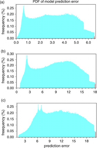
Table 3. CNOP-Ps with respect to different initial conditions when the prediction time is set to 0.2 time units

Initial conditions (x 0, y 0 , z 0)	Maximum prediction error	Conditional non-linear optimal perturbation of parameter (σ′/σ, r′/r, b′/b)
(1.0, 1.0, −1.0)	6.493985	(3.640889 E − 02, 9.313641 E − 02, −5.553383 E − 05)
(5.0, 5.0, 5.0)	17.96980	(2.122251 E − 02, 9.770686 E − 02, −1.724857 E − 03)
(−10.0, −10.0, −10.0)	20.19837	(2.615064 E − 02, 9.611105 E − 02, −8.877495 E − 03)

4. Parameter sensitivity analysis

As Mu et al. (2010) expected, CNOP-P can illuminate the most sensitive parameter perturbation and provide information on determining the sequence of sensitivity of model parameters. The standardised parameter perturbation (σ′/σ, r′/r, b′/b) could represent relative sensitivity of the corresponding parameter. Under the constraint of 2-norm of the parameter perturbation vector, the bigger the weighting is, the more sensitive the model prediction is to the parameter.

From eq. (21) in EXP-1, the model prediction is relatively more sensitive to the first two parameters (σ, r) and extremely insensitive to the third parameter (b) whose optimal perturbation weighting is three orders of magnitude smaller than those of the first two parameters. Then, let us pay attention to the CNOP-Ps under a varying model prediction time, which are shown in Table 1. We can see clearly in EXP-2 that with the increase of model prediction time from 0.5 to 3.0 time units, the value of relative sensitivity of the first parameter (σ) is getting smaller and that of the second parameter (r) is getting larger, while the third parameter (b) always keeps a low relative sensitivity. Further, the same analyses is done for EXP-3 and EXP-4, although in the experiments with different constraints and initial conditions, the first two parameters (σ, r) are always more important than the third parameter (b). Therefore, we could conclude that the first two parameters, especially the second parameter (r), are predominant on affecting the uncertainty of the Lorenz-63 model with τ=0.2 time units. With the increase of prediction time and the initial condition of EXP-1, the parameter (b) will become more important. The experiment results of the exhaustive attack method show that the optimal perturbation weighting of parameter (b) increases when the prediction time is increased from 3.0 to 6.0 time units (not shown). The same results are also obtained with different initial conditions for a longer time scale. For a long prediction time, but with the same experiment setup as those used in EXP-4, relative sensitivity of (σ) and (b) vary significantly with different initial conditions, while the second parameter (r) is always very important (not shown).

4.1. Estimation of the three parameters

To verify the CNOP-P obtained by the ensemble-based approach, the exhaustive attack method is employed in Section 3. The maximum prediction error and the relative parameter perturbation from the ensemble-based approach are consistent with those from the exhaustive attack method. Here, some idealised experiments of parameter estimation are performed to verify the sensitivity analysis by the CNOP-P method. Cacuci et al. (2013) discussed the issue of parameter identification and estimation and introduced some methods for parameter estimation, such as maximum likelihood (ML), maximum total variation and extended Kalman filter (EKF). Zhu and Navon (1999) applied the variational method using a full-physics adjoint of the FSU Global Spectral Model to recover three parameters as well as initial conditions. The parameter estimation method adopted here is an ensemble-based method originated from a data assimilation method (Wang et al., 2010; Liu et al., 2011), the procedure of which is similar to the approach in Section 2, except for a different cost function. More general cost functions can also be chosen (Cacuci et al., 2013), we express the cost function as follows:23

where y _obs is the observation vector, O is the observation error covariance matrix, which is a diagonal matrix only including the observation error variance, and the remaining variables are the same as the ones used in Section 2. The cost function here means distance between model prediction and observation. It attempts to find a suitable parameter perturbation under a certain constraint that is superimposed on the background parameter vector p _b and makes the cost function attain its minimum value.

Here, the model background prediction is denoted by24

and the model prediction increment y′ is still given by eq. (1). So, the cost function can be rewritten as follows:25

Accordingly, based on eqs. (15) and (25), the gradient of the cost function can be formulated as follows:26

In order to compare with the experiment results in Section 3, the basic setups of experiments, such as model prediction time and initial conditions are the same as those in EXP-1. Now, suppose that the true parameter vector p _t is as follows:27

Then, a set of synthetic observations are generated by a preliminary run of the Lorenz-63 model with the true parameter values in, for example (27). The cost function of parameter estimation experiments can be expressed as follows:28

where the background parameters are set to their default values:29

The cost function value corresponding to the parameter perturbation p′=(0, 0, 0)^T is 3.853652E + 01, which is the model prediction error before optimisation.

Two idealised experiments (marked as EXP-5) are performed with the critical constraint δ set to 0.30 and 0.40, respectively. In the first idealised experiment with δ=0.30, the cost function value is minimised to 2.717061E−04 when it converges (10 iterations), while the optimised parameter values are σ=11.49203, r=32.01417 and b=2.666177. In the second idealised experiment with δ=0.40, the cost function value is minimised to 6.330993E−04 after 20 iterations; it converges, and the optimised parameter values are σ = 11.48677, r=32.02354 and b=2.559506. We can see that in both experiments the parameters (σ, r) are estimated very closely to the true values, but the third parameter (b) is poorly estimated, with the optimised value much closer to the background parameter value.

These results are of great interest. The cost functions of both experiments are reduced drastically by almost 100% compared to the value of 3.853652E + 01 in the non-optimised situation, although the parameter (b) is much worse than the parameter value in the non-optimised situation. The Lorenz-63 model that contains relatively accurate values of the first two parameters and a very inaccurate value of the third parameter can still generate a very good simulation. This result indicates that the non-linear effects of σ and r on model prediction are the most crucial ones, while b exerts little influence on the cost function in this case. It is consistent with that of parameter sensitivity analysis from the CNOP-P method. Further, the insensitivity means that its non-linear effect on model prediction is very weak, and the cost function is less dependent on the insensitive parameter.

Observation data can improve not only model initial conditions but also model parameters. If the number of observations increases, how is the result under the same conditions as above? Next, we set time window to τ=2.0 time units, and the rest setups are the same as in the above experiments. With δ=0.40, the cost function before optimisation is 1.306569E + 04, while the optimised cost function is reduced to 7.704161E−10; the optimised parameter values are σ=11.50000, r=32.00000 and b=2.870000, which are equal to the true parameter values. Here, the true states are directly taken as observation. Annan and Hargreaves (2004) used Ensemble Kalman Filter (EnKF) to estimate the parameters of the Lorenz-63 model, and set the true and the background parameters the same; but the observation data was produced by adding random noise (with variance of 0.01) to the true states. Their results showed the three parameters would converge in about 200 EnKF sequential iterations. Here, the optimisation window is increased to 2.0 time units, namely, the number of observations is 200. Random noises are added to the observation with different variances of 0.01, 0.04 and 0.09, respectively, and the results are given in Table 4. All three parameters are close to the true values, including the third parameter, and observation errors have very small influences on the parameters estimated. This indicates that when there is sufficient observation, the optimised parameters can achieve a stable state that is close to the true state, which is consistent with the results of Annan and Hargreaves (2004).

Table 4. Optimised parameter values and corresponding optimised prediction errors with the prediction time set to 2.0 time units when random errors of different variances are added to the observations

Variance of observation errors	Optimised prediction error	Optimised parameter values (σ, r, b)	Number of iteration
0.01	3.258717	(11.59596, 31.88207, 2.862262)	13
0.04	4.851858	(11.59111, 31.74486, 2.867236)	13
0.09	7.159717	(11.57233, 31.63118, 2.867709)	13

The prediction error before optimisation is 114.3052.

From these experiments, we can see that the distance between the estimation of each parameter and the truth is proportional to the size of the observation errors when the number of observations is constant. Particularly, we can observe from Table 4 that with the gradual decrease of observation errors, the optimised cost function which represents the distance between the estimation of parameters and the truth decreases gradually. As Navon (1998) pointed out, a parameter is identifiable if and only if a unique solution of the optimisation problem exists and the solution depends continuously on the observations. Therefore, according to this criterion, our experiments, which show that both the optimised cost function and the estimation of parameters depend continuously on the size of observation errors, indicate that the parameters are identifiable.

4.2. Estimation of two parameters

Here, we use a new group of parameter estimation experiments to estimate only two parameters every time, namely, (σ, r), (σ, b) and (r, b), respectively. Except for this difference, the basic experiment setup is the same as that used in EXP-5 and the critical constraint δ is set to 0.30. The experiment results are shown in Table 5, and the results of EXP-5 are also included for comparison. When only the first two sensitive parameters (σ, r) are estimated simultaneously, the outcome is comparable to, or even better than, the case when all three parameters are estimated. When the other two parameter combinations (σ, b) and (r, b), including the insensitive parameter (b ), are estimated respectively, both parameters converge to the wrong values although the cost function values are still reduced to some extent. The reason for this poor outcome is that the optimisation of the two parameters (one of them is the insensitive parameter) may compensate for the error of the non-optimised important parameter when the cost function is minimised. Particularly, the cost function of the parameter combination (σ, b) is optimised to a worse value than that of the parameter combination (r, b), which may indicate the second parameter (r ) is more predominant than the first parameter (σ ). Therefore, the above results can further confirm that the model prediction is extremely insensitive to the third parameter (b) under the initial condition of EXP-1. This is also consistent with the conclusion of Cacuci et al. (2013) that correct estimations of important model parameters contribute significantly towards improving the estimation of the model state. Meanwhile, we could also conjecture that excessive insensitive parameters may cause parameter estimation to fail in view of the dimensionality and lack of enough sensitivity to the observation. So, it is expected that a good parameter estimation experiment should centre upon the most sensitive parameters and avoid the confusion by insensitive parameters.

Table 5. Optimised parameter values and corresponding optimised cost functions with the prediction time set to 0.2 time units and the critical constraint δ set to 0.30

Parameter estimated	Optimised cost function	Optimised parameter values (σ, r, b)	Number of iteration
(σ, r)	2.698106 E − 04	(11.49159, 32.01515, 8/3)	9
(σ, b)	3.031157 E + 00	(13.00000, 28, 2.665819)	1
(r, b)	5.351562 E − 01	(10, 23.85923, 3.362714)	18
(σ, r, b)	2.717061 E − 04	(11.49203, 32.01417, 2.666177)	10

The cost function and parameter values before optimisation are 3.853652 E + 01 and (10, 28, 8/3), respectively, while the true parameter values are (11.5, 32.0, 2.87).

5. Summary and discussion

In this paper, the ensemble-based approach is used to obtain the CNOP-Ps of the Lorenz-63 model. CNOP-P represents a type of model parameter perturbation which can cause the largest departure from a given reference state at a prediction time. A series of CNOP-P experiments show that the maximum prediction error after optimisation has been multiplied manifold compared with the initial-guess prediction error. In addition, the exhaustive attack method is employed to compare with our approach, that is, a million random parameter perturbation samples are generated satisfying the same constraint, and then the PDFs of a million prediction errors are computed. The results show that the prediction errors obtained by the ensemble-based approach are extremely close to, or even greater than, the maximum values of the exhaustive attack method. Three groups of experiments including different prediction time steps, different constraints and different initial conditions reveal that the CNOP-P obtained by the ensemble-based approach is capable of maintaining a high accuracy over a long prediction time under different constraints and initial conditions. In these idealised experiments, the number of perturbation samples is equal to that of model parameters, and we obtain very accurate results. For much more complicated models, such as weather and climate models, we may need to employ more samples in order to gain a relatively more accurate optimal parameter perturbation. It may be more practical for the ensemble-based approach to use more samples than the number of model parameters under consideration, which may provide more accurate gradient of the cost function and thus accelerate the convergence.

Based on the above experiments, a parameter sensitivity analysis is performed. The results show that model prediction is relatively more sensitive to the first two parameters (σ, r) and extremely insensitive to the third parameter (b), whose optimal perturbation weighting is three orders of magnitude smaller than those of the first two parameters. Moreover, with the increase of model prediction time from 0.5 to 3.0 time units, the relative sensitivity of the first parameter (σ) becomes smaller and that of the second parameter (r) becomes larger. Under the constraint of two-norm of the parameter perturbation vector, a more sensitive parameter will correspond to a larger weighting of optimal parameter perturbation. So, it can be concluded the first two parameters (σ, r), especially the second parameter (r), are predominant on affecting the uncertainty of the Lorenz-63 model with τ=0.2 time units. But for a longer time scale, relative sensitivity of parameters defined in our study may be influenced significantly by different initial conditions. The relative sensitivity of parameters that is independent of initial conditions would require further investigation.

The parameter sensitivity analysis is further verified through two groups of parameter estimation experiments, in which all three parameters or only two of the three parameters are estimated simultaneously, respectively. In the first case the parameters (σ, r) are estimated to be very close to the true values, but the third parameter (b) remains inaccurate. Although the parameter (b) is much worse than the parameter value in the non-optimised situation, the Lorenz-63 model that contains relatively accurate values of the first two parameters can still generate a very good simulation. In another case when only the first two sensitive parameters (σ, r) are estimated simultaneously, the result is comparable to and even better than the case when all three parameters are estimated. When the other two parameter combinations (σ, b) and (r, b), including the insensitive parameter (b), are estimated respectively, however, the result is not satisfactory. Therefore, the results of these two cases provide a consistent conclusion with the relative sensitivity analysis by the CNOP-P method that the non-linear effects of the first two parameters (σ, r) on model prediction are the most crucial ones while the third parameter (b) exerts little influence. In addition, the insensitive parameter is difficult to be estimated precisely, and may exert a negative influence on parameter estimation. It must be emphasised that these results are obtained at a short prediction time (τ=0.2 time units). With the increase of prediction time, the parameter (b) will become more sensitive and can also be estimated successfully.

We perform an analogous experiment with the optimisation window increased to 2.0 time units and different random noises added to the observations. The result shows that the optimised parameters obtained by our approach are close to the truth values, including the third parameter (b), which agrees with the results of Annan and Hargreaves (2004). Although parameter estimation is not the focus of this paper, we show that the ensemble-based method for parameter estimation is capable of simultaneously estimating all three model parameters.

It is worth discussing the possibility when the cost function attains its local maximum in a small neighbourhood of a point in the phase space, whose corresponding parameter perturbation is called local CNOP-P (Mu and Zhang, 2006). In this study, local CNOP-Ps of EXP-2 are given in Table 6. We can see that the direction of local CNOP-Ps is approximately opposite to that of global CNOP-Ps (see Table 1), while the prediction errors corresponding to local CNOP-Ps are a bit smaller than the global maximum values. So, relative sensitivity obtained by local CNOP-P may be equivalent to that by global CNOP-P, which indicates that local CNOP-P may be also very useful.

Table 6. Local CNOP-Ps with respect to an increasing model prediction time when the model initial condition is fixed at (0.0, 1.0, 0.0)

Prediction time (time unit(s))	Local maximum prediction error	Local conditional non-linear optimal perturbation of parameter (σ′/σ, r′/r, b′/b)
0.5	48.77164	(−5.727754 E − 02, −8.192971 E − 02, 2.608925 E − 03)
1.0	56.57906	(4.356946 E − 02, 8.968048 E − 02, −7.688598 E − 03)
2.0	67.49694	(3.075451 E − 02, 9.356575 E − 02, −1.730929 E − 02)
3.0	77.14283	(1.979255 E − 02, 9.762610 E − 02, −8.797674 E − 03)

So far, the CNOP-P method has only been tested in the Lorenz-63 model. Since the method is easy to implement, a natural next step is to test the method using a more realistic atmospheric model. In fact, an application in the Weather Research and Forecasting (WRF) model is on the way.

Acknowledgements

We acknowledge the Ministry of Science and Technology of China for funding the 973 Project (Grant No. 2010CB951604), the National Science and Technology Support Program (Grant No. 2012BAC22B02) and the National Natural Science Foundation of China (Grant No. 41105120).

References

- Annan J. D , Hargreaves J. C . Efficient parameter estimation for a highly chaotic system. Tellus A. 2004; 56: 520–526.
- Birgin E. G , Martinez J. M , Raydan M . Algorithm 813: SPG: software for convex-constrained optimization. ACM Trans. Math. Software. 2001; 27: 340–349.
- Cacuci D. G , Navon I M , Ionescu-Bujor M . Computational Methods for Data Evaluation and Assimilation.
- Chu, P. C. 1999. Two kinds of predictability in the Lorenz system. J. Atmos. Sci. 56, 1427–1432.
- Dacian N. D , Navon I. M , Farago I , Zlatev Z . Sensitivity analysis in nonlinear variational data assimilation: theoretical aspects and applications. Chapter 4 in the E-book: Advanced Numerical Methods for Complex Environmental Models: Needs and Availability. 2013; Oak Park, Illinois, USA: Bentham Science Publishers. 282–306.
- Daescu D. N , Todling R . Adjoint sensitivity of the model forecast to data assimilation system error covariance parameters. Q. J. Roy. Meteorol. Soc. 2010; 136: 2000–2012.
- Duan W , Liu X , Zhu K , Mu M . Exploring the initial errors that cause a significant “spring predictability barrier” for El Nino events. J. Geophys. Res. 2009; 114: C04022.
- Duan W , Mu M , Wang B . Conditional nonlinear optimal perturbation as the optimal precursors for El Nino-Southern Oscillation events. J. Geophys. Res. 2004; 109: D23105.
- Duan W , Zhang R . Is model parameter error related to a significant spring predictability barrier for El Niño events? Results from a theoretical model. Adv. Atmos. Sci. 2010; 27(5): 1003–1013.
- Hall M. C . Application of adjoint sensitivity theory to an atmospheric general circulation model. J. Atmos. Sci. 1986; 43: 2644–2651.
- Hall M. C , Cacuci D. G , Schlesinger M. E . Sensitivity analysis of a radiative-convective model by the adjoint method. J. Atmos. Sci. 1982; 39: 2038–2050.
- Hamby D. M . A review of techniques for parameter sensitivity analysis of environmental models. Environ. Monit. Assess. 1994; 32: 135–154.
- Janisková M , Morcrette J. J . Investigation of the sensitivity of the ECMWF radiation scheme to input parameters using the adjoint technique. Q. J. Roy. Meteorol. Soc. 2005; 131: 1975–1995.
- Lea D. J , Allen M. R , Haine T. W . Sensitivity analysis of the climate of a chaotic system. Tellus A. 2000; 52: 523–532.
- Liu J , Wang B , Xiao Q . An evaluation study of the DRP-4-DVar approach with the Lorenz-96 model. Tellus A. 2011; 63: 256–262.
- Liu Z. Y . A simple model study of ENSO suppression by external periodic forcing. J. Atmos. Sci. 2002; 15: 1088–1098.
- Lorenz E. N . Deterministic nonperiodic flow. J. Atmos. Sci. 1963; 20: 130–141.
- Lu J , Hsieh W. W . On determining initial conditions and parameters in a simple coupled atmosphere-ocean model by adjoint data assimilation. Tellus A. 1998; 50: 534–544.
- Moolenaar H. E , Selten F. M . Finding the effective parameter perturbations in atmospheric models: the LORENZ63 model as case study. Tellus A. 2004; 56: 47–55.
- Mu M , Duan W , Wang B . Conditional nonlinear optimal perturbation and its applications. Nonlinear Process. Geophys. 2003; 10: 493–501.
- Mu M , Duan W , Wang B . Season-dependent dynamics of nonlinear optimal error growth and El Nino-Southern Oscillation predictability in a theoretical model. J. Geophys. Res. 2007; 112: D10113.
- Mu M , Duan W , Wang J . Predictability problems in numerical weather and climate prediction. Adv. Atmos. Sci. 2002; 19: 191–205.
- Mu M , Duan W , Wang Q , Zhang R . An extension of conditional nonlinear optimal perturbation approach and its applications. Nonlinear Process. Geophys. 2010; 17: 211–220.
- Mu M , Sun L , Dijkstra H . The sensitivity and stability of the ocean's thermocline circulation to finite amplitude freshwater perturbations. J. Phys. Oceanogr. 2004; 34: 2305–2315.
- Mu M , Zhang Z . Conditional nonlinear optimal perturbation of a two-dimensional quasigeostrophic model. J. Atmos. Sci. 2006; 63: 1587–1604.
- Mu M , Zhou F , Wang H . A method for identifying the sensitive areas in targeted observations for tropical cyclone prediction: conditional nonlinear optimal perturbation. Mon. Wea. Rev. 2009; 137(5): 1623–1639.
- Navon I. M . Practical and theoretical aspects of adjoint parameter estimation and identifiability in meteorology and oceanography. Dynam. Atmos. Oceans. 1998; 27: 55–79.
- Orrell D . Model error and predictability over different timescales in the Lorenz'96 systems. J. Atmos. Sci. 2003; 60: 2219–2228.
- Palmer T. N . Extended-range atmospheric prediction and the Lorenz model. Bull. Am. Meteorol. Soc. 1993; 74: 49–65.
- Saltzman B . Finite amplitude free convection as an initial value problem-I. J. Atmos. Sci. 1962; 19: 329–341.
- Sun G , Mu M . Nonlinearly combined impacts of initial perturbation from human activities and parameter perturbation from climate change on the grassland ecosystem. Nonlinear Process. Geophys. 2011; 18: 883–893.
- Wang B , Liu J.-J , Wang S , Cheng W , Liu J , co-authors . An economical approach to four-dimensional variational data assimilation. Adv. Atmos. Sci. 2010; 27: 715–727.
- Wang B , Tan X . Conditional nonlinear optimal perturbations: adjoint-free calculation method and preliminary test. Mon. Wea. Rev. 2010; 138: 1043–1049.
- Yu Y , Mu M . Does model parameter error cause a significant “spring predictability barrier” for El Niño events in the Zebiak-Cane model?. J. Clim. 2012; 25: 1263–1277.
- Zhu Y , Navon I. M . Impact of parameter estimation on the performance of the FSU Global Spectral Model using its full physics adjoint. Mon. Wea. Rev. 1999; 127(7): 1497–1517.
- Zou X , Barcilon A , Navon I. M , Whitaker J , Cacuci D. G . An adjoint sensitivity study of blocking in a two-layer isentropic model. Mon. Wea. Rev. 1993; 121: 2833–2857.