Development of a wind gust model to estimate gust speeds and their return periods

Abstract

Spatially dense observations of gust speeds are necessary for various applications, but their availability is limited in space and time. This work presents an approach to help to overcome this problem. The main objective is the generation of synthetic wind gust velocities. With this aim, theoretical wind and gust distributions are estimated from 10 yr of hourly observations collected at 123 synoptic weather stations provided by the German Weather Service. As pre-processing, an exposure correction is applied on measurements of the mean wind velocity to reduce the influence of local urban and topographic effects. The wind gust model is built as a transfer function between distribution parameters of wind and gust velocities. The aim of this procedure is to estimate the parameters of gusts at stations where only wind speed data is available. These parameters can be used to generate synthetic gusts, which can improve the accuracy of return periods at test sites with a lack of observations. The second objective is to determine return periods much longer than the nominal length of the original time series by considering extreme value statistics. Estimates for both local maximum return periods and average return periods for single historical events are provided. The comparison of maximum and average return periods shows that even storms with short average return periods may lead to local wind gusts with return periods of several decades. Despite uncertainties caused by the short length of the observational records, the method leads to consistent results, enabling a wide range of possible applications.

• wind
• gusts
• extreme value statistics
• return periods
• windstorm
• observations

To access the supplementary material to this article, please see Supplementary files under Article Tools online.

1. Introduction

Wind gusts are short-time exceedances of mean wind speeds for a certain time range. As they often occur as concomitant phenomenon of severe windstorms or thunderstorms, they may lead to large socio-economic impacts and can affect large areas (Fink et al., 2009). Several studies have estimated the windstorm risk from a pan-European perspective under recent and/or future climate conditions (e.g. Della-Marta et al., 2009, 2010; Schwierz et al., 2010; Pinto et al., 2012). Wind energy estimates for recent decades and future projections have also been assessed (e.g. Barthelmie et al., 2008; Pryor and Barthelmie, 2010; Brayshaw et al., 2011; Hueging et al., 2013). In both cases, realistic estimates of observed wind gusts, their spatial and temporal variability and associated return periods are required. A common approach to estimate gusts is the use of numerical prediction models, which in turn should be validated by sufficiently long-term reference datasets of observations. For mean wind velocity, several datasets have been assembled by Gerth and Christoffer (1994) and Walter et al. (2006) for Germany or by Wieringa (1986) for the Netherlands. Such wind maps can also be divided into zones (Kasperski, 2002) as required, e.g. for wind energy prediction. For gust velocity, no comparable maps are available, as gust measurements are much sparser than wind measurements. The use of country-specific thresholds for reporting gusts (e.g. 12.5 ms⁻¹ for Germany) additionally intensifies the lack of observations.

There are several physical mechanisms that may lead to strong near-surface wind gusts, which are reflected in different parameterisations of numerical models. Three main approaches have been established. One is the consideration of a gust factor, defined as a fraction between gust and mean wind speed, which depends on the nearby environment (Wieringa, 1986; Verkaik, 2000). In Brasseur (2001), gusts are interpreted as downward momentum flux from the higher levels of the planetary boundary layer. Born et al. (2012) consider gusts as a sum of the mean wind speed and a turbulent part, explained through turbulent kinetic energy. All three approaches have in common that gusts are influenced by the large-scale wind, the roughness length and the atmospheric stability (or connected parameters). However, it is problematic that such parameters are not measured with standard instruments for wind or gust speed.

The influence of the roughness length is one of the main reasons for the spatial and temporal variability of wind and gust speeds. This parameter itself underlies seasonal variability and decadal trends (Wever, 2012). As wind and gust measurements are required to be representative for an area of several kilometres, the influence of the roughness length needs to be removed for comparisons of multiple measurement records. Usually, roughness length is derived through measurements of atmospheric fluxes in several heights, but for larger sets of observational records from different sites this approach is not applicable. Alternatively, there are two main approaches to derive roughness values through gustiness analysis, which were compared by Verkaik (2000). Both approaches require only periodical measurements of mean wind speed, mean wind direction and gust speed. The approach of Wieringa (1986, 1993) is less exact than the model of Beljaar (1987), but it is advantageous as it requires less information about the measuring chain.

To model the temporal variability of gusts, extreme value statistics (cf. Coles, 2001) can be used, since gusts are measured as a maximum of wind speed during a fixed time range. Commonly used approaches to estimate extreme gusts are the peak-over-threshold (POT) and the block maxima technique. The POT approach examines gust exceedances over a certain threshold, which can be modelled by a generalized Pareto-distribution characterized by a location, a scale and a shape parameter. The parameters themselves depend on the a priori threshold and the domain of attraction. This approach is analysed by several authors for extreme wind speed prediction (Brabson and Palutikof, 2000; Van de Vyver and Delcloo, 2011) and is usually used to estimate the probability of gusts above a warning level. Friedrichs et al. (2009) examined different methods for gust estimation above this level and pointed out that an extreme value approach performs much better than other approaches usually applied in model output statistics. Still, the POT approach suffers from high variations in the tail depending on the chosen threshold (An and Panley, 2005; Harris, 2005). For this reason, special estimators like the Zipf-estimator (Van de Vyver and Delcloo, 2011) are required.

The block maxima approach examines peaks over a certain time period or over a region. The distribution of these block maxima can be fitted by three types of probability functions: Gumbel, Fréchet or Weibull type. All three types are combined in the family of the Generalized Extreme Value distribution (GEV). This distribution is characterized by a location, a scale and a shape parameter. One disadvantage of the usage of this approach is the necessity of a large data basis, as only one value (the maximum), per subsample is used. In case of meteorological variables the approach is usually applied to annual maxima.

The main challenge of both approaches is the correct estimation of the parameters of the extreme value distribution. Van den Brink and Können (2008, 2009) developed a method based on the block maxima approach to verify whether the fitted distribution is an appropriate choice to model the extremes. They argue that appropriately transformed statistical outliers follow the standardized Gumbel distribution. By combining several records, this approach enables to test the suitability of the fitted distribution to model extremes beyond the record length.

The main objective of the present study is to derive synthetic gust observations by a new developed wind gust model relating the distributions of both meteorological parameters gust and mean wind speed. Secondly, one possible application of the wind gust model is introduced, where the estimated gusts are used in combination with extreme value statistics for temporal extrapolation and to calculate return periods extending the length of the original time series. The application can also be seen as an additional validation of the wind gust model with the aim to prove the consistency of extreme wind gusts.

The study is structured as follows: In Section 2, the data basis and the exposure correction are presented. The theory of the wind gust model including a validation is shown in Section 3. The concept of the extreme value statistics is introduced in Section 4.1 and the results follow in Sections 4.2–4.4. A final conclusion in Section 5 completes the paper.

2. Data basis and exposure correction

As a data basis, hourly measurements of wind direction, mean and maximum wind speed of 123 measurement sites in Germany provided by the German Weather Service (DWD) are used in this study. Hourly maximum wind speed is used as a proxy for gust speed. The precision of the mean wind speed and gust speed data is 0.1 and 1 ms⁻¹, respectively. The precision of the corresponding wind direction is 10°. The measurements cover a period of roughly 11 yr from 1 April 2001 to 31 August 2012. Although longer datasets were available, earlier measurements use a threshold of 12.5 ms⁻¹ below which a gust is not reported. Thus, the gust spectrum of earlier datasets is not complete, and we decided to leave this data out as it cannot be used to set up the model adequately (see also Section 3.1).

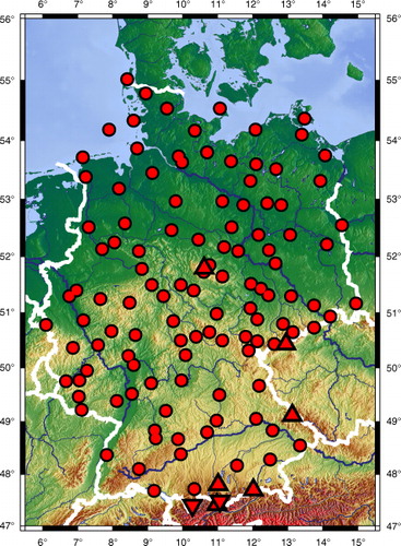
The locations of the measurement sites are shown in Fig. 1. The topographic environment of the stations varies from open sea and coastal sites to high mountain ranges. As topography and urban areas influence the mean wind speed, the roughness length z ₀ is determined through a gustiness analysis according to Wieringa (1986) and an exposure correction is performed for each measurement site (see also Verkaik, 2000). All measured wind speeds are corrected to a roughness length of 0.03 m as recommended by WMO (2008). The correction leads to a rescaling of the amplitude of mean wind speed and makes distributions of different sites comparable.

Fig. 1 Area of investigation and location of test sites. Triangles indicate mountain sites, diamonds indicate valley sites. Detailed information on test sites are presented in Supplementary file.

Once the initial roughness length is known by the gustiness analysis, the measured mean wind speed u _m can be extrapolated from the anemometer height z _m =10 m above ground to particular level z _b . At this level, called blending height, the wind speed is assumed to be horizontally constant. The blending height is set to 60 m (Wieringa, 1986; Verkaik, 2000).1

This wind speed u _b can be transformed back downwards to z _m but with a uniform roughness length z _0ref of 0.03 m, and is then called potential wind, u _p .2

The potential wind speed represents the rescaled uniform mean wind speed without local effects. As the exposure correction uses the logarithmic wind profile, the method can lead to biases in high mountain sites.

3. Wind gust model

3.1. Theory

In the following section, the theoretical concept of the wind gust model is explained. The model uses linear relationships between the statistical distributions of gust and rescaled wind speeds to derive gust distributions from known distributions of wind speeds.

Wind and gust velocities are modelled through a Weibull distribution. The cumulative probability function is described as follows:3

with F the cumulative Weibull distribution function of the variable u, a the scale parameter and b the shape parameter. In our case u can be wind or gust speed. The function can be linearized the following way:4a 4c

The result is a linear relationship between the two parameters of the Weibull distribution valid for every u. If wind speed can be modelled through a Weibull distribution, this relationship is valid for every theoretical distribution fitted to measured wind speed. This also implies that the linear coefficients m and n are the same for every distribution of wind speed. According to this thesis, one should be able to obtain m and n by combining Weibull parameters a, b of multiple distributions at several measurement sites and performing a linear regression. The Weibull distribution parameters can be obtained through a distribution fit on measurements at each site.

By applying the linear relationship on the distributions of gust speed and exposure corrected wind speed, we gain two independent linear equations [eqs. (5b) and (5c)]. A third equation is needed to connect the two equations and derive a distribution of gusts from wind speeds.

As gusts arise from fluctuations of wind, their Weibull distribution should have a similar shape parameter but a different scale parameter [eq. (5a)]. By combining this deduction with the linear relationship from eq. (4c) for wind and gust speed, it is possible to derive distribution parameters a _g and b _g of gust speed from distribution parameters a _w and b _w of wind speed by solving three equations.5a 5b 5c

Here, m and n mark the regression coefficients. The subscript marks the applied data basis, m _w , n _w for wind speed, m _g , n _g for gust speed and m _wg , n _wg in the equation combining the shape parameters of both measures. Equations (5b) and (5c) state that the Weibull distribution parameters of average wind speed and gust speed are linear to each other, while eq. (5a) states that the shape parameters of both measured variables are also linear. Knowing the distribution parameters of gust velocities, synthetic gusts can be derived for particular wind speeds through quantile–quantile mapping (Zhang et al., 2006; Haas and Born, 2011).6

Here u _w is the wind speed and u _g the gust speed. Considering a Weibull distribution for wind and gust speed, the equation reduces to7

The distribution parameters a _w and b _w can be gained from a Weibull fit on wind speed. The distribution parameters of gust speed a _g and b _g can be derived through eqs. (5a)–(5c) after calibration. One transfer function is determined separately for each location. Using the transfer function, for every mean wind speed observation, a corresponding gust estimation is determined. For this method, the availability of the entire spectrum of velocities is essential as the absence of lower gust speeds would result in different distribution parameters.

3.2. Calibration

The applicability of the model depends on the verification of the linear relationship between the two Weibull distribution parameters In a and b. This needs to be calibrated using measurement data. We distinguished four sectors of wind direction to take possible roughness length differences into account, while retaining a sufficient amount of data for a distribution fit. The results are shown exemplary for the west sector. Figure 2 shows scatter plots of the scale parameters In a _g , In a _w versus the shape parameters b _g , b _w for gust speed and exposure corrected mean wind speed, respectively. Other sectors are summarized in Table 1.

Fig. 2 Linear relationship of the distribution parameters In a and b for (a) wind speed and (b) gust speed based on hourly measurements. Mountain sites (green) and valley sites (cyan) are highlighted.

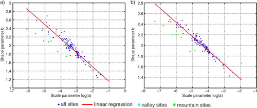
Both measures show sufficient agreement with the theoretical linear relationship. As the quality of the fit is dependent on the number of measurements, the anti-correlation is lowest for winds and gusts from the northerly sector and highest for the westerly sector (Table 1). The distribution parameters of westerly winds and gusts additionally show the lowest spread of all sectors (Supplementary file). The range of the shape parameter b is similar for westerly mean wind and wind gust speeds.

Table 1. Regression parameters of the relationship between distribution parameters In a and b for wind and gust speed dependent on the wind sector

North		East		South		West
Wind	Gust	Wind	Gust	Wind	Gust	Wind	Gust
Rel. freq.	17%		20%		27%		36%
Correlation	−0.79	−0.80	−0.88	−0.91	−0.75	−0.79	−0.90	−0.93
Slope	−0.30	−0.25	−0.34	−0.28	−0.28	−0.24	−0.33	−0.27
Offset	1.10	1.10	1.03	1.03	1.12	1.09	0.82	0.84

Mountain sites show larger deviations from the regression due to the bias from the insufficient exposure correction. Still, mountain sites form their own cluster of stations below the main regression. Valley stations show deviations depending on the orientation of the valley axes. If the valley orientation is aligned with a particular wind sector, the distribution parameters are in agreement with main regression. However, for other wind sectors the frequency of the wind measurements may be too low for a convincing distribution.

3.3. Cross-validation of synthetic gusts

The performance of the model has been tested with leave-one-out cross-validation. The gust distribution parameters estimated from wind speeds are compared to the maximum-likelihood estimated parameters of the measured gusts separately at each measurement site (for the west sector, Fig. 3). The results for the other sectors are summarized in Table 2. The scale parameter of the west sector shows an excellent correlation of 0.98 (Fig. 3a). All other wind direction sectors show almost no systematic errors, while shape parameters show a slight underestimation through the regression model (Supplementary file). Due to the higher occurrence frequency of the westerly wind sector, the correlation of 0.91 for this sector is the best for the shape parameters (Fig. 3b, Table 2). In terms of covariance, the west sector also performs best (Table 2). The underestimation of shape parameters can lead to an underestimation of high gust values.

Fig. 3 Validation of the original against estimated distribution parameters for (a) scale parameter and (b) shape parameter. The original distribution parameters are based on the maximum-likelihood estimation (MLE) of the original dataset of gust measurements. The estimations are derived by the wind gust model using measurements of wind speed. Mountain sites are highlighted in green, valley sites in cyan.

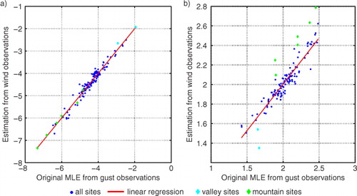
Table 2. Validation of distribution parameters In a and b of measurements versus estimations dependent on the wind sector

North	East	South	West
Scale	Correlation	0.97	0.98	0.98	0.98
Slope	1.001	1.001	0.999	0.999
Offset	0.004	0.002	0.000	−0.002
RMSE	0.20	0.18	0.18	0.16
Shape	Correlation	0.71	0.87	0.75	0.91
Slope	0.599	0.802	0.703	0.948
Offset	0.798	0.420	0.616	0.106
RMSE	0.16	0.14	0.16	0.10

There are deviations of the shape parameter for high mountain and valley sites due to the bias from the exposure correction concerning these stations in the model. The shape parameters of the mountain sites are underestimated while valley stations are overestimated.

The estimated parameters were used to generate gust time series by the use of quantile mapping [eq. (6)]. The root-mean-square error (hereafter RMSE) is used to quantify the accuracy of the estimated gusts in comparison to measurements. Results are shown in Fig. 4. Except for mountain and coastal stations, the RMSE of the estimated gusts range between 1 and 1.5 ms⁻¹. Coastal sites have a slightly higher RMSE (between 1.3 and 1.7 ms⁻¹) than inland sites, which is attributed to the high roughness variability of the sea. The spatial distribution of RMSE indicates that in most cases, the quantile mapping is able to compensate the underestimation of the shape parameter from the wind–gust relationship.

Fig. 4 RMSE of estimated gusts compared to measured gusts for the test sites.

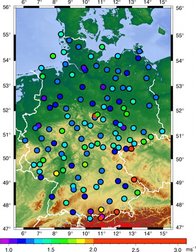
Due to the model bias, mountain sites show a higher RMSE than the rest of the sites. The largest RMSE is 3.06 ms⁻¹ at the Zugspitze, Germany's highest mountain, while the lowest RMSE is below 1 ms⁻¹ in Garmisch-Partenkirchen, a nearby valley site. The RMSE of the valley station is slightly below the precision of the data basis. The axes of the valley lead to a strong channelisation of the winds and a high predictability. In general, this example shows that with sufficient data basis of wind speed, direction and roughness length, the mean error can be reduced to a minimum.

4. Estimation of return periods

4.1. Extreme value statistics – theory

In terms of wind gust measurements, their extremes are of particular interest. Such extremes can be described with the help of extreme value statistics (Coles, 2001).

To prove the consistency of the estimated gusts and to introduce one possible application, an extreme value analysis following van den Brink and Können (2008, hereafter vdBK) is performed (see also van den Brink and Können, 2009). For this purpose, the statistical distribution of outliers and their return values of measured and estimated gusts are compared. VdBK introduced an approach based on the highest value of an observational record to examine its deviation from the underlying distribution. This deviation is a measure of the exceptionality of a particular gust, which can also be used to determine its return period. As this deviation is different for each measurement site depending on the local climatology, this approach provides an advantage to threshold-using methods (like POT, see Coles, 2001). In the context of gust return values, this means that a high gust at a coastal site (e.g. 40 ms⁻¹) can have a shorter return period than a comparatively lower gust (e.g. 35 ms⁻¹) in a valley. As only the highest value per record is used, the gust values have to be checked and classified as reliable.

VdBK considered 10 m wind speeds from the ERA40-reanalysis for their study. Here, we use real wind gust measurement data. While the use of measurements can lead to inaccuracies due to the shortness of the datasets and observation errors, it is the first time that this approach is applied to real data. As our objective is to evaluate the consistency of the estimated gusts with measurements, observation errors do not play a large role in our approach. VdBK verified the hypothesis of Cook (1982) that the standardized annual maxima of wind speed follow a Gumbel distribution if is the fitted variable, with a the scale and b the shape parameter of the Weibull distribution. The return period T of an extreme event is usually formulated through its probability.8

Here, F is the cumulative distribution of the annual maxima of the variable y at one test site. The distribution can be seen as a local climatology of annual maxima. According to Cook (1982), F should be the Gumbel distribution for maxima of a Weibull distribution,9

where µ is the location parameter and α the scale parameter of the Gumbel distribution. Consider y _n is the maximum of an observational record of n independent annual maxima then the distribution of y _n can be expressed as follows:10

F(y _n ) is the cumulative probability function and T _n the return period of y _n . By applying the negative logarithm on both sides of the equation twice, we obtain:11

The right side of the equation can be defined as ΔX _n . This variable can be interpreted as the deviation of certain maxima from the underlying climatology. Thus, a high ΔX _n means that the particular gust is rare for local conditions, corresponding to a high return period. Conversely, a low ΔX _n indicates a low return period. The reason can be a low magnitude of the particular gust, or the underlying distribution indicating a high frequency of high gust speeds. The magnitude of ΔX _n depends on the distribution F and on the rank of the particular maximum n. By applying the exponential function twice on both sides of the equation, we get the following expression:12

For independent annual maxima, ΔX _n follows the standardized Gumbel distribution with location parameter µ=0 and scale parameter α=1. In terms of gust speed, spatial and temporal independence implies that the gusts occur during different events. The scaling of the variable by the rank of maxima allows combinations of different observation records at different locations. The measurement periods do not need to cover the same time span nor do they need to be of the same length. The combination of different observation records allows additional spatial investigations.

In practice, the following steps are carried out: Firstly, we determine the annual gust maxima at every measurement site. The annual maxima are scaled by the local parameters of the Weibull distribution. To receive ΔX _n from eq. (11), a Gumbel distribution [i.e. F(y)] is fitted to the annual maximum gusts at each site. The ranks of the gusts (n, i.e. number of years) are also required. Secondly, the resulting maximum ΔX _n of different sites are compared. If one event sets the maximum ΔX _n for multiple sites, only the highest ΔX _n is considered. The distribution of the resulting independent maximum ΔX _n should then follow a standardized Gumbel distribution. The obtained return period is specific for the particular measurement site and the local climatology at this point. As only the maximum ΔX _n per event is taken into account, the obtained return period is valid for only one test site, which has been affected by the given event. We refer to it as the maximum return period.

In the case of large-scale events like intense extratropical cyclones (windstorms), the interest is focused on the large areas affected by wind gusts and the event-specific return periods. In this case, average return periods are required. For this purpose, we extend the approach of vdBK through collecting ΔX _n of all stations affected by a selected windstorm to obtain an extreme value distribution. In contrast to the previous application, we change the reference period keeping the event fixed, meaning that lower return periods are also considered. In practice, the maximum gust during a selected time interval around the windstorm passage must be determined. This gust is compared to the location-specific climatology in order to receive ΔX _n and thus its return period. For an exemplary windstorm Kyrill, which crossed Germany on 18 Jan 2007 (Fink et al., 2009), we choose ΔX _n of all stations associated with this date. As all stations were affected, thus the distribution of ΔX _n consists of 123 values. As ΔX _n values of one particular event are neither temporally nor spatially independent, the Gumbel distribution of ΔX _n receives an event-specific location parameter µ _e and scale parameter α _e and is applied on every station affected by the selected storm.13

The median value of the distribution of ΔX _e describes the average return period T _e of an event.

In our context, the performance of estimated gusts during extreme events is of interest. In particular, the distribution of annual maxima of estimated gusts should be comparable with the distribution of annual maxima of measurements. The most extreme events based on measurements are expected to be included in both distributions.

4.2. Determination of the distribution

In order to verify the adequacy of the standardized Gumbel distribution for extreme gusts, we determined ΔX _n for each data record. If a large-scale event caused a maximum for several sites, only the highest ΔX _n was considered for the distribution, in order to ensure temporal and spatial independence. To distinguish between different events, two gusts need to be separated by a minimum interval of 24 hours. Due to the comparatively small area of investigation, no spatial threshold for multiple footprints is required (cf. Haas and Pinto, 2012; Pinto et al., 2012). The return periods derived from this method consider only the highest gust in terms of local conditions.

The procedure was conducted on the measured and estimated gust dataset separately in order to compare the results. Figure 5a shows Gumbel plots of ΔX _n for measured gust velocities. The parameters of the Gumbel distribution of this dataset (µ= −0.39, α=1.02) agree highly with theoretical expectations mentioned in eq. (12). The distribution of ΔX _n converges to the Gumbel distribution in agreement to vdBK. Still, there is an additional location parameter due to the short length of observational records (cf. deviation in Fig. 5a). The three highest events agree less well with the rest of the distribution. Possible reasons are, aside from the record length, associated with the physical nature or location of the events. We will analyse this aspect in Section 5.2.

Fig. 5 Gumbel-plot for (a) measurements and (b) estimates and maximum return periods of locally strongest gusts identified in the dataset of (c) measurements and (d) estimations. The blue dots in the Gumbel plots (a, b) indicate ΔX _n for independent extreme events based on all wind sectors, the red line shows the theoretical distribution, while the cyan lines show the 95% of the confidence intervals of ΔX _n estimation. The blue dots in (c) and (d) indicate the return periods and their 95% confidence intervals for all wind sectors, while for red dots only the west sector was taken into account.

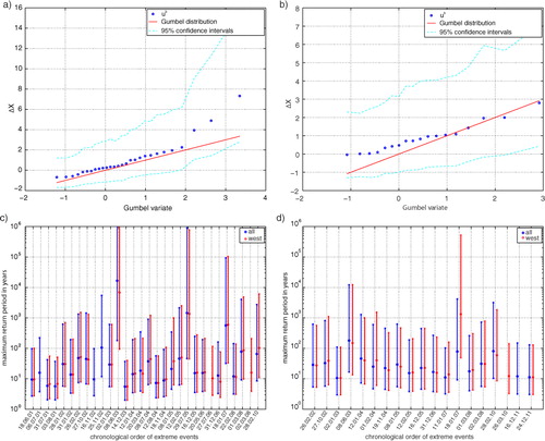
The parameters of the Gumbel distribution based on estimated gusts (µ=−0.54, α=0.57) agree less well with the theoretical distribution than the measured dataset (Fig. 5b). Both parameters deviate from the standardized distribution. Figure 5b shows that there are fewer events determined than for measured datasets. It is also noticeable that the range of ΔX _n is lower compared to measurements with larger deviations for low ΔX _n and smaller deviations for higher ones. The main reason for this discrepancy is the high sensitivity of the fit of the Gumbel distribution to local annual gust maxima, as the record length is only 11 yr. Thus, low uncertainties of individual estimations can result in uncertain distribution parameters. Possible consequences are under- or overestimation of local climatologies and thus of ΔX _n . This leads to a different choice of the maximum ΔX _n and maximum return values.

4.3. Maximum return periods of gust maxima

The methodology applied to the measurements leads to the identification of 28 independent extreme events (Supplementary file). About two-thirds (20 events) of the events occurred during the winter season and one-third (eight events) during summer. The three strongest events, which clearly deviate from the distribution leading to extraordinary high return periods, are two summer events (8 June 2003; 29 July 2005) and the storm Kyrill (18 January 2007, see Fink et al., 2009). All winter events are extratropical cyclones, while summer events are intense thunderstorms. The maximum return periods for all of the 28 events are also shown in Fig. 5c. Almost all extreme events are associated with winds from the westerly wind sector. There are only marginal differences in terms of return periods between the analyses of all wind directions compared to west winds. The eight summer events have been identified as European Derechos (six events) or Bow Echos (C. Gatzen, personal communication, 24 June 2013). Additionally, the two strongest winter events, Kyrill (18 January 2007) and Emma (1 March 2008), were accompanied by Derechos (Gatzen et al., 2011).

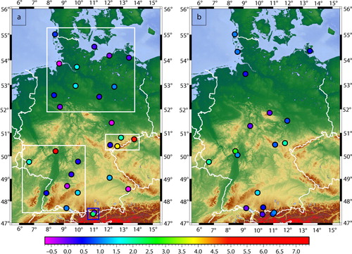
The locations of the sites where the 28 analysed extreme gusts were identified are shown in Fig. 6a. There are three main regions with aggregation of extreme gusts (white boxes). The most extensive region is in the north of Germany, which is frequently affected by extratropical cyclones. Ten out of 11 extreme events appeared during the winter season. The range of ΔX _n is medium to low compared to the overall range. The second region is in the southwest of Germany. Here, the origin of extreme gusts is balanced between summer and winter events. With the exception of one site, the range of ΔX _n is similar to northern Germany. The most extreme events have been measured in mountainous regions, which is also verified in the third aggregation region near the Erzgebirge in eastern Germany. The three highest events, which clearly deviate from the overall distribution, appeared in such mountainous regions. These gusts were possibly generated through extraordinary strong down-mixing of momentum during the passage of the extreme events (cf. Fink et al., 2009, on Kyrill). The only three events, when gusts came from the south sector, occurred in the south of Germany. Two of them were Foehn storms (Fig. 6a, blue box) in the alpine region. The location of the third station is in the upper Rhine valley, whose axis has a north-south orientation, which limits the influence of westerly winds.

Fig. 6 Locations of occurrences of extreme gusts (maximum ΔX _n ) for all directions for (a) measurements and (b) estimations from wind speeds. The white boxes mark the three main aggregations of extreme events shown in Fig. 5c. The blue box indicates the position of the two Foehn gusts.

For estimated gusts, only 18 independent events have been identified (Supplementary file). In this case, events occurred mostly in combination with large-scale extratropical cyclones, as only the highest summer Derecho event (8 June 2003) is included. As the wind speed is the only predictor for the gust estimation in the wind gust model, high gusts are always accompanied by high wind speeds. This seems to work fine in the case of large-scale cyclones, but less well in the case of convective summer events. Thus, there are only small differences in terms of return periods between all wind directions vs. west winds both for measured and estimated gusts except for the summer event (Fig. 5c–d), as windstorms typically cause westerly winds.

The comparison of Fig. 5c–d shows that 11 events can be identified with both measured and estimated gusts. Still, the differences in return periods between measurements and estimations range between 2 yr for Jeanett (27 October 2002) and several decades (cf. Supplementary file). There are additional differences between extreme events based on measured and estimated gust records. In four cases, the occurrence of multiple storms per year leads to deviations in the return periods, since the local annual maximum may have been associated with another storm. This is, for example, the case for the winter season 2003–2004.

The spatial distribution of ΔX _n does not represent the three above-mentioned aggregation regions correctly (Fig. 6). Here, the reason is a high sensitivity of Gumbel distribution parameters for the different measurement sites. The estimation of the maximum return period is based on the maximum ΔX _n per station and distinct event. As the bias is different for every site, the maximum ΔX _n can be reached at a different site to that of the original measurement records, which results in a different maximum gust, local climatology and return value.

4.4. Average return periods of large-scale events

In order to reduce discrepancies mentioned in the previous subsections and to provide relevant information for impact studies, average return periods are determined. We use the same concept as in Section 4.3, but instead of independent maxima we study the distribution of ΔX _n during particular events, which were identified in Section 4.3 and listed in Supplementary file. In order to avoid focusing on very local events (thunderstorms), only events affecting a ‘considerable’ area were taken into account. This means that at least 10 stations need to be affected by a given event. Convective events were thus excluded due to the limited affected area, the associated underrepresentation in estimations and the high temporal and spatial gust variability.

To derive average return periods for a given event, all gust maxima per station and event are required. Based on the maximum gusts from Section 4.3, we choose a 36-hour period covering 18 hours before and after the maximum gust of the selected event occurred. For every measurement site, the maximum gust occurred during this time period is selected and the ΔX _n of the selected gust is determined. As ΔX _n depends on the rank of the gust, the maximum gust would be lower than all annual maxima in the climatology (i.e. if a measurement site was not affected by the particular storm, its rank will be zero). By applying this restriction no distance thresholds are necessary. For all other cases, ΔX _n of the site is included in the storm-specific distribution. The distribution parameters of ΔX _n for each storm event were estimated by using the maximum-likelihood method. The distribution of ΔX _n is used to calculate the median value of ΔX _n and its return period.

The average return periods are presented in Fig. 7 and Table 3. With the exception of the three strongest events (Kyrill, Jeanett and Emma), all average return periods cover the range between 2 and 7 yr, which is several decades lower than the maximum return periods. The results for the three strongest events are consistent with the range of return periods estimated by Donat et al. (2011) based on loss data. For certain events (Kyrill, Jeanett, Emma and Erwin), the return periods based on measurements show higher differences between the overall distributions and the west sector than return periods based on estimations. A possible reason might be a smoothing of the gust distributions due to the wind–gust model, which also includes the extremes and their climatology.

Fig. 7 Average return periods of extreme events in chronological order for (a) measurements and (b) estimations from wind speeds. Blue dots indicate the data basis of all directions, while red dots are based on the west sector only. Detailed estimates are presented in Table 3.

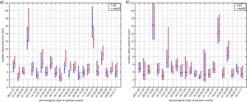
Table 3. Median return periods (Med. rp) of large-scale extreme events based on measurements and estimated gust values for all wind sectors. Events identified only from estimated gusts are marked with asterisks.

Event names	Date	Med. rp meas. (years)	Range meas. (years)	Med. rp est. (years)	Range est. (years)
Anna	26.02.2002	4.17	3.59–5.19	4.37	3.55–5.81
Jennifer	28.01.2002	5.07	4.06–6.88	4.83	3.90–6.47
Lydia	31.01.2002	2.47	1.79–3.62	3.24	2.12–7.55
Jeanett	27.10.2002	12.05	9.93–15.74	16.28	12.58–22.50
Calvann	02.01.2003	4.34	3.18–6.23	4.31	3.14–6.14
Fritz	14.12.2003	3.19	2.47–5.02	2.96	2.11–4.74
Gerda	12.01.2004	5.23	3.90–8.98	6.41	5.20–9.72
Queenie*	01.02.2004	3.84	2.99–5.27	5.05	3.95–6.74
Oralie	20.03.2004	5.68	4.71–8.06	5.60	4.53–7.06
Pia	18.11.2004	3.50	2.74–5.03	3.73	2.87–5.62
Quimburga*	19.11.2004	2.63	1.72–4.99	3.95	2.31–7.94
Erwin	08.01.2005	4.74	3.82–6.54	3.99	3.33–5.38
Ulf	12.02.2005	3.22	2.64–4.50	3.29	2.72–4.25
Dorian	16.12.2005	4.79	3.85–6.03	2.53	2.22–3.28
Gertrud	20.05.2006	3.03	1.97–5.52	3.35	1.72–9.82
Karla	31.12.2006	3.90	2.65–5.49	3.42	2.62–4.57
Franz*	11.01.2007	4.33	3.34–6.02	4.88	3.85–6.71
Kyrill	18.01.2007	16.09	12.97–20.98	14.06	11.56–18.12
Annette	22.02.2008	4.16	3.13–6.79	3.20	2.49–4.79
Emma	01.03.2008	7.28	6.04–9.30	8.28	6.88–10.56
Fee	02.03.2008	3.83	2.85–5.00	3.12	2.53–4.60
Xynthia	28.02.2010	4.13	3.59–5.14	4.87	3.99–6.07
Joachim*	16.12.2011	3.47	2.61–5.72	3.40	2.64–5.09

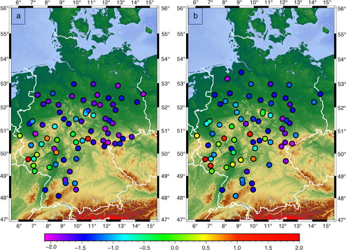
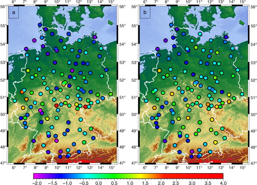
Figure 8 shows spatial distributions of ΔX _n during the passage of the event ‘Xynthia’ at 28 February 2010 (Liberato et al., 2013). For comparison, the complete windstorm footprint obtained with the COSMO-CLM regional climate model is shown in Haas and Pinto (2012), their Figure 1d. The spatial distribution based on measured gusts shows a south-west to north-east orientation in terms of magnitude of ΔX _n . Neither coastal regions nor the Alps were severely affected by the storm. The most exceptional gusts occurred in the southwest close to the French border and in exposed areas in low mountain ranges. The gust (35 ms⁻¹, cf. Supplementary file) with the maximum return period occurred at the measurement site of Trier-Petrisberg. The spatial distribution of estimated extremes shows a similar south-west to north-east orientation as measurements (Fig. 8). Most of the extreme gusts are also focused in the south-west. The location of the gust with the maximum return period agrees well with measurements. The associated gust speed is 37 ms⁻¹ (cf. Supplementary file), which is only slightly above the measured gust speed. The spread of the overall distribution is larger for estimated gusts and there are some stations in the north and southeast, which were additionally captured by the estimated storm. There is a tendency towards overestimation of modelled gusts for the northern and southern part of the spatial distribution.

Fig. 8 Spatial distribution of ΔX _n during the storm Xynthia (28 Feb 2010) for (a) measured and (b) estimated gusts.

The storm Kyrill (18 January 2007) shows a different spatial distribution (Fig. 9) compared to Xynthia. The storm affected the whole investigation area, which is confirmed by measurements as well as estimations (see also full footprint in Haas and Pinto (2012), their figure 1c). The measured gusts with the highest return periods are focused in the middle part of Germany with highest values in the mid-range mountains and the west of Germany. The gust of 36 ms⁻¹ with the highest return period occurred at the Carlsfeld site in the east of Germany. The gusts with lowest return periods occurred near the coasts and in the south-west. The range of ΔX _n varies from −2.03 to 3.94 (corresponding to 28–36 ms⁻¹). However, it should be noted that the largest observed gust 56 ms⁻¹ was not considered as it was low compared to the local maxima. For estimations, the gusts with highest return periods also occurred in middle Germany and in the south-east. The gust with the highest return period of 38 ms⁻¹ occurred also in the east of Germany, but at a different site. The parts with the lowest return periods are, as for measurements, in the south-west and in coastal regions. Still, the range of estimated ΔX _n is smaller, ranging from −1.75 to 1.97 (corresponding to 20–38 ms⁻¹). In this example, the distributional smoothing is obvious through locally lower and less peak gusts, but higher mid-range gusts. The impression of distribution smoothing, gained in former results, has been confirmed in both examples.

Fig. 9 Spatial distribution of ΔX _n during the storm Kyrill (18 Jan 2007) for (a) measured and (b) estimated gusts.

5. Conclusions

We developed a new wind gust model to derive synthetic wind gusts from mean wind observations. This was achieved by establishing a relationship between the distribution parameters of mean wind and gust speeds. Exposure correction was performed using the roughness length of the surrounding area of the measurement site to obtain comparable statistics for all stations. The corrected wind speeds and gust observations are then used to build the wind gust model. The gust estimation may contain error sources like deviations of distribution parameters from the linear relationship or a distortion of the distributions through the probability mapping. Nonetheless, the mean RMSE of 1.36 ms⁻¹ of estimated gusts is only slightly above the precision of the gust measurements. Only sites with complex surrounding topography or varying roughness show higher deviations.

In an exemplary application of the wind gust model, which could also be considered as an additional validation, measured and estimated gusts are used to calculate return periods. Estimates are achieved for both the maximum return period (location specific) and the average return period (event specific). The distribution of measured extreme gusts is in agreement with the theory described in van den Brink and Können (2008, 2009). There are only three events which deviate from the theoretical distribution, resulting in a more uncertain estimation of return periods. All three maximum gusts occurred in mid-range mountain areas with complex topography and during two summer Derecho events or storm Kyrill with an embedded Derecho. The comparison of maximum and average return periods shows that although only three winter storms (Kyrill, Jeanett, Emma, with return periods between 7 and 16 yr) caused extraordinary strong gusts throughout whole Germany, weaker storms with lower average return periods may lead to local wind gusts with return periods of several decades. The investigation of average return periods showed that the range of extreme gusts is consistent with measurements and with estimates by Donat et al. (2011) based on historical loss data.

The gust estimation based on wind measurements leads generally to realistic and consistent values. This is particularly the case for large-scale events like winter storms which affect large parts of Germany. The method performs less well for localized events. The distributional smoothing hardly affects average return periods of large events, while the estimates for smaller and weaker events might be overestimated. The smoothing can also affect the magnitude of estimated gusts, producing a right skewed gust distribution with a smaller range. This can cause erroneous values of annual gust maxima as well as their distribution parameters, leading to erroneous estimates of maximum return periods.

In terms of possible enhancements of the methodology, longer records would allow a subdivision of more wind sectors and to get more detailed roughness information, which could additionally reduce the RMSE in our wind gust model. Additional data records in upper mountain ranges would also improve estimations for mountain sites. Although the van den Brink and Können (2008, 2009) approach is able to estimate return periods beyond the length of the time series, it requires a large amount of consistent data records as only one value per record and event is used. Future investigations should thus include an enlarged dataset to overcome the caveats associated with the length of the time series. Additional parameters could be helpful to improve the estimation of gusts for thunderstorms.

The results of the present study enable a wide range of possible applications. For example, this methodology may help to better estimate the windstorm risk and wind energy potentials over Europe under recent and future climate conditions, also in areas with less available wind gust observations. In the same line of thought, the return periods of historical storms can now be estimated directly from observational data in a multinational perspective and independently from loss estimation.

6. Acknowledgements

We thank Frank Kaspar and the German Weather Service (DWD) for providing the wind and gust speed data. This research was supported by the German Federal Ministry of Education and Research (BMBF) under the project Probabilistic Decadal Forecast for Central and Western Europe (MIKLIP-PRODEF, contract 01LP1120A). We thank C. Gatzen (Meteogroup) for information related with Derechos in Germany and M. Reyers (University of Cologne) for discussions. We also thank two anonymous reviewers for their helpful and constructive comments.

Notes

To access the supplementary material to this article, please see Supplementary files under Article Tools online.

References

- An Y , Panley M. D . A comparison of methods for extreme wind speed estimation. J. Wind Eng. Ind. Aerod. 2005; 93: 535–545.
- Barthelmie R. J , Murray F , Pryor S. C . The economic benefit of short-term forecasting for wind energy in the UK electricity market. Energy Policy. 2008; 36: 1687–1696.
- Beljaar A. C. M . The influence of sampling and filtering on measured wind gusts. J. Atmos. Ocean. Technol. 1987; 4: 613–626.
- Born K , Ludwig P , Pinto J. G . Wind gust estimation for Mid-European winter storms: towards a probabilistic view. Tellus A. 2012; 64: 17471.
- Brabson B. B , Palutikof J. P . Test of the generalized Pareto distribution for predicting extreme wind speeds. J. Appl. Meteorol. 2000; 39: 1627–1640.
- Brasseur O . Development and application of a physical approach to estimating wind gusts. Mon. Weather Rev. 2001; 129: 5–25.
- Brayshaw D. J , Troccoli A , Fordham R , Methven J . The impact of large scale atmospheric circulation patterns on wind power generation and its potential predictability: a case study over the UK. Renew. Energy. 2011; 36: 2087–2096.
- Coles S . An Introduction to Statistical Modeling of Extreme Values. 2001; Coles, S. Springer, London..
- Cook N. J . Towards better estimations of extreme winds. J. Wind Eng. Ind. Aerod. 1982; 9: 295–323.
- Della-Marta P. M , Liniger M. A , Appenzeller C , Bresch, D. N. Köllner-Heck P , co-authors . Improved estimates of the European winter wind storm climate and the risk of reinsurance loss using climate model data. J. Appl. Meteorol. Clim. 2010; 49: 2092–2120.
- Della-Marta P. M , Mathis H , Frei C , Liniger M. A , Kleinn J , co-authors . The return period of windstorms over Europe. Int. J. Climatol. 2009; 29: 437–459.
- Donat M. G , Pardowitz T , Leckebusch G. C , Ulbrich U , Burghoff O . High-resolution refinement of a storm loss model and estimation of return periods of loss-intensive storms over Germany. Nat. Hazards Earth Syst. Sci. 2011; 11: 2821–2833.
- Fink A. H , Brücher T , Ermert V , Krüger A , Pinto J. G . The European Storm Kyrill in January 2007: synoptic evolution and considerations with respect to climate change. Nat. Hazards Earth Syst. Sci. 2009; 9: 405–423.
- Friedrichs P , Göber M , Bentzien S , Lenz A , Krampitz R . A probabilistic analysis of wind gusts using extreme value statistics. Meteorol. Z. 2009; 18: 615–629.
- Gatzen C , Púčik T , Ryva D . Two cold-season derechoes in Europe. Atmos. Res. 2011; 100: 740–748.
- Gerth W , Christoffer J . Wind charts of Germany. Meteorol. Z. 1994; 3: 67–77.
- Haas R , Born K . Probabilistic downscaling of precipitation data in a subtropical mountain area: a two-step approach. Nonlinear Process. Geophys. 2011; 18: 223–234.
- Haas R , Pinto J. G . A combined statistical and dynamical approach for downscaling large-scale footprints of European windstorms. Geophys. Res. Lett. 2012; 39: L23804.
- Harris I . Generalized Pareto methods for wind extremes. Useful tool or mathematical mirage?. J. Wind Eng. Ind. Aerod. 2005; 93: 341–360.
- Hueging H , Born K , Haas R , Jacob D , Pinto J. G . Regional changes in wind energy potential over Europe using regional climate model ensemble projections. J. Appl. Meteorol. Climatol. 2013; 52: 903–917.
- Kasperski M . A new wind zone map of Germany. J. Wind Eng. Ind. Aerod. 2002; 90: 1271–1287.
- Liberato M. L. R , Pinto J. G , Trigo R. M , Ludwig P , Ordóñez P , co-authors . Explosive development of winter storm Xynthia over the southeastern north Atlantic ocean. Nat. Hazards Earth Syst. Sci. 2013; 13: 2239–2251.
- Pinto J. G , Karremann M. K , Born K , Della-Marta P. M , Klawa M . Loss potentials associated with European windstorms under future climate conditions. Clim. Res. 2012; 54: 1–20.
- Pryor S. C , Barthelmie R. J . Climate change impacts on wind energy: a review. Renew. Sustain. Energ. Rev. 2010; 14: 430–437.
- Schwierz C , Köllner-Heck P , Mutter E. Z , Bresch D. N , Vidale P.-L , co-authors . Modelling European winter wind storm losses in current and future climate. Clim. Change. 2010; 101: 485–514.
- Van de Vyver H , Delcloo A. W . Stable estimations for extreme wind speeds. An application to Belgium. Theor. Appl. Climatol. 2011; 105: 417–429.
- van den Brink H. W , Können G. P . The statistical distribution of meteorological outliers. Geophys. Res. Lett. 2008; 35: L23702.
- van den Brink H. W , Können G. P . Estimating 10000-year return values from short time series. Int. J. Climatol. 2009; 31: 115–126.
- Verkaik J. W . Evaluation of two gustiness models for exposure correction calculations. J. Appl. Meteorol. 2000; 39: 1613–1626.
- Walter A , Keuler K , Jacob D , Knoche R , Block A , co-authors . A high resolution reference data set of German wind velocity 1951–2001 and comparison with regional climate model results. Meteorol. Z. 2006; 15: 586–596.
- Wever N . Quantifying trends in surface roughness and the effect on surface wind speed observations. J. Geophys. Res. 2012; 117: D11104.
- Wieringa J . Roughness-dependent geographical interpolation of surface wind speed averages. Q. J. Roy. Meteorol. Soc. 1986; 112: 867–889.
- Wieringa J . Representative roughness parameters for homogeneous terrain. Boundary Layer Meteorol. 1993; 63: 323–363.
- WMO. 2008; Switzerland: Geneva. Guide to Meteorological Instruments and Methods of Observation. 7th ed Online at: http://www.wmo.int/ .
- Zhang L. F , Xie M , Tang L. C . A study of two estimation approaches for parameters of Weibull distribution based on WPP. Reliab. Eng. Syst. Saf. 2006; 92: 360–368.