Which significance test performs the best in climate simulations?

Abstract

Climate change simulated with climate models needs a significance testing to establish the robustness of simulated climate change relative to model internal variability. Student's t-test has been the most popular significance testing technique despite more sophisticated techniques developed to address autocorrelation. We apply Student's t-test and four advanced techniques in establishing the significance of the average over 20 continuous-year simulations, and validate the performance of each technique using much longer (375–1000 yr) model simulations. We find that all the techniques tend to perform better in precipitation than in surface air temperature. A sizable performance gain using some of the advanced techniques is realised in the model Ts output portion with strong positive lag-1 yr autocorrelation (> + 0.6), but this gain disappears in precipitation. Furthermore, strong positive lag-1 yr autocorrelation is found to be very uncommon in climate model outputs. Thus, there is no reason to replace Student's t-test by the advanced techniques in most cases.

• autocorrelation
• temporal correlation
• internal variability
• climate noise
• significance test
• Student's t-test

1. Introduction

Climate models are employed to simulate mean climatology as well as climate change. When the climate models simulate externally forced climate change (e.g. climate change induced by anthropogenic or natural radiative forcing), not only are the models simulating climate change due to this forcing but they also simulate internal variability due to the non-linearities in the climate system. Climate models always generate internal variability, and different initial conditions, different boundary conditions and radiative forcing influence this variability. Externally driven climate change is of principal interest in most cases but is often obscured by model internal variability. There is no method available yet to cleanly separate the externally driven climate change from internal variability, making interpretation of modelling results very challenging. From a statistical perspective, externally driven climate change can be considered signal and internal variability can be considered noise. Some examples of internal variability in an ocean-atmosphere coupled model are ENSO (El Niño-Southern Oscillation), PNA (Pacific–North American) variability and NAO (North Atlantic Oscillation).

Modellers attempt to reduce the impact of internal variability by generating more model output. A common approach to generating more output is to integrate a model over a long time period (say, 20 model years). The average over 20 yr of continuous model integration will contain relatively less variability. Another way of generating more output is to use a set of independent model runs (so-called ensemble simulations) that can be averaged as a whole. In both cases, Student's t-test is the most widely used technique to quantify the significance of the model output average relative to the variability of the average. The modeller needs multiple averages from multiple sets of, e.g. 20 yr of continuous simulation, in order to correctly estimate the significance of the average over a single 20-yr run, but is forced to guess the significance by using the same single 20-yr run alone. Statistical techniques such as Student's t-test use the temporal variation within the single 20-yr run to infer the significance. Relying on a single 20-yr run is the reason why these statistical techniques are subject to uncertainty. Here, we bypass the uncertainty in the significance estimated by these techniques, by obtaining multiple averages from nearly 1000-yr long runs, and thus validate the performance of the techniques.

In the present study, we investigate how correctly Student's t-test and other techniques estimate the significance of the average over 20 (or longer) years of continuous model integration. Making an average over 20~70 yr of climate model integration is a very common practice in case climate forcing is fixed over time (e.g. Chung et al., 2002; Jin et al., 2013). In this case, the modeller conducts a control run with basis forcing and carries out an experiment run with perturbed forcing. The contrast between the average over 20 yr of the control run and that over 20 yr of the experiment run yields the impact of forcing perturbation on climate. The contrast is typically shown for a particular season or calendar month, for instance as an average over December, January and February (DJF). When modellers estimate the significance of the DJF average over 20 yr by applying Student's t-test, the technique assumes an independence of 20 DJF averages (e.g. Kunkel et al., 2010; Wei et al., 2010).

To see if DJF averages are independent of each other in continuous climate simulation, we show autocorrelation between 1 yr DJF average and the next in Figs. 1 and 2. Autocorrelation is also referred to as serial or temporal correlation. As Fig. 1 shows, autocorrelation in Ts simulation ranges widely from −0.7 to +0.8. Autocorrelation in precipitation simulation ranges somewhat less widely (Fig. 2).

Fig. 1 Lag-1 yr autocorrelation in surface air temperature (Ts) averaged over December, January and February (DJF). Cross-hatched areas denote strong positive autocorrelation (>0.6). Autocorrelation is calculated on the long simulations in Table 2. Lag-1 yr autocorrelation represents the relationship between 1 yr and the next.

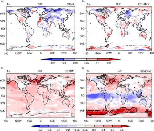
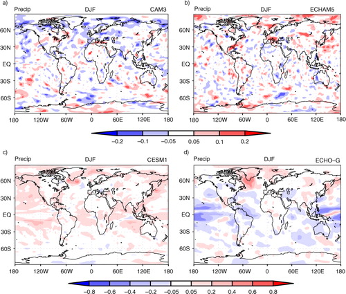
Fig. 2 Lag-1 yr autocorrelation in precipitation (precip) averaged over December, January and February (DJF). Autocorrelation is calculated on the long simulations in Table 2. Lag-1 yr autocorrelation represents the relationship between 1 yr and the next.

Since Student's t-test assumes independence of 20 DJF averages, the technique produces errors when there is lag-1 yr autocorrelation (Zwiers and Von Storch, 1995; Wilks 1997, 2011). A series of techniques have been developed to address autocorrelation with the aim to improve upon Student's t-test. Only a few methods have gained attention from the climate model community: the effective sample size t-test (Zwiers and Von Storch, 1995; Wilks, 1997, 2011), the moving blocks bootstrap test (Künsch, 1989; Wilks, 1997) and the pre-whitening bootstrap test (Solow, 1985; Efron and Tibshirani, 1993). Another assumption in Student's t-test is that 20-yr averages would be normally distributed. The so-called bootstrap test (Efron, 1982; Efron and Tibshirani, 1993) was developed to circumvent this assumption. However, it is not clear if these advanced techniques indeed improve upon Student's t-test in climate simulations. Some of these advanced techniques (i.e. the effective sample size t-test in Zwiers and Von Storch, 1995 and the moving blocks bootstrap test in Wilks, 1997) were tested or optimised using positively autocorrelated time series generated from time series models such as the autoregressive model (AR) or the autoregressive moving average model (ARMA). These time series models, by varying the coefficients, can exhibit various features. Realising this power, Zwiers and Von Storch (1995), for example, assumed that these models could approximate observed climate behaviours. In reality, only after choosing a suitable time series model and a set of particular coefficients, the time series model can at best replicate some aspects of the chosen climate model output, but not all the aspects simultaneously. This shortcoming of time series models is apparent in studies by Lee et al. (2011), Soltani et al. (2007) and Zwiers and Von Storch (1990), among many others. More importantly, the techniques were tested or optimised using positively autocorrelated time series, e.g. in Wilks (1997) and in Zwiers and Von Storch (1995), when autocorrelation is often negative in climate simulations, as evident in Figs. 1 and 2. Thus, it is very important to test these techniques using actual climate model simulations, and this is the goal of the present study.

Another aspect to consider is spatial correlation. When modellers apply Student's t-test to climate simulation, they do so either on each grid or on an area average. Applying the technique on each grid assumes that grids are independent of each other. This assumption is not correct, and attempts have been made to address spatial correlation (Zwiers, 1987; Elmore et al., 2006; Wilks, 2011). In this study, we only test the techniques as applied over an area average, in order to focus on temporal correlation. Area averages are more independent of each other than grid points.

Table 1 summarises to what extent Student's t-test and the four new techniques mentioned above have been used for significance tests in continuous climate model integrations in J. Climate publications from 2008 till 2011. In this survey, we only included the literatures where time series of a single grid point or area averages are considered. As displayed in Table 1, Student's t-test is by far the most popular technique. However, it is even more common to simply refrain from performing any significance test at all. This is partly because signal significance is often irrelevant to the research goals, e.g. when the focus lies on understanding how a model works. Even so, some studies which could benefit from significance tests were conducted without significance analysis (Mearns, 1997). The infrequent use of sophisticated techniques (other than Student's t-test) may be attributable to inaccessibility. The papers introducing new techniques tend to heavily use very abstract statistical terms such as ‘parametric test’, ‘asymptotic test’ ‘log-likelihood’ (more examples seen in studies by Zwiers, 1987; Wilks, 1997; Von Storch and Zwiers, 1999 and Zwiers and Thiébaux, 1987). These terms are difficult or unclear to most climate modellers. In the present paper, we attempt to avoid such terms to serve the climate model community. Another aspect of the inaccessibility is that relative to Student's t-test the other sophisticated techniques are difficult to implement. We summarise the implementation steps for these techniques in the Appendix.

Table 1. Survey of 3 yr of J. Climate publications (from 2008 to 2011) where significance tests are applicable on the average over a continuous climate model simulation^a

Technique	Number of relevant papers
No test	108 (49%)
Student's t-test	97 (44%)
Effective sample size t-test (modified Student's t-test)	13 (6%)
Bootstrap test	3 (1%)
Moving blocks bootstrap test and pre-whitening bootstrap test (modified bootstrap tests)	0 (0%)

^aThis table does not contain significance tests applied on ensemble runs.

Section 2 details the climate model runs used for analysis and summarises the methodology used to quantify the performance of the statistical techniques. Section 3 presents the results of the performance analysis. We discuss the performance results in Section 4. Conclusion follows in Section 5.

2. Model output and methodology

We analyse the output from CAM3 (Community Atmosphere Model Version 3.1; Collins et al., 2006), ECHAM5 (European Centre Hamburg Model Version 5.3; Roeckner et al., 2003), ECHO-G (ECHAM4 + Hamburg Ocean Primitive Equation – Global version; Zorita et al., 2003) and CESM1 (Community Earth System Model Version 1.0; Gent et al., 2011). As Table 2 explains, these models are ocean-atmosphere fully coupled models as well as atmospheric models forced by prescribed sea surface temperature seasonal cycle. All of the runs we analyse are subject to temporally fixed default forcing, so that there is no real trend in the runs. In case of fully coupled models ECHO-G and CESM1, the forcing was kept at pre-industrial conditions. To prevent spin-up effects from affecting the analysis, we remove the initial period. Table 2 shows the length of integrations after removing the initial period. We analyse precipitation (precip) and surface air temperature (Ts), as these two are the most commonly studied variables.

Table 2. Climate model integrations for analysis in the present study

Model (institution)	Resolution (atm/ocean)	Integration length (model years)	SST forcing
CAM3	T42 (2.8×2.8) L26	800	Climatological SSTs
ECHAM5	T42 (2.8×2.8) L31	375	Climatological SSTs
ECHO-G	T30 (3.75×3.75) L19/T42 (2.8×2.8) L20	1000	Fully coupled
CESM1	FV (1.9×2.5) L26/gx1v6 (1×1) L60	879	Fully coupled

First, we generate time series as follows. From the long simulations (of 375 to 1000 model years) as in Table 2, we select 40 areas of varying size, ranging from 15°×15° to 30°×30°. The chosen 40 areas do not overlap with each other, and collectively cover nearly the entire globe. An average over each area and DJF (or JJA) season is made, yielding a time series at yearly intervals.

We then apply Student's t-test and four advanced techniques (as mentioned in Table 1) to the obtained yearly interval time series as follows. From the time series, we choose a 20-yr portion (i.e. a 20-yr long sample) and apply the five statistical significance techniques. The goal of the significance testing here is to give a confidence range for the population average (i.e. the average of infinitely long time series). In applying each technique, we construct a two-sided 95%-confidence interval from the 20 yr run. If the 95%-confidence interval is accurate, 95% of the confidence intervals from all the possible samples should contain the population average or ‘truth’. Note that in applying a technique by constructing a confidence interval, one does not need to state a null nor an alternative hypothesis.

Here is how we validate the significance techniques. We construct many 95% confidence intervals from many different 20-yr portions from the long time series. The average over the long time series is assumed to be the truth. Then we quantify the accuracy of the 95%-confidence intervals by counting how many confidence intervals actually contain/do not contain the truth. If the technique performs accurately, 95% of confidence intervals should indeed contain the truth. We extend this computation to different areas by applying the techniques to 40 chosen areas altogether and counting the number of confidence intervals that do not contain the truth.

In obtaining multiple different 20-yr portions, we extract the portions starting 1~10 yr later than the end of the preceding one. 1~10 yr of separation between two runs are chosen depending on the strength of the autocorrelation in the long simulation. For instance, if the lag-1 yr autocorrelation in the long run is 0.1, 1 yr of separation suffices, but with an autocorrelation of 0.8, we find that the 20-yr run influences up to the next 4 yr (not shown). Taking a separation of up to 10 yr ensures complete independence between the extracted multiple 20-yr simulations. Thus, from a 1000-yr long simulation, for example, we extract 32~47 independent 20-yr simulations depending on the strength of autocorrelation found in the long simulation.

Please note that we are applying the statistical techniques, as commonly done by climate modellers. The goal of the present study is to quantify the performance of each technique in common climate model output processing cases.

Below, we provide a summary of the five statistical techniques used in this study. A more detailed description is given in the Appendix.

1. Student's t-test

   This technique uses a signal-to-noise ratio (t-value) to assess the signal significance compared to noise. In the context of climate simulations, the signal is climate change driven by external forcing. It is usually calculated as the difference between the average of a simulation with external forcing and a hypothesised value (in a one-sample test) or the average of a simulation with basis forcing (in a two-sample test). Noise in climate simulations refers to internal variability, and it is estimated from the variability information in the sample (or samples in case of a two-sample test). The null distribution derived in this test is assumed to follow a t-distribution, i.e. a bell-shaped distribution, the shape of which depends on the sample size n. The null distribution is the sampling distribution under the assumption of a true null hypothesis. This technique assumes independence in the sample of size n, thus autocorrelation is ignored. It is also assumed that the population is normally distributed.

2. Effective Sample Size t-test

   This technique is exactly the same as Student's t-test, except that an adjustment is made for autocorrelation. The sample size n is replaced by an effective sample size n _eff . n _eff <n in case positive autocorrelation is found in the sample. This will result in an inflated noise estimation in the signal-to-noise ratio. For negative autocorrelation, n _eff >n, yielding a reduced noise estimation in the signal-to-noise ratio.

3. Bootstrap test

   This technique does not make any assumption about the null distribution. Instead, the sampling distribution is constructed from numerous new samples which are created by randomly resampling the available data of the original sample of size n. It is assumed that the shape of the sampling distribution is the same as that of the null distribution. So to find the null distribution it suffices to ‘centre’ the estimated sampling distribution around the hypothesised population parameter. The resampling procedure is done with replacement so that some values may occur multiple times. This test does not adjust for autocorrelation.

4. Moving blocks bootstrap test

   This technique is similar to the bootstrap test with the difference that parts of autocorrelation structure in the original sample are conserved. This is done by resampling using consecutive elements of the original sample to form ‘blocks’ as opposed to random resampling in the classic bootstrap test. Longer blocks preserve autocorrelation better, but decrease the performance of the test.

5. Pre-whitening bootstrap test

   This version of the bootstrap technique avoids autocorrelation issues by pre-whitening the original sample, i.e. by filtering out the autocorrelation to obtain uncorrelated residuals. These residuals are resampled as in the regular bootstrap test. A new sample is created by adding to the bootstrapped residuals the original autocorrelation structure that was filtered out.

3. Results

As explained in Section 2, we group the results over all of the 40 areas. We find that the performance of the statistical techniques is insensitive to climate model choice and also insensitive to whether it is a DJF average or a JJA average. Thus, we also group the results over all the models and different seasons in Fig. 3. Figure 3 shows the performance of each technique as a function of sample autocorrelation and variable, since the performance is found to be sensitive to variable (whether it is Ts or precip) and sample autocorrelation. Here, sample autocorrelation refers to the lag-1 yr autocorrelation of a 20-yr run.

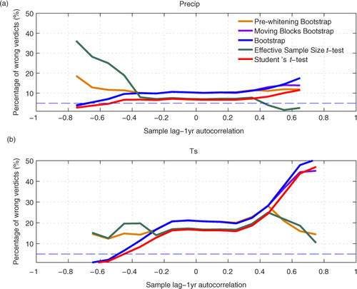
Fig. 3 Performance of the five statistical techniques in establishing the robustness of 20-yr average. Percentage of wrong verdicts refers to the probability of confidence interval not containing the truth. Since two-tailed significance tests were conducted at a 5% significance level, the correct percentage of wrong verdicts should be 5% (marked with dashed line). Autocorrelation here is the lag-1 yr autocorrelation measured in a 20-yr continuous simulation.

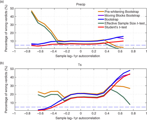
In Fig. 3, the performance of the techniques is measured by the percentage of wrong verdicts, which should approach 5% when the technique works correctly. The percentage of wrong verdicts varies widely from near 0 to 50%, which casts doubt on the overall performance of statistical techniques. The performance is reasonably good for precipitation when the autocorrelation is weak. However, for Ts, the performance is not so good for most autocorrelations. At near zero autocorrelations, the derived 95% confidence intervals are actually 80~85% intervals. The performance difference between Ts and precipitation is very interesting, and the investigations for the reasons are in the next section.

Focussing on the performance difference between techniques, Student's t-test, the moving blocks bootstrap test and bootstrap test show very similar performance, while Student's t-test systematically outperforms the other two techniques by a small margin. Thus, we do not see any good reason to apply the other two techniques in climate model simulation. The pre-whitening bootstrap test and the effective sample size t-test show similar performance, while the latter outperforms the former. In this regard, the pre-whitening bootstrap test does not have grounds in climate simulation. Between the effective sample size t-test and Student's t-test, the former outperforms the latter when autocorrelation is positive and strong (>+0.6) and Ts is analysed. Even with strong positive autocorrelation, the effective sample size t-test does not particularly outperform Student's t-test when analysing precipitation, as it tends to give too wide confidence intervals in this case. In strong negative autocorrelation cases, Student's t-test performs better in both Ts and precip by a big margin. Overall, we find that Student's t-test performs at least as well as the other four techniques.

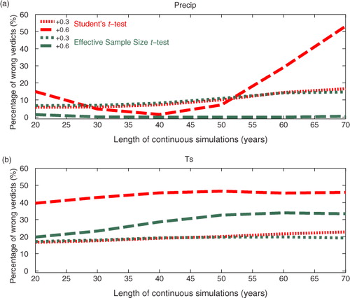
Our conclusion is that there is no reason to replace Student's t-test by the advanced techniques in most cases. This conclusion is based on the analysis of 20-yr averages. The technique performances are found to be qualitatively similar even if we analyse longer than 20 yr averages. Figure 4 demonstrates this by comparing the effective sample size t-test to Student's t-test for 20~70-yr long samples. Thus, our conclusion is insensitive to the length of climate model run. Note that the results with lag-1 yr autocorrelations of +0.6 (Fig. 4a) are not robust because such strongly autocorrelated cases become very rare for precipitation when the length of the sample increases.

Fig. 4 Same as Fig. 3, except that the performance of the Student's t-test and the Effective Sample Size t-test is shown as a function of the integration length of the continuous simulation. In Fig. 3, only 20-yr long runs were analysed. Red curves correspond to Student's t-test, and green curves correspond to the Effective Sample Size t-test. The two curves of the same colour represent weak positive (+0.3) and strong positive (+0.6) lag-1 yr autocorrelations in the 20~70 yr long continuous simulation.

When autocorrelation is very strong and positive (>+0.6), the effective sample size t-test is better than or as good as Student's t-test (Fig. 3). As Figs. 1 and 2 show, +0.6 or greater autocorrelation is almost non-existent in precipitation while it is present but rare in Ts. The area of strongly positive autocorrelation is limited to minor portions of the extratropics in fully coupled models (Fig. 1). Autocorrelation tends to be more strongly positive in the extratropics than the tropics (Fig. 1), probably because the extratropics is dominated by low-frequency variabilities associated with slow variations in ocean circulation. Figure 1also shows salient differences between the two fully coupled models in autocorrelation structures. In CESM1, autocorrelation is mainly positive everywhere, whereas the autocorrelation in ECHO-G is characterised by negative values in the tropics and positive values in the extratropics. We also look at other seasons and find similar features. This difference between CESM1 and ECHO-G is probably attributed to the way ENSO is simulated. If ENSO exhibits a strong biennial cycle, the autocorrelation would be negative. On the other hand, if ENSO is mostly governed by 4~5 yr of cycle, the autocorrelation would be positive.

4. Discussions

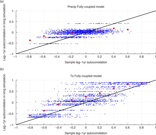
Previously, we demonstrated that the advanced techniques do not work better than Student's t-test overall. Out of these advanced techniques, three techniques account for autocorrelation: the effective sample size t-test, the moving blocks bootstrap test and the pre-whitening bootstrap test. We first investigate if the poor performance of these three techniques is because a 20-yr run (to which the techniques were applied) does not represent the long simulation well in terms of autocorrelation. Figure 5 does show that 20-yr runs do not match the long simulation very well. For instance, when a long simulation of Ts has a lag-1 yr autocorrelation of +0.5, 20-yr simulations extracted from this simulation have lag-1 yr autocorrelations of −0.3 to +0.4 (ignoring top 5% extremes), which indicates high variability of the autocorrelation in 20-yr runs. In addition, Fig. 5b shows that for Ts the autocorrelation in 20-yr runs is systematically lower (or more negative in case of negative values) than the autocorrelation in the long simulations. This sampling bias is nearly constant for most of the autocorrelations in the long simulations. For precipitation however, lag-1 yr autocorrelation in the long simulations tends to be amplified in 20-yr runs (Fig. 5a).

Fig. 5 Scatter plot of lag-1 yr autocorrelation in 20-yr long continuous simulations against lag-1 yr autocorrelation in long simulations. Time series of area averages from climate models, as explained in Section 2, are used. Note that red dots are shown to denote the averages for the lag-1 yr autocorrelation in long simulations as a function of the sample 1ag-1 yr autocorrelation; the results are obtained by binning the data at intervals of 0.2 in sample 1ag-1 yr autocorrelation.

In Fig. 6, we evaluate the performance of the significance tests as in Fig. 3, except that the autocorrelation in the long simulation is used instead of that in a 20-yr run. Since Student's t-test and the bootstrap test do not account for autocorrelation, the performance for these two techniques remains unchanged. In the autocorrelation adjusting techniques, the moving blocks bootstrap test and the effective sample size t-test are found to be not strongly affected by this autocorrelation substitution experiment. The performance of the pre-whitening bootstrap test is somewhat enhanced in this experiment. This is most likely due to the sensitivity of the technique to the quality of the pre-whitening (Efron and Tibshirani, 1993), i.e. autocorrelation filtering. Optimal pre-whitening is achieved when nearly uncorrelated residuals remain after pre-whitening. Using the autocorrelation of the 20-yr run will yield more correlated residuals due to the uncertainty on the autocorrelation in short runs. This will in turn affect the subsequent procedure of the technique application (see Appendix). Overall, we can conclude from the autocorrelation substitution experiment that autocorrelation adjustment in the advanced techniques can be made using the autocorrelation information within the tested 20-yr run without severely affecting the technique performance.

Fig. 6 Same as Fig. 3, except that the advanced techniques use the autocorrelation from the long simulation for the autocorrelation adjustments instead of using the autocorrelation in the 20-yr long sample.

Then, why do the advanced techniques perform poorly relative to Student's t-test? We also looked into multiple-year lag autocorrelations instead of just lag-1 yr autocorrelation, but failed to provide a convincing explanation. It is our hope that the findings presented in this study will stimulate future studies so as to better understand the poor performance. Real climate data exhibit various features that autocorrelation alone cannot fully explain. For instance, there is strong asymmetry between positive and negative anomalies in the data, and linear measures such as autocorrelation are unable to address the asymmetry.

In the previous section, we also noted a significant performance difference between Ts and precipitation in Fig. 3. Ts shows more low-frequency variability than precipitation. This is reflected in lag-1 yr autocorrelation, in that strong positive autocorrelation is more common in Ts than in precipitation (Fig. 3). Observed temperatures also exhibits long-term persistent behaviour on a decadal or centennial time scale (Koscielny-Bunde et al., 1998; Fraedrich and Blender, 2003; Vyushin et al., 2004). When we select subsets of the time series in Ts that are equal to those in precipitation in terms of both short-term persistence (quantified by lag-1 yr autocorrelation) and long-term persistence (quantified by multiple-year lag autocorrelation), the noted performance difference between Ts and precipitation disappears. Thus, we conclude that long-term persistence makes significance techniques to work poorly.

5. Conclusions

In this study, we have measured the performance of Student's t-test and four advanced statistical techniques in conducting two-tailed significance tests on 20-yr continuous simulations. Although the advanced techniques were developed to improve upon Student's t-test, we find that these advanced techniques underperform Student's t-test in most cases. A sizable performance gain using two of the advanced techniques over Student's t-test is limited to the model output portion with strong positive sample lag-1 yr autocorrelation (>+0.6). This gain is not consistent, in that Ts shows the gain and precipitation does not. Thus, the modellers would benefit from using some of the advanced techniques, after making sure that the autocorrelation in the obtained 20 yr of run is strongly positive and the variable for analysis would benefit. In reality, climate modellers do not check either. In rare cases where climate modellers apply an advanced technique, they usually do so without checking these aspects. Given these typical climate model output processing tendencies by modellers, we do not see a reason to replace Student's t-test by the advanced techniques.

Acknowledgements

This work was supported by the Korea Meteorological Administration Research and Development Program (ref: CATER 2012-7100) and by the Korean-Sweden Research Cooperation Program of the National Research Foundation of Korea (ref: 2012K2A3A1035889). We furthermore acknowledge the Model and Data Group at Max Planck Institut für Meteorologie for making their ECHO-G output available for analysis. Special thanks to Eduardo Zorita of the Helmholtz-Zentrum Geesthacht for pointing us to this data.

7. Appendix: Description of the five statistical techniques

A1. Student's t-test

In Student's t-test the observed test statistic is the signal-to-noise ratio, known as t-value. It is calculated asA1

where represents the average of a sample of size n, µ is the hypothesised mean of the population, and the Standard Error of the Mean (SEM), a measure for noise, is given byA2

where s is the sample standard deviation. For a one-sample t-test, the signal is the difference between the sample average and the hypothesised population mean. In case the goal is to test if two model simulations are significantly different, i.e. a two-samples t-test, SEM is a combination of SEMs from both simulations and the signal is the difference of the averages of the two simulations.

The t-value (eq. A1) is a standardised test statistic and must be compared with standardised distributions, namely the t-distributions: William Sealy Gosset (who published his work under the pen name Student) found that for small samples drawn from a normal distribution, the sampling distribution follows a bell-shaped distribution that deviates from the normal distribution (for larger sample sizes, the sampling distribution converges to a normal distribution). He called those distributions the t-distributions and found that the shape depends on the sample size n. To find the t-distribution that represents the sampling distribution the best, the degrees of freedom ν is calculated using eq. (A3).A3

More complicated equations exist for the degrees of freedom. For instance, in a two-sample t-test where the variance in both samples is different, the degrees of freedom must be calculated with a more complicated formula.

Once the best fitting t-distribution is found, confidence intervals (CIs) can be calculated withA4

where t _crit is the t-value that denotes the critical region of H ₀ rejection on a standardised t-distribution defined by the degrees of freedom ν. t _crit values are tabulated or calculated from the cumulative t-distribution function.

A2. The effective sample size t-test

This test is a modified version of Student's t-test in which a correction is introduced for samples with autocorrelated values. When elements (or values) in a sample are not independent, the effective amount of data available for statistical inference is not the same as would be initially expected. Consequently, SEM will be wrongly estimated. It is proposed to replace n by n _eff , where n _eff is the number of effectively independent values in the sample, estimated asA5

withA6

where the theoretical autocorrelation coefficient ρ_τ is given byA7

for

where K is the order of the autoregressive (AR) process which is fitted to the sample and the φ _k are the autoregressive parameters of the AR process. τ represents the lags in the sample. For instance, if the sample is a monthly time series, τ ranges from 1 month to K months. The best order K of the AR model to fit the sample can be found using a goodness-of-fit statistic such as the Bayesian Information Criterion (Schwarz, 1978) or the Akaike Information Criterion (Akaike, 1974), both of which are described in Section A6. The autoregressive parameters φ _k can be estimated using the Yule-Walker equations:A8

where r _K are the lag-K-correlation coefficients measured in the sample.

The remainder of the effective sample size t-test is the same as Student's t-test.

For more information on the effective sample size t-test, see (Wilks, 1997Wilks, 2011) and (Zwiers and Von Storch, 1995).

A3. The bootstrap test

Student's t-test is a parametric test, which means that an assumption about the distribution of the population is made. For Student's t-test, the population is assumed to follow a normal distribution. Non-parametric tests do not make any assumptions about the shape of the population distribution. The bootstrap test is such a non-parametric test. To obtain the sampling distribution, the available sample is resampled numerous times (typically thousands of times). The resampling method is analogous to a lottery. Say each lottery ticket contains a single value of the sample of size n. The n lottery tickets are thrown into a container and well mixed. Lottery tickets are drawn one by one, but after each draw, the tickets are replaced in the container. Some values may be drawn several times. Enough lottery tickets are drawn so that new samples of size n are ‘created’ from the original sample. For each new sample thus created, the statistic of interest is computed, e.g. the sample average. Thus, a reasonable approximation of the sampling distribution of that statistic is empirically constructed. The critical region of rejection can be determined on this empirical sampling distribution. Usually, this is sufficient to draw a conclusion about a stated hypothesis. If the interest is to construct CIs, they can be derived from the empirical cumulative distribution using the so-called percentile method. These CIs may have to be corrected, especially for small sample sizes (Efron and Tibshirani, 1993). Different methods exist to correct these confidence intervals, such as the normal CIs, the corrected percentile CIs, the studentised CIs or the BCa CIs, to mention just a few of the methods available. In this paper, we have used the percentile CIs without correction as the above-mentioned corrections were not found to significantly improve on the performance of the significance tests shown in Fig. 3.

The bootstrap test (Efron, 1982; Efron and Tibshirani, 1993) is a relatively recent technique known for its versatility, meaning that the sampling distribution of any test statistic can be estimated easily, not just the average of a sample.

A4. The moving blocks bootstrap test

The moving blocks bootstrap test is a modification of the bootstrap test in case dependence in the sample exists. The resampling technique from the bootstrap test tends to destroy autocorrelation patterns. However, if the resampling procedure is done in blocks of certain length in the sample (meaning the order in which values appear in the sample is not changed), parts of the autocorrelation patterns are retained. The difficulty consists in choosing the length of the blocks. Too long blocks will not give sufficiently diverse samples and the resulting sampling distribution will not be representative enough of the real sampling distribution. Too short blocks will disrupt autocorrelation patterns leading to a wrong estimation of the sampling distribution. Wilks (1997) optimised the calculation of the block length for samples that can be assumed to follow an autoregressive model (AR) (other equations to calculate the block length exist, e.g. as described by Künsch, 1989).

If the order of the AR model is 1, the formula for the block length is given by:A10

WithA11

If the order of the AR model is 2, the formula for the block length is given by:A12

WithA13

V in eqs. (A11) and (A13) is found using eq. (A6). In this study, we assumed eqs. (A12) and (A13) are also applicable on the samples fitting higher order AR models. The vast majority of the samples were categorised as best fitted with an AR1 or AR2 model. Only an insignificant fraction of the samples were fitted with higher order AR models (3 or 4). The best order of the AR model to fit the sample can be found using a goodness-of-fit statistic such as the Bayesian Information Criterion (Schwarz, 1978) or the Akaike Information Criterion (Akaike, 1974), both of which are described in Section A6.

A5. The pre-whitening bootstrap test

This test is an alternative to the moving blocks bootstrap test. The main idea is to filter out or ‘pre-whiten’ any dependency found in the sample to obtain noise residues. These residues are bootstrapped with the classic bootstrap test. Afterwards, a new sample is reconstructed by adding back the filtered structures to the bootstrapped residues. On each new sample thus created the test statistic of that sample is calculated. The complication resides in a good filtering technique to obtain the noise residues. If the data in the original sample can be well-fitted to a time series model, it is possible to isolate the dependent features from independent residues. The residues are ideally normally distributed white noise. Box and Jenkins (1976) developed a well-established fitting methodology, but the methodology is not straightforward (Wilks, 2011) and requires trial fittings and subsequent goodness-of-fit statistics (see Section A6 below) in order to find the optimal AR model to fit the data. In this paper, we only fitted samples to AR models, as is most commonly done. A more detailed description of the pre-whitening bootstrap test is given by Solow (1985) and Efron and Tibshirani (1993).

A6. Order selection criteria

For the effective sample size t-test, the moving bootstrap test and the pre-whitening bootstrap test, the samples must be fitted to a certain AR model. The order of this AR model is important to calculate the noise estimation adjustment. When a sample is overfitted, i.e. fitted to an AR with a too high order, too many terms will be added to the noise estimation correction [e.g. in eq. (A6)] resulting in wrong noise estimations (Wilks, 2011). The usual way to find the best fitting order is to use the Bayesian Information Criterion (BIC) (Schwarz, 1978) or Akaike Information Criterion (AIC) (Akaike, 1974).A14 A15

with K the order of the model to test and is the variance of the residual noise after fitting the sample to the AR model of order K. This variance term can be calculated from the residual noise terms ɛ _τ from the equation for AR model of order K:A16

where x _{τ + 1} is the value at the next time lag τ + 1, µ is the average of the time series, K is the order of the model, φ _k is the autoregressive coefficient that must be found with eq. (A8) and ɛ _{τ + 1} is the noise residual at the next time lag τ + 1. Note that the collection of residuals ɛ _τ is assumed to be normally distributed white noise. ɛ ₁ is usually assumed to be 0 or µ.

Once the BIC or AIC are calculated for several candidate orders K, the BIC or AIC with the smallest value denotes the order K of the AR model that will best fit the sample.

References

- Akaike H . A new look at the statistical model identification. IEEE Trans. Automat. Contr. 1974; 19: 716–723.
- Box G. E. P , Jenkins G. M . Time Series Analysis: Forecasting and Control. 1976; Ann Arbor, MI, USA: Holden-Day, the University of Michigan. 575.
- Chung C. E , Ramanathan V , Kiehl J. T . Effects of the South Asian absorbing haze on the northeast monsoon and surface – air heat exchange. J. Clim. 2002; 15: 2462–2476.
- Collins W. D , Rasch P. J , Boville B. A , Hack J. J , McCaa J. R , co-authors . The formulation and atmospheric simulation of the Community Atmosphere Model Version 3 (CAM3). J. Clim. 2006; 19: 2144–2161.
- Efron B . The Jackknife, the Bootstrap, and Other Resampling Plans. 1982; Philadelphia, PA, USA: Society for Industrial Mathematics. 92.
- Efron B , Tibshirani R. J . An Introduction to the Bootstrap. 1993; New York, NY, USA: Chapman and Hall. 436.
- Elmore K. L , Baldwin M. E , Schultz D. M . Field significance revisited: spatial bias errors in forecasts as applied to the Eta Model. Mon. Weather Rev. 2006; 134: 519–531.
- Fraedrich K , Blender R . Scaling of atmosphere and ocean temperature correlations in observations and climate models. Phys. Rev. Lett. 2003; 90: 108501.
- Gent P. R , Danabasoglu G , Donner L. J , Holland M. M , Hunke E. C , co-authors . The Community Climate System Model Version 4. J. Clim. 2011; 24: 4973–4991.
- Jin C. S , Ho C. H , Kim J. H , Lee D. K , Cha D. H , co-authors . Critical role of northern off-equatorial sea surface temperature forcing associated with central pacific el Niño in more frequent tropical cyclone movements toward East Asia. J. Clim. 2013; 26: 2534–2545.
- Koscielny-Bunde E , Bunde A , Havlin S , Roman H. E , Goldreich Y , co-authors . Indication of a universal persistence law governing atmospheric variability. Phys. Rev. Lett. 1998; 81: 729–732.
- Kunkel K. E , Liang X. Z , Zhu J . Regional climate model projections and uncertainties of U.S. summer heat waves. J. Clim. 2010; 23: 4447–4458.
- Künsch H. R . The Jackknife and the Bootstrap for general stationary observations. Ann. Stat. 1989; 17: 25.
- Lee T , Ouarda T. B. M. J , Ousmane S , Moin S. M. A . Predictability of climate indices with time series models. Stochastic Hydrology of the Great Lakes – A Systemic Analysis.
- Roeckner E , Bäuml G , Bonaventura L , Brokopf R , Esch M . The atmospheric general circulation model ECHAM 5. PART I: model description. 2003; Hamburg, Germany: Max-Planck-Institut für Meteorologie.
- Schwarz G . Estimating the dimension of a model. Ann. Stat. 1978; 6: 4.
- Solow R. A . Bootstrapping correlated data. J. Int. Assoc. Math. Geol. 1985; 17: 769–775.
- Soltani S , Modarres R , Eslamian S. S . The use of time series modeling for the determination of rainfall climates of Iran. Int. J. Clim. 2007; 27: 819–829.
- Von Storch H , Zwiers F. W . Statistical Analysis in Climate Research. 1999; Cambridge, UK: Cambridge University Press. 484.
- Vyushin D , Zhidkov I , Havlin S , Bunde A , Brenner S . Volcanic forcing improves atmosphere-ocean coupled general circulation model scaling performance. Geophys. Res. Lett. 2004; 31: L10206.
- Wei J , Dirmeyer P. A , Guo Z , Zhang L , Misra V . How much do different land models matter for climate simulation? Part I: climatology and variability. J. Clim. 2010; 23: 3120–3134.
- Wilks D. S . Resampling hypothesis tests for autocorrelated fields. J. Clim. 1997; 10: 65–82.
- Wilks D. S . Statistical Methods in the Atmospheric Sciences. 2011; Elsevier, Waltham, MA, USA: Academic Press. 676.
- Zorita E , González-Rouco F , Legutke S . Testing the Mannetal. (1998) Approach to paleoclimate reconstructions in the context of a 1000-Yr control simulation with the ECHO-G coupled climate model. J. Clim. 2003; 16: 1378–1390.
- Zwiers F. W . Statistical considerations for climate experiments. Part II: multivariate tests. J. Clim. Appl. Meteorol. 1987; 26: 477–487.
- Zwiers F. W , Thiébaux H. J . Statistical considerations for climate experiments. Part I: scalar tests. J. Clim. Appl. Meteorol. 1987; 26: 464–476.
- Zwiers F. W , Von Storch H . Regime-dependent autoregressive time series modeling of the Southern Oscillation. J. Clim. 1990; 3: 1347–1363.
- Zwiers F. W , Von Storch H . Taking serial correlation into account in tests of the mean. J. Clim. 1995; 8: 336–351.