Comparison of calculated energy flux of internal tides with microstructure measurements

Abstract

Vertical mixing caused by breaking of internal tides plays a major role in maintaining the deep-ocean stratification. This study compares observations of dissipation from microstructure measurements to calculations of the vertical energy flux from barotropic to internal tides, taking into account the temporal variation due to the spring-neap tidal cycle. The dissipation data originate from two surveys in the Brazil Basin Tracer Release Experiment (BBTRE), and one over the LArval Dispersal along the Deep East Pacific Rise (LADDER3), supplemented with a few stations above the North-Atlantic Ridge (GRAVILUCK) and in the western Pacific (IZU). A good correlation is found between logarithmic values of energy flux and local dissipation in BBTRE, suggesting that the theory is able to predict energy fluxes. For the LADDER3, the local dissipation is much smaller than the calculated energy flux, which is very likely due to the different topographic features of BBTRE and LADDER3. The East Pacific Rise consists of a few isolated seamounts, so that most of the internal wave energy can radiate away from the generation site, whereas the Brazil Basin is characterised by extended rough bathymetry, leading to a more local dissipation. The results from all four field surveys support the general conclusion that the fraction of the internal-tide energy flux that is dissipated locally is very different in different regions.

• Internal tides
• microstructure measurement
• vertical mixing

1. Introduction

Ocean circulation is primarily driven mechanically by wind-stress at the ocean surface and vertical mixing in the interior (Munk and Wunsch, 1998). The latter is caused by breaking of internal waves, and in the deep ocean such waves are mainly excited by tidal currents flowing over rough bottom topography (St. Laurent and Garrett, 2002). Inverse calculations using satellite altimetry data have confirmed that significant conversion from barotropic to internal tides takes place in the deep ocean and in the vicinity of large steep topographic features (Egbert and Ray, 2001, 2002). The vertical mixing caused by these internal tides plays an essential role in maintaining the stratification in the deep ocean, and hence in controlling the thermohaline circulation (Samelson, 1998; Zhang et al., 1999; Wunsch and Ferrari, 2004; Garrett and Kunze, 2007).

Observational programs conducted during the Brazil Basin Tracer Release Experiment (hereafter BBTRE) convincingly showed that vertical turbulent diffusivity is greatly enhanced over the rough Mid-Atlantic Ridge bottom topography, implying a connection between the deep-ocean mixing and the underlying bathymetric roughness (Polzin et al., 1997; Ledwell et al., 2000; St. Laurent et al., 2001). The enhanced turbulent dissipation inferred from these observations, which is likely caused by breaking of internal tides (Ledwell et al., 2000; Toole, 2007), has provided the motivation for many studies on the generation and dissipation of these waves (e.g. Polzin, 2004, 2009; Muller and Bühler, 2009; Nikurashin and Legg, 2011). The field survey results obtained during the LArval Dispersal along the Deep East Pacific Rise (hereafter LADDER) project provides additional evidence for a connection between bottom topography, internal waves and turbulent mixing from a different region. In particular, over the East Pacific Rise crest and flanks, turbulence levels were found to vary with the spring-neap tidal cycle on short time scales (Thurnherr and St. Laurent, 2011), whereas the modulation of internal wave levels (as well as parameterised turbulent mixing) on longer time scales was found to be dominated by subinertial flows, including those of mesoscale eddies (Liang and Thurnherr, 2012). The importance of cross-sill flows for the mixing was also enhanced during the GRAVILUCK cruise over the Mid-Atlantic Ridge (St. Laurent and Thurnherr, 2007).

Other mechanisms than internal tides can also contribute to enhanced mixing over rough bottom topography, such as overflow-related processes in the ridge-flank canyons of the Mid-Atlantic Ridge (Thurnherr et al., 2005), or the generation of internal waves through the interaction of geostrophic eddies with rough small-scale bottom topography (Nikurashin and Ferrari, 2010a, 2010b).

Nycander (2005) used a method based on linear wave theory developed by Bell (1975a, 1975b) and Llewellyn Smith and Young (2002) to calculate the global distribution of the energy conversion from barotropic to internal tides for the eight major tidal constituents. The input data needed for his global computation are the bottom topography, the tidal-velocity field, and the stratification of the ocean. He predicted the generated internal-tide energy to be two orders of magnitude larger over the rough bottom topography of the Mid-Atlantic Ridge than over the extended plain in the western part of the Brazil Basin, in qualitative agreement with BBTRE measurements of turbulent energy dissipation (Polzin et al., 1997).

There are several limitations to the computation by Nycander (2005): (1) it is not valid when the slope is supercritical, although a correction for supercritical slopes has recently been proposed by Melet et al. (2013), (2) it uses the WKB approximation, which simplifies the treatment of non-uniform stratification, and (3) small-scale topographic features are generally not well resolved in currently available topographic datasets. In spite of these limitations, some support for the validity of Nycander's approach (2005) is given by the results of Green and Nycander (2013), who used this scheme to parameterise the wave drag in a prognostic tidal model. They found that the parameterisation substantially improved the performance of the tidal model compared to two other parameterisations based on simple scaling arguments.

Melet et al. (2013) have used Nycander's method to assess the effect of small-scale abyssal hills on estimates of the energy flux of the M ₂ internal tide. These small-scale features are not resolved in the global bathymetry dataset, and were therefore synthetically generated and added to the dataset. Using an empirical correction for supercritical slopes, they also tried to quantify the overestimate of the energy flux of the M ₂ internal tide predicted by linear wave theory for supercritical slopes. Taking into account the abyssal hills, Melet et al. (2013) found a 10% increase in the global energy conversion rate, and up to 89% in a region in the Brazil Basin. Melet et al. (2013) did not compare their results to measurement.

The objective of the present study is to undertake a detailed comparison between the computed vertical energy flux of internal tides and observed energy dissipation rates from the microstructure measurements. We calculate the vertical energy flux by adopting an approach similar to Nycander (2005), but extended to predict the time variability of local turbulent dissipation due to the spring-neap tidal cycle. We compare these estimates to the dissipation rates measured during the BBTRE, LADDER3, and GRAVILUCK field surveys, as well as those obtained near the Izu-Ogasawara Ridge. We also examine the sensitivity of the calculated energy flux to spatial and temporal smoothing, as well as to the bathymetry resolution. To assess the contribution of the supercritical slopes to the energy flux, we extend the empirical correction for supercritical slopes proposed by Melet et al. (2013) for the M ₂ internal tide, so that it applies to the eight major tidal constituents.

In Section 2, we present the method of calculation of vertical energy fluxes (complemented with Appendices A and B), the dissipation measurements and the methodology used to compare energy flux estimates with dissipation data. Results of the comparison of the energy flux with the observed energy dissipation data are presented in Section 3. Section 4 describes how the averaging of the calculated energy flux and the vertical integration of the energy dissipation were optimised. A summary and conclusion are given in Section 5.

2. Data and methods

2.1. Calculation of vertical energy flux

One of our objectives is to assess the time variability associated with observed depth-integrated energy dissipation from the microstructure measurement. Hence, the temporal behaviour of the vertical energy flux at the bottom needs to be calculated. The time-dependent vertical energy flux is defined as C≡pw, where p and w are the bottom pressure perturbation and vertical velocity resulting from the interaction of the barotropic tidal current with bottom topography, respectively. A time-independent expression of the vertical energy flux is also used, based on Nycander (2005).

A detailed derivation of the vertical energy flux is given in Appendices A and B. The calculations are based on linear wave theory (Llewellyn Smith and Young, 2002), which is valid for subcritical slopes (, where ω is the tidal frequency, N the buoyancy frequency, and f the Coriolis parameter). A further assumption made for the calculations is that the horizontal tidal excursion is small compared to the horizontal scale of the bottom topography, implying that the internal tide predominantly radiates at the tidal frequency. Finally, the calculations use the WKB approximation in the vertical direction. As a result, the vertical energy flux is proportional to the bottom buoyancy frequency N _B , instead of depending on the detailed structure of stratification profile. As shown by Zarroug et al. (2010), this is accurate for the high modes associated with small-scale topography, but less so for the lowest internal wave modes, which are associated with large-scale topography.

In order to construct a time series of energy flux, data sets of ocean bathymetry, barotropic tidal velocity and buoyancy frequency are required. For the bottom topography, we used the GEBCO (General Bathymetric Chart of the Oceans) global 30 arc-second gridded dataset. The sensitivity of the vertical energy flux to the topographic dataset was assessed through the comparison with the results obtained using the ETOPO2v2 2-minutes Gridded Global Relief dataset (available online at http://www.ngdc.noaa.gov/mgg/global/etopo2.html).

Barotropic tidal velocities were extracted from the TPXO6.2 model (Egbert and Erofeeva, 2002) with a resolution of 1/4° and then interpolated onto the topographic grid. The eight major tidal components (M ₂, S ₂, N ₂, K ₂, K ₁, Q ₁, P ₁, O ₁) were used to compute the energy flux, thus capturing the spring-neap cycle of tidal forcing, which is mainly due to interference between M ₂ and S ₂.

The buoyancy frequency N was calculated from the WOCE Global Hydrographic Climatology (WGHC, Gouretski and Koltermann, 2004) with a 1° horizontal resolution and 45 vertical levels. The climatology was linearly interpolated onto the topographic grid points, and the buoyancy frequency of the deepest vertical level above the bathymetry was then chosen as the bottom buoyancy frequency N _B .

2.2. Observations of turbulent dissipation

The observational estimates of the energy dissipation rate were based on microstructure measurements. They can be made using a so-called High Resolution Profiler (HRP). A HRP is a free-falling instrument sampling temperature, salinity and horizontal velocity profiles at high vertical resolution (~1 mm) (Toole et al., 1997). HRP measurements are sufficiently well resolved to provide accurate estimates of instantaneous turbulent-kinetic-energy dissipation rates.

During the two BBTRE surveys carried out in 1996 and 1997, microstructure measurements were made using HRPs to examine the diapycnal mixing in the Brazil Basin (Montgomery, 1998). In the February–March 1996 survey, hereafter BBTRE1, a total of 72 valid full-depth HRP profiles were collected (Fig. 1a). The main purpose of BBTRE1 was to investigate the difference between the turbulent dissipation rates in the western Brazil Basin with a relatively smooth bathymetry and those at the Mid-Atlantic Ridge featuring a network of rough fracture zones. During the March–April 1997 survey, henceforth denoted BBTRE2, 88 full-depth microstructure measurements were conducted, focusing on a detailed sampling of the Mid-Atlantic Ridge (Fig. 1a). Thus, a total of 160 HRP profiles were successfully obtained during the two BBTRE surveys. The microstructure data from both surveys have been discussed and analysed by Polzin et al. (1997), St. Laurent et al. (2001), Polzin (2004), Thurnherr et al. (2005), and Toole (2007).

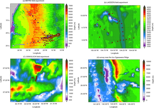
Fig. 1 (a) The locations of 75 stations during the BBTRE1 field experiment (blue circles) and those of 90 stations during the BBTRE2 field experiment (red circles). The cross-marked circles indicate the stations which are excluded in the analysis in this paper. (b) The locations of 37 stations during the LADDER3 field experiment. (c) The locations of 12 stations occupied in the GRAVILUCK field experiment. (d) The locations of 10 stations near the Izu-Ogasawara Ridge.

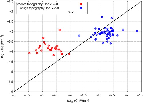
The distance between the seabed and the lowest observation point is typically a few tens of meters, although it varies depending on the stations. A large amount of dissipation usually occurs near the ocean bottom, so we decided to consider only stations where the deepest observation point is less than 150 m from the ocean bottom. For this reason, we excluded four stations from BBTRE1 and three stations from BBTRE2. In addition, we excluded 24 stations of BBTRE1 located in the Brazil Basin west of 28°W, because the calculated vertical energy flux is too small to explain the observations. West of 28°W the Brazil Basin is characterised by the smooth bathymetry of an abyssal plain, resulting in very weak internal tides. This is seen in Fig. 2, which shows a scatter plot of the vertical energy flux averaged over the final 72 hours of the time series versus the observed energy dissipation rate integrated over the depth range 50 m to 2000 m above the bottom topography. Apparently, most of the dissipation west of 28°W is not caused by locally generated internal tides, and instead might relate to some background turbulent dissipation field. There is of course no point in correlating the energy flux and the local dissipation in this region, and these stations are therefore excluded. As a result, a total of 127 BBTRE stations (43 HRP stations from BBTRE1 and 84 stations from BBTRE2) were retained for the subsequent analysis. The total ocean depths at these selected stations are in the range 3857<H<5593 m, with an average depth of 4640 m.

Fig. 2 Logarithmic scatter plot of the energy dissipation ɛ integrated up to 2000 m above the bottom, D, versus averages of the last 72 hours of vertical energy flux C=pw from model predictions. The weighted average of C at the observational sites is obtained from all the grid points within the radius γ. The diagram comprises 75 stations from the BBTRE1 survey, coloured according to the longitude of the observational site, so that the blue and red circles are the sites east and west of the longitude −28°, respectively.

We also considered microstructure profiles sampled during the LADDER3 survey (Fig. 1b), obtained with an instrument similar to HRP called deep microstructure profiler (Thurnherr and St. Laurent, 2011). LADDER3 was conducted near the crest of the East Pacific Rise (EPR), between 9°30′N and 10°N, during November and December 2007. Of the 37 microstructure profiles obtained during LADDER3, we used 26 profiles that reached within 150 m from the ocean bottom. The total ocean depths at the 26 selected stations are in the range 1700<H<3135 m, with an average depth of 2600 m.

We also considered 12 deep microstructure profiles from the GRAVILUCK cruise (Fig. 1c), carried out in the Mid-Atlantic-Ridge Lucky Strike segment at 37°N in August 2006 (St. Laurent and Thurnherr, 2007). All 12 considered profiles from this cruise reached within 150 m from the bottom. The total ocean depths at these stations are in the range 1870<H<2770 m, with an average depth of 2100 m. Finally, 10 microstructure profiles sampled near the Izu-Ogasawara Ridge in the west Pacific were analysed (hereafter IZU, Fig. 1d), including seven profiles sampled in November 2008 and 3 in December 2011 (Hibiya et al., 2012). The total ocean depths at these stations are in the range 3036<H<4932 m, with an average depth of 4023 m. All the 10 considered profiles from IZU reached within 200 m from the bottom. Given the small number of GRAVILUCK and IZU profiles, these data are not used in the main statistical analysis, but used to compare the magnitude of the theoretical prediction of the energy flux with the vertically integrated energy dissipation rate.

2.3. Comparison between energy flux and local dissipation

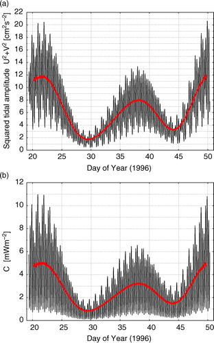
Our goal is to compare the calculated vertical energy flux associated with internal tides to the observational estimates of the vertically integrated energy dissipation rate. At each station, we first constructed a time series of instantaneous vertical energy flux, calculated with a temporal resolution of 1/2 hour, for 1 month prior to the observation. Figure 3 illustrates the time series of the energy flux, C=pw, obtained at a typical BBTRE1 station (station 64). Note the apparent cycle with a period approximately equal to 6.2 hours. This is because the vertical energy flux is quadratic in the barotropic tidal amplitude. On longer time scales, the time series features the spring-neap tidal cycle (2 weeks period) resulting mainly from the superposition of M ₂ and S ₂ tidal constituents.

Fig. 3 (a) Time series of the squared barotropic-tide amplitude at station 64 from the BBTRE1 experiment in 1996. All the eight major tidal constituents have been taken into account to obtain the time series. (b) Time series of the energy flux C at this station when all the eight major tidal constituents have been taken into account. In both (a) and (b), the red solid lines show the 3-d running average of the time series.

Before making the comparison, the energy flux is averaged both horizontally and temporally, while the dissipation rate is integrated vertically. This results in three parameters to be specified: α (the horizontal averaging length normalised to the cutoff length), Δt (the time averaging interval), and ΔH (the vertical integration interval).

Horizontal averaging of the energy flux was performed using a Gaussian filter with an e-folding scale of αγM ₂/2, applied to all the model grid points located within a radius αγM ₂ around each observation point. Here, α is a dimensional coefficient, and γM ₂ is the cutoff length of the M ₂ tidal constituent, as defined by Nycander (2005),1

where H is the total ocean depth. γM ₂ is proportional to the horizontal wavelength of the first internal wave mode, and is typically a few tens of kilometres or less.

The vertical energy flux time series were also averaged in time such that2

where t _obs is the time of observation, and Δt the time averaging interval. Sensitivity tests were performed using time intervals varying from 6 hours to 1 month. For comparison, we also computed the time-independent energy flux C _∞ using the expression of Nycander (2005) (see Appendix B), which corresponds to the energy flux averaged over an infinitely long time period.

The dissipation rate measurements were integrated vertically at each station:3

where ΔH _o was set to a constant so as to make the different stations more comparable to one another. We used ΔH _o =50 m for BBTRE, GRAVILUCK, and IZU. For LADDER3, we chose ΔH _o =100 m, since most stations did not reach 50 m from the bottom. For the upper bound of the integral, we use several values of ΔH from 500 to 3500 m. An alternative approach was also tested, using fixed distances from the surface for the upper bound of the integral, but this systematically gave less satisfactory results.

To decide the optimal set of averaging parameters, we calculate the linear correlation coefficient r between the energy flux and the energy dissipation rate in logarithmic space,4

and the best-fit line,5

where6 7

where x and y correspond to log₁₀(C) and log₁₀(D), respectively, brackets denote the arithmetic mean, cov(x,y) is the covariance, and var(x)=cov(x,x) the variance. Note that a linear function fit in logarithmic space is equivalent to the power law scaling D=10 ^b C ^a .

3. Results

Here we present the results from a comparison between the calculated vertical energy flux C due to the internal tide and the depth-integrated energy dissipation rate D for the BBTRE, LADDER3, GRAVILUCK, and IZU surveys. The results are based on optimal values of the three averaging parameters, that is, ΔH, α, and Δt. As discussed in Section 4, these values are determined by maximising the correlation of the linear least-squares fit between log(D) and log(C) for BBTRE and LADDER3, the two surveys with the largest amount of data. The optimal values α=1 and Δt=72 hours are used for all the four field surveys. For BBTRE and IZU, an optimal value of ΔH=2500 m is used. For LADDER3 and GRAVILUCK, ΔH=1500 m is used.

3.1. Scatter plots based on optimal parameters

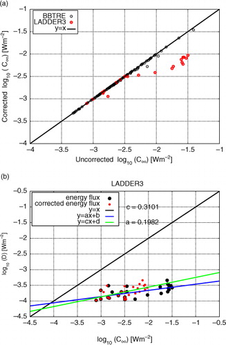
Figure 4a shows a scatter plot of the depth-integrated energy dissipation rate D versus the energy flux C for the 127 stations from the two BBTRE experiments, BBTRE1 and BBTRE2, using the optimal averaging parameters to be determined in Section 4. There is a good correlation between the logarithms of the observed integrated dissipation rate and the calculated energy flux. This is due to BBTRE2, as the calculated correlation for this survey is much higher than that for the BBTRE1 data. The slope of the best-fit line is smaller than unity, which is partly due to the uncertainty in the calculated flux, as explained in Appendix C. The integrated observed dissipation rates are on average smaller than the calculated energy fluxes, but of similar magnitude. In contrast, the LADDER3 experiment has integrated dissipation rates one to two orders of magnitude smaller than the calculated energy fluxes (Fig. 4b).

Fig. 4 (a) Logarithmic scatter plot of the energy dissipation rates ɛ integrated up to 2500 m above the ocean bottom versus the average of last 72 hours of the vertical energy flux C=pw for the 127 stations from the BBTRE1 and BBTRE2 experiments. The weighted average from all grid points within the radius γM ₂ is used to obtain C at the observational sites. (b) As in (a), but for 26 stations from the LADDER3 experiment. The energy dissipation rates ɛ are integrated up to 1500 m above the bottom. (c) As in (a), but for 12 stations from the GRAVILUCK experiment. The energy dissipation rates are ɛ integrated up to 1500 m above the bottom. (d) As in (a), but for 10 stations near the Izu-Ogasawara Ridge (IZU dataset). The energy dissipation rates ɛ are integrated up to 2500 m above the ocean bottom.

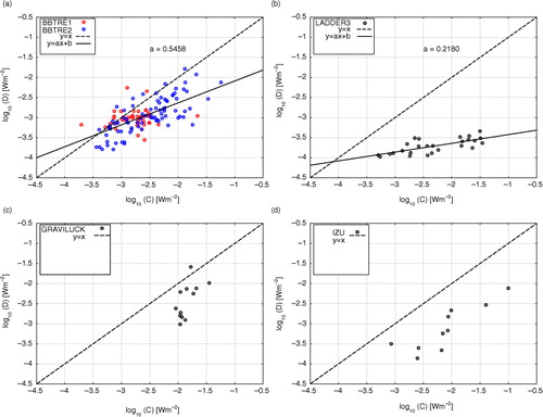
There are not enough profiles for the GRAVILUCK experiment to draw any conclusion about the correlation between integrated observed dissipation rates and energy flux, but we notice a substantial overlap between the GRAVILUCK and BBTRE scatter plots (Fig. 4c). In the IZU dataset, the depth-integrated dissipation is, on average, an order of magnitude smaller than the calculated energy flux. This is similar to the case of LADDER3, presumably because both were carried out near isolated topographic features. Such features, for example, the Hawaiian Ridge or the IZU Ridge, are more common in the Pacific Ocean than in the Atlantic, which is characterised by extended rough bottom topography. The correlations and the slopes of the fit-lines in Fig. 4 are summarised in Table 1.

Table 1. The optimal results of the statistical analysis carried out for BBTRE, LADDER3, GRAVILUCK and IZU datasets

Data set	r	a	p	d	d 10
BBTRE	0.66	0.5458	0.0000	0.35	0.85
LADDER3	0.71	0.2180	0.0049	0.02	0.20
GRAVILUCK	–	–	–	0.39	2.83
IZU	–	–	–	0.09	1.24

The correlation coefficient r, the slope a of the fit line, and the p values are listed. Also shown are the ratio between the vertically integrated dissipation and the energy flux, d, when the optimal height above the ocean bottom is used to vertically integrate the energy dissipation, and the corresponding ratio d ₁₀ when the energy dissipation is integrated vertically from the bottom to 10 m below the base of mixed layer. Note that d=0.05 for LADDER3 with correction for supercriticality.

3.2. Correction of energy flux for supercritical slope

Linear wave theory is not valid when the bathymetry slope is supercritical, and most likely overestimates the energy flux (see Appendix B). To remedy this, we use a simple method proposed by Melet et al. (2013). The correction is made only for the infinite temporal average of the energy flux C _∞ (see Appendix B), since applying it to the time-dependent C _Δt is impossible due to the interactions of tidal components.

In Fig. 5a, the corrected and uncorrected values of C _∞ are shown for BBTRE and LADDER3. For BBTRE, we can see that these two quantities are nearly identical for all the stations. Thus, the region in which BBTRE was carried out is mostly characterised by subcritical slopes. In contrast, C _∞ for the LADDER3 decreases up to a factor of 3 by this correction, especially at the seamounts with large energy flux (see Fig. 1b). Figure 5b shows scatter plots of the depth-integrated energy dissipation rates versus the energy flux obtained with or without the correction for supercritical slope. The values of the correlation coefficient r are 0.57 and 0.62 for the former and the latter cases, respectively, so that the empirical correction for supercritical slope rather reduces the correlation between C _∞ and D. On the other hand, the slope of the best-fit line increases from 0.2 to 0.3, although it is still much less than unity. More work remains to be done to better assess the validity of the proposed correction for supercritical slopes.

Fig. 5 (a) Logarithmic scatter plot of the corrected against the uncorrected values of the vertical energy flux C _∞ for 127 stations from the BBTRE experiment (black circles) and for 26 stations from the LADDER3 field survey (red circles). (b) Logarithmic scatter plot of the uncorrected C _∞ (black circles) and the corrected C _∞ (red circles) against the depth-integrated energy dissipation rate D for 26 stations from the LADDER3 field survey. The blue and green lines are the best-fit lines for the uncorrected C _∞ and the corrected C _∞, respectively.

3.3. Sensitivity to bathymetric data

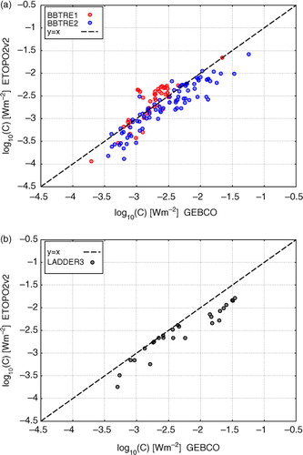
The vertical energy fluxes obtained using two different global topographic datasets (GEBCO and ETOPO2v2) are compared (see Fig. 6). At most of the stations for BBTRE and LADDER3, the vertical energy flux based on the GEBCO dataset is higher than that based on the ETOPO2v2 by a factor of about 2. There is also a rather large scatter of similar magnitude as the average difference. This can serve as a crude estimate of the uncertainty caused by the inaccuracy of the topography, and shows that higher resolution bathymetric products should be preferred for energy flux calculations.

Fig. 6 (a) Logarithmic scatter plot of 72-hours averages of the energy flux C obtained using bathymetry data from GEBCO and from ETOPO2v2. The diagram comprises 127 stations from the BBTRE experiment. A weighted average over the grid points within the radius γM ₂ is used to determine C at observational site. (b) As in (a), but for the 26 stations from the LADDER3 experiment.

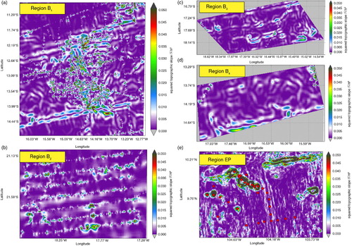
Topographic datasets such as GEBCO and ETOPO2v2 are derived from a combination of satellite altimetry and vessel-borne depth soundings. Since the latter have a sparse spatial coverage, the resolution of the topography is highly non-uniform. To illustrate this, we show plots of the squared bathymetric slope in GEBCO for the four selected regions in the Brazil Basin in Fig. 7a–d, as well as the region in the East Pacific where the LADDER3 field survey was conducted in Fig. 7e. The distance between the two successive annotations on the x−and y−axes is about 50 km in all these plots. Plotting the squared slope emphasises the small-scale features, and hereby shows where ship measurements have been used to construct the topographic data. Many such ship tracks are clearly seen in Fig. 7a and b. The same ship tracks can also be seen in plots of the energy flux to internal tides (not shown). The regions in Fig. 7c and d, on the other hand, are selected because they have very few ship tracks. These regions are typical for the topographic data in the region of the BBTRE surveys. As seen in Fig. 7e, the topography has a high resolution in the region of the LADDER3 survey, presumably because multibeam echosounder transects were available for this region.

Fig. 7 (a) The squared bathymetry slope calculated from the GEBCO data for the region B1 with many ship tracks. (b) As in (a), but for the rectangular region B2 with many ship tracks. (c) As in (a), but for the region B3 with very few ship tracks. (d) As in (a), but for the region B4 with very few ship tracks. (e) As in (a), but for the region EP where the LADDER3 field survey was conducted. The red circles represent the 37 stations during this field survey. Note that there is approximately 50 km between two successive tick marks on the axes in Figs. (a)–(e).

A comparison between Figs. 2 and 4b shows that the vertically integrated energy dissipation for LADDER3 is similar to the background values observed in the western part of the Brazil Basin, although the calculated energy flux resembles that in the eastern part of this Basin. The question arises why the discrepancy between the calculated energy flux and the observed dissipation rates becomes so large for LADDER3.

The calculated energy flux depends on the tidal forcing, the topographic slope, and the bottom stratification. To explore the possibility that the WOCE-derived bottom buoyancy frequency causes the above-mentioned discrepancy, we calculated the energy flux for LADDER3 using the buoyancy frequency near the bottom derived from the Thorpe-sorted hydrographic profiles (Thurnherr and St. Laurent, 2011). This yields very similar results (not shown) as those based on the WOCE-derived bottom stratification. Also, the discrepancy between the predicted energy flux and the observed dissipation is too large to be explained by errors in the tidal amplitude. A more likely explanation is that the employed bottom topography data, indeed, have a higher effective resolution in the LADDER3 case (Fig. 7e), which may have increased the calculated energy flux for LADDER3 as compared to BBTRE.

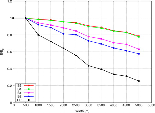
To understand the effects of the topographic resolution, we compare the calculated vertical energy flux in each of the four regions in the Brazil Basin, viz. B1, B2, B3 and B4 with that in the region EP (Fig. 7). Ten low-passed bathymetries are created by applying a boxcar filter with a width 500–5000 m with an increment of 500 m, for each of the five regions originally resolved by 0.8-km grid spacing. For convenience, we only consider the time-independent energy flux C _∞ for the M ₂ tidal constituent. The domain-integrated energy flux, E, is then given by

Figure 8 shows the ratio E/E ₀ as a function of the filter width for the five regions, where E ₀ represents energy flux for the non-filtered original bottom topography. It is evident that the resolution of the bottom topography is an important factor contributing to the regional difference in the calculated vertical energy flux. For regions B1 and B2, the energy flux decreases by up to 40% as the filter width increases to 5000 m. For regions B3 and B4, including very few ship tracks, in contrast, the effect of smoothing causes the decrease in the vertical energy flux by at most a little more than 20%. Finally, for region EP, there is a sharp decrease by up to ~75% in the vertical energy flux as the filter width increases. Thus, it is likely that if the topographic data in region EP had a similar effective resolution as in regions B3 and B4 (which are typical for the topographic data around the BBTRE stations), the calculated vertical energy flux would be smaller by a factor of three or four. Conversely, the resolution of the topographic data in the Brazil Basin is insufficient to capture the generation of internal tides by the smallest topographic features, say, with a scale below 5 km (see also Melet et al., 2013).

Fig. 8 The ratio E/E ₀ against the width of the boxcar filter used to smooth the bathymetries of the five considered regions. E denotes the domain-integrated time-independent energy flux C _∞ associated with the M ₂ tidal constituent, whereas E ₀ denotes the value of E for the non-filtered bathymetry.

3.4. Ratio of local dissipation to energy flux

Following Buijsman et al. (2012), the energy budget equation for the steady state internal wave field, excluding the non-linear advective terms, is given by8

where the second term is the energy flux divergence, with p′u′ and p′v′ denoting the horizontal energy flux in the x and y directions, respectively, and D _tot is the sum of two terms representing the conversion D of the kinetic energy to heat, as can be obtained from the microstructure measurement, and the diapycnal mixing term leading to an increase in the background potential energy. The latter term is related to D _tot via the mixing efficiency parameter, Γ, as D _tot =D+ΓD _tot . Here Γ is the fraction of the internal wave energy that is ultimately used to increase the potential energy during mixing, and is typically taken to be ≤20% for stratified turbulence.

This simplified formulation of the energy budget given by eq. (8) has been applied to several previous studies based on numerical models to see how much internal-tide energy propagates away from a given region via the evaluation of the energy flux divergence (e.g. Niwa and Hibiya, 2004, 2011; Carter et al., 2008; Zilberman et al., 2009; Alford et al., 2011). These authors calculated and attributed it to the amount of the energy that is dissipated inside the studied region. They thus defined the local dissipation efficiency, q, as follows:9

Hence, q is the fraction of the total internal-tide energy flux that is dissipated by turbulent processes near the generation sites, with the rest assumed to propagate away from the domain. This definition is reasonable if the outward energy flux across the boundary of the domain is much larger than the inward flux. This will be the case if the domain contains a few strong sources, while there are no such sources nearby outside the domain. Note that, in general, the value of q must increase towards unity with increasing size of the domain of the integration.

St. Laurent et al. (2002) suggested q=0.3+0.1 over the region between 8°–20°W and 22°–32°S above the Mid-Atlantic Ridge. On the basis of scaling arguments and the large efficiency of wave scattering above the entire Mid-Atlantic Ridge of a half-width 10°–15°in longitude (approximately 1000 km), Polzin (2004), on the other hand, argued that the dissipation in the Brazil Basin remains mostly local, yielding a quasi 1-D vertical energy balance (i.e., q=1). Both St. Laurent et al. (2002) and Polzin (2004) define ‘local’ dissipation as occurring within the entire region of the Mid-Atlantic Ridge, rather than within a distance of a few horizontal wavelengths of the first internal wave mode from the generation site, as considered in this study. Table 2 summarises the values of q found in these and other previous studies over different regions of the world's ocean.

Table 2. Values of local dissipation efficiency q obtained in previous studies, and the regions for which q was defined

Reference	q	Region
2002)	0.3±0.1	A large region above the Mid-Atlantic Ridge
Polzin (2004)	1	Entire Mid-Atlantic Ridge
Niwa and Hibiya (2004)	0.4	East China Sea
2006)	0.35	Hawaiian Ridge
Carter et al. (2008)	0.19	Hawaiian Ridge
Zilberman et al. (2009)	0.52	A small subset of the Brazil Basin
Alford et al. (2011)	0.39	Luzon Straits

In our case, the dissipation D originates from the observations and the vertical energy flux C is obtained from linear wave theory. We define the dissipation ratio d as the ratio of the observed dissipation to the averaged calculated vertical energy flux:10

If the inward energy flux across the boundary of the domain can be neglected, and we can neglect other sources of internal waves, d is related to the local dissipation efficiency q as . If the inward energy flux or other sources are significant, the value of q is smaller than given by this estimate. We first use the values of D _i obtained by integrating to the same optimised upper boundary as used in Fig. 4. We find a value of d=0.35 for BBTRE data, and d=0.39 for the GRAVILUCK field survey, which was carried out in a region with similar extended topographic roughness. These values are shown in Table 1. The value of d in the LADDER3 case is found to be 0.02. For the case of IZU data obtained in the west Pacific, d is found to be 0.09. When D is instead integrated from the near-bottom up to 10 m below the base of the mixed layer (using a standard density criterion, Δσ>0.03 kg m ⁻³), a value d=0.85 is obtained for the BBTRE. For the case of GRAVILUCK, we find d=2.83, indicating the dominant role of the near-surface phenomena in the enhancement of turbulence levels. For LADDER3 and IZU, we find d=0.2 and d=1.24, respectively. A rigorous analysis of the direction of the energy propagation, as carried out, for example, by Van Haren (2006), is needed to fully account for the upper ocean dissipation supported by waves generated at the surface rather than in the abyss.

As discussed in the previous section, the ratio d=0.35 noted above for BBTRE would be lower if the topographic data were better resolved, which would increase C _i in eq. (10). Melet et al. (2013) added small-scale synthetic abyssal hills to the standard bathymetry dataset. The added bottom topography was based on empirical statistical relations between abyssal hills and the sea-floor spreading rate and direction. For a region located at the Mid-Atlantic Ridge, this resulted in an increase of 89% of the tidal energy conversion rate (64% when the correction for supercritical slopes was applied).

For the LADDER3 region, the bathymetry is given with sufficient resolution, but the slope of the topography is often supercritical, so that the linear theory used in the present study is not valid. When the correction for supercritical slopes is applied, a value of d=0.05 is found for the time-independent energy flux C _∞, which is still significantly smaller than the value of d for BBTRE. We suggest that the bulk of the energy flux is radiated away as internal tides that propagate a long distance from the generation site before being subject to any substantial dissipation.

The high correlation seen in Fig. 4a suggests that much of the dissipation observed in the lower 2500 m of the water column in the BBTRE data is caused by local generation of internal tides. By ‘local’ we here mean within one or a few cutoff lengths γM ₂, which is the length scale of our statistical analysis. A plausible interpretation of our results is therefore that 25–44% of the internal-tide energy is dissipated locally. For the upper value, we have used d=0.35 and the relation , and the lower value 25% is determined by including the generation by unresolved topography, as estimated by Melet et al. (2013). Even so, this indicates that the fraction of local dissipation is much greater in this region (BBTRE) than at the EPR.

A contrast is observed between the surveys carried out in the Atlantic (BBTRE and GRAVILUCK) where the value of d is in the range 0.3–0.4, and the surveys carried out in the Pacific Ocean (LADDER3 and IZU) where d is below 0.1. The Atlantic surveys were both carried out in regions of extended rough bottom topography, while the Pacific surveys were carried out near isolated steep topographic features, as is more typical in the Pacific Ocean. Another example of such a feature is the Hawaiian ridge, where St. Laurent et al. (2002) suggest , while Klymak et al. (2006) give the highest estimate . A counterexample from the Pacific Ocean is the double ridge at Luzon strait, where Alford et al. (2011) estimate that , a very high value. Perhaps the dissipation is more local at such a double ridge than at a single ridge. Also note that the barotropic tidal velocities at the Luzon strait are very large, considerably larger than at Hawaii (Alford et al., 2011). According to Klymak et al.'s (2010) theory for tall steep ridges, the dissipation is cubic in the tidal amplitude, whereas the energy conversion rate is quadratic in the tidal amplitude, and hence q is linear in the tidal amplitude. It means that, for a tall steep ridge, higher tidal velocities give rise to a larger fraction of local dissipation.

3.5. Spring-neap tidal cycle and time variability of dissipation

Ledwell et al. (2000) and St. Laurent et al. (2001) showed that the depth-integrated dissipation rates from BBTRE2 co-vary with the spring-neap tide modulation, and concluded that breaking of internal tides is responsible for the observed enhanced dissipation above the rough bottom topography. However, as discussed by Toole (2007), the apparent spring-neap modulation can also be explained by the spatial variability of the energy dissipation rates, since the spring-tide stations were preferentially located near the crest of the Mid-Atlantic Ridge, whereas the neap-tide stations were primarily located farther down the ridge flank, where the topography is smoother.

To examine this, we compare the squared tidal flow amplitude U ²+V ² and the time-independent estimate of the energy flux C _∞ to the depth-integrated dissipation rate D _{2500 m} derived from the BBTRE2 microstructure profiles. Figure 9a shows the temporal average of the squared tidal flow amplitude over the last 24 hours of each time series, as well as the infinite temporal average which thus excludes the spring-neap tidal effect. These averages are shown for all the stations as a function of the date at which each station was occupied. Note that the variability of the infinite temporal average occurs because a shallower local depth gives rise to a stronger tidal flow as a consequence of mass continuity.

Fig. 9 (a) The average of the TPXO6.2-derived tidal flow amplitude squared U ²+V ² over the last 24 hours of the time series prior to the measurement at each of 84 BBTRE2 stations (black dots), the infinite temporal average of U ²+V ² at each of these stations (red dots), and the ratio between these two averages (blue dots). This ratio is multiplied by 10 for the better visualisation. (b) As in (a), but for the energy flux C. (c) the turbulent dissipations rates vertically integrated from the near-bottom up to 2500 m above the bottom for 84 BBTRE2 profiles. In all the panels, the horizontal axis pertains to ship-track time.

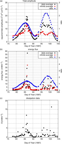
Also shown in Fig. 9a is the ratio between the daily and infinite temporal averages. Note that, for the purpose of visualisation, this ratio is multiplied by 10. It is solely tied to the spring-neap tidal effect, and is not affected by the bathymetry. It also closely follows the spring-neap variation of the 24-hours running average of U ²+V ² (not shown) obtained at the geographical point (18.5°W, 21°S), roughly located in the centre of the BBTRE2 region. The ratio between the daily and infinite temporal averaging can therefore be regarded as the spring-neap tidal cycle associated with the BBTRE2 survey.

Figure 9b shows the temporal average of the calculated energy flux C _Δt over the last 24 hours, the infinite temporal average of the calculated energy flux C _∞, as well as the ratio between the two, at the same stations as in Figure 9a. The ratio between the daily and infinite-time averages is nearly identical to the corresponding ratio in Figure 9a. Thus, this ratio C _Δt /C _∞ (the blue dots in Fig. 9b) only depends on the phase of the spring-neap tidal cycle, and is independent of the bathymetry. Conversely, C _∞ (the red dots) depends only on the bathymetry. The final estimate of the energy flux (the black dots in Fig. 9b) is the product of these two variables.

Figure 9c shows the observed dissipation rates vertically integrated from the near-bottom up to 2500 m above the bottom, D ₂₅₀₀, at the same stations as in Fig. 9a and b. All the values in Fig. 9b (C _Δt /C _∞, C _∞, and C _Δt ) are well correlated with the dissipation rates. However, the interpretation of the results is made difficult by the high correlation between C _Δt /C _∞ (the blue dots) and C _∞ (the red dots), which is evident from Fig. 9b, although these two values are actually independent, since C _Δt /C _∞ depends only on the timing, and C _∞ depends only on the bathymetry.

Appendix C discusses how the correlation between the sum of two variables, here log(C _Δt /C _∞) and log(C _∞), and a third variable, here log(D), depends on the separate correlation between the different pairs of variables. It is shown that if log(C _Δt /C _∞) and log(C _∞) are perfectly correlated, the correlation r(log(C _Δt /C _∞)+log(C _∞), log(D))=r(log(C _Δt ), log(D)) is a weighted linear average of r(log(C _Δt /C _∞), log(D)) and r(log(C _∞), log(D)). Thus, even though each of the variables is positively correlated with the dissipation data, taking both variables into account does not improve the correlation. This is natural, since two perfectly correlated data sets contain the same information. In such a case, it is impossible to separate the contributions from the two variables to the fit with the data. If, on the other hand, log(C _Δt /C _∞) and log(C _∞) are uncorrelated, then r(log(C _Δt ), log(D)) is larger than the linearly weighted average of r(log(C _Δt /C _∞), log(D)) and r(log(C _∞), log(D)) up to a factor . Thus, the correlation with the dissipation data is improved by taking both variables into account.

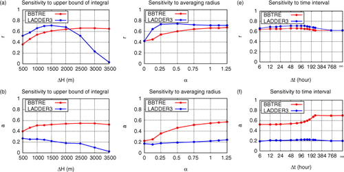
In our case, the correlation is only slightly increased from 0.64 to 0.66 when C _Δt is used instead of C _∞, as seen in Fig. 10e. Thus, the spring-neap tidal cycle is not significantly reflected in the dissipation data. A plausible interpretation of this is the unfortunate accidental correlation between log(C _Δt /C _∞) and log(C _∞) seen in Fig. 9b.

Fig. 10 (a) The correlation coefficient, r, between the energy flux log₁₀(C _Δt ) and the depth-integrated energy dissipation rate log₁₀(D _ΔH ) for various integration heights above the bottom ΔH. The weighted average from all the grid points located within the radius γM ₂ is used to obtain the instantaneous vertical energy flux C at the observational points, which is then averaged over the last 72 hours of the time series, Δt=72 hours. (b) As in (a), but for the slope a of the fit line. (c) Correlation coefficient, r, for different averaging radii, αγM ₂. Here, ΔH=2500 m for BBTRE and 1500 m for LADDER3, and Δt=72 hours. (d) As in (c), but for the slope a of the fit line. (e) The correlation coefficient for various time intervals Δt. ∞ on the horizontal axis corresponds to the long-term average of C, or C _∞. Here, ΔH=2500 m for BBTRE and 1500 m for LADDER3, and α = 1. (f) As in (e), but for the slope a of the fit line.

Appendix C also discusses how the slope of the best-fit line for a sum of two variables against a third variable depends on the separate slopes. The conclusion is that if log(C _Δt /C _∞) and log(C _∞) are uncorrelated, then the slope a(log(C _Δt ), log(D)) is a linearly weighted average of a(log(C _Δt /C _∞), log(D)) and a(log(C _∞), log(D)). If, on the other hand, log(C _Δt /C _∞) and log(C _∞) are positively correlated, then the slope a(log(C _Δt ), log(D)) is smaller than the weighted average of the two other slopes. This explains the result that the slope for BBTRE is significantly larger when using the infinite-time average C _∞ than when averaging over one or a few days (Fig. 10f). Clearly, this can be explained by the unfortunate correlation between log(C _Δt /C _∞) and log(C _∞), and it should not be taken as a sign that C _∞ gives a better agreement with the dissipation data than C _Δt .

When plotting log(D) as a function of log(C _∞), the dependence on the spring-neap tidal cycle is suppressed, and instead manifests itself as a stronger dependence on topography, since the topography is highly correlated with the spring-neap tidal cycle. Hopefully, such an unfortunate correlation can be avoided when planning future cruises with microstructure measurements, since the only way of uniquely associating the observed dissipation with internal tides is to correlate it with the spring-neap tidal cycle. Therefore, calculations of the energy flux could be helpful when planning such cruises.

4. Sensitivity to averaging parameters

In the Section 3, we presented the results which were based on the optimal values of ΔH, α, and Δt. In this section, we explain how these optimal values were obtained by conducting a sensitivity test of the correlation coefficient to ΔH, α, and Δt.

4.1. Upper bound of integration ΔH

We now examine the correlation coefficient for a wide variety of ΔH used for the vertical integration of the dissipation rates. While doing this, we keep the temporal averaging interval fixed at Δt=72 hours and the spatial averaging parameter fixed at α=1.

Figure 10a shows the correlation coefficient. For the BBTRE case, the correlation is significant for most heights, given that the corresponding p values do not statistically differ from zero. The best correlation coefficient is r=0.66 with the steepest fitted-line slope a=0.55 (Fig. 10b). For LADDER3, the correlation is also significant for most values of heights above the bottom, with the best value, r=0.71, attained for ΔH=1500 m, although the slope is small in this case (Fig. 10b).

The values of ΔH at which the highest correlation is obtained, namely, ΔH=2500 m for BBTRE and ΔH=1500 m for LADDER3, are chosen the optimal values for the upper bound of integration.

4.2. Averaging radius α

The sensitivity of the correlation coefficient to the averaging radius is assessed by varying the parameter α in the range 0.125–1.25. This is also supplemented with the case in which a bilinear interpolation of the energy flux to the observational site from the four closest grid points is performed. This case is referred to as α=0.

Figure 10c and d show the variations of r and a as a function of α, respectively. For BBTRE, the correlation coefficient seems to saturate for α values greater than 1. For LADDER3, the best correlation is found for α=0.5. However, the steepest fitted-line slope is found in both cases for the largest radius α=1.25. These results indicate that the energy dissipation at a certain station depends not only on the local energy flux, but also on the integrated energy flux within a radius of the order of the wavelength of the first internal wave mode. This is quite natural, since wave generation is a non-local process.

For a radius larger than γM ₂(α>1), the computational expense increases rapidly, in particular, when a very long time series, for example, 2 weeks, is required for the optimisation process. On the other hand, there is only a slight change in both the correlation and fitted-line slope when the radius larger than γM ₂ is adopted. Thus, α=1 is a good trade-off, and is regarded as the optimal value for the averaging radius.

4.3. Time averaging interval Δt

The sensitivity of the correlation coefficient to the time interval Δt used for the temporal average of C, ranging from 6 to 714 hours (29.75 d) before the observation, is also examined (see Fig. 10e and f). The infinite temporal averaging is given by the value of the time-independent conversion rate C _∞ (see Appendix B).

For BBTRE, the best correlation is obtained for Δt=96 hours (Fig. 10e), although it varies only weakly with Δt. The fitted-line slope a changes from 0.52 to 0.70 (Fig. 10f). Somewhat counterintuitively, this does not imply that C _∞ agrees better than C _Δt with the dissipation data. Instead, this is caused by the unfortunate correlation between the spring-neap tidal cycle and the roughness of the bottom topography in the observational data. This is discussed in more detail in Section 3.4 and in Appendix C.

For LADDER3, the best correlation in conjunction with the steepest fitted line is obtained for a time interval of 120 hours, and similar values are obtained with the interval 72 hours. The fitted-line slope does not change significantly. The value of Δt=72 hours is used as the optimal value for the time averaging interval.

5. Summary and conclusions

A comparison has been made between the calculated internal-tide vertical energy flux and the depth-integrated energy dissipation rate obtained from different microstructure datasets. For the most abundant data, which came from the BBTRE conducted in a large region of rough bottom topography near the Mid-Atlantic Ridge, a good correlation between the calculated energy flux and the observed dissipation rate was found. The best correlation was obtained when averaging the energy flux over the last 3 d prior to the observations, and over an area around the observational site with a radius of the same order as the horizontal wavelength of the first internal wave mode. This indicates that most of the observed dissipation is caused by waves generated in this area. For the BBTRE data, the observed local energy dissipation rate in the lowest 2500 m was around one third of the calculated energy flux for BBTRE data (Fig. 4a). A similar ratio of the observed energy dissipation rate to the calculated energy flux was found for the GRAVILUCK survey, located at the Mid-Atlantic Ridge in the North Atlantic. For LADDER3 conducted over the EPR, on the other hand, the observed dissipation rate in the lowest 1500 m was almost two orders of magnitude smaller than the calculated vertical energy flux (Fig. 4b), and for the IZU data, collected in the west Pacific, it was more than one order of magnitude smaller (Fig. 4d). A summary of the results of the comparison between the energy flux and the dissipation rate for the BBTRE, LADDER3, GRAVILUCK, and IZU datasets is given in Table 1.

Why is the ratio of the energy dissipation to the energy flux much smaller in the Pacific surveys? Both the LADDER3 and IZU were conducted near isolated ridges or seamounts. This may imply that almost all the wave energy escapes from the region before being subject to dissipation. In contrast, our results indicate that dissipation in Brazil Basin is fairly local. Non-linear wave–wave interaction is a key process in cascading the energy from internal waves to turbulent dissipation. The wave energy therefore dissipates more rapidly in regions where the general level of the wave energy is higher, such as at the Mid-Atlantic Ridge, with extended sharp topography. Scattering on the bottom topography also contributes to this cascade, which again makes the dissipation more local in the Brazil Basin.

The fact that the local dissipation efficiency q [see eq. (9)] varies significantly from one region to another conflicts with the standard practice of using a constant q, generally around 0.3, in the parameterisation of tidally induced mixing in current Ocean General Circulation Models (OGCMs). Many more microstructure observations, in more diverse regions, will be needed to obtain a better understanding of the relationship between tidal generation and dissipation. This would allow us to improve parameterisations of the vertical mixing and enable us to make more realistic simulations of the global ocean circulation.

We also investigated the issue of the fortnightly modulation discernible in the vertically integrated dissipation data from BBTRE2 (Fig. 9). We found a striking co-variability both between the vertically integrated energy dissipation rate D and the spring-neap tidal cycle, and between D and the time-independent energy flux C _∞. Hence, both the spring-neap cycle and the bathymetric roughness contribute to the variability of D. Unfortunately, however, the accidental co-variability between the spring-neap tidal cycle and the time-independent energy flux makes it difficult to separate the role of the tidal amplitude from that of the underlying bathymetric roughness. This co-variability is an unfortunate consequence of the timing of the cruise and should be avoided in future cruise plans. A simple way of doing this is to revisit the same stations at different phases of the spring-neap tidal cycle.

The accuracy of the calculated vertical energy flux using linear wave theory is limited by several factors. In particular, the result is sensitive to small-scale details of the bathymetry which are still poorly known in most regions of the ocean. Also, the calculations are invalid when the bathymetric slope is supercritical, although a simple correction for supercritical slopes allows to estimate the energy flux in these regions. We have assessed the importance of both these factors (Figs. (5–8)), although a full correction is impossible with the available data. Finally, the calculations are based on the WKB approximation in the vertical direction, so that the vertical energy flux is proportional to the bottom buoyancy frequency N _B , and this dependence on N _B can yield erroneous results for the internal-tide generation by the broad-scale topographic features (Zarroug et al., 2010). To fully account for the detailed structure of the vertical profile of the buoyancy frequency, it is necessary to employ modal decomposition technique, as discussed by Llewellyn Smith and Young (2002).

Finally, we note that the energy pathway from generation to dissipation caused by breaking of internal tides contains a host of processes, for instance, direct shear instability, wave–wave interaction, wave scattering and near-critical reflection, geometric instability and convective instability. A general review is given by St. Laurent and Garrett (2002). Of particular importance are scattering on bottom topography and wave–wave interaction, such as parametric subharmonic instability (PSI). For the M ₂ tidal constituent, PSI is an effective mechanism equatorward of the latitude 28.8° (Hibiya et al., 1998, 2002 2006, 2007; Hibiya and Nagasawa, 2004; MacKinnon and Winters, 2005; Nikurashin and Legg, 2011), which is where the BBTRE, LADDER3, and IZU measurements were conducted. A consideration of these processes is necessary for a full explanation of the widely different values of the local dissipation efficiency q found in different regions, as well as for a prediction of how the dissipation is distributed vertically.

Acknowledgements

We thank Dr. Kurt Polzin for providing the BBTRE data. We also thank Gurvan Madec and an anonymous reviewer for providing us with the fruitful comments, leading to the significant improvement of the manuscript. The Swedish National Infrastructure for Computing (SNIC) is gratefully acknowledged for providing computer time.

7. Appendix

Appendix A: Time-dependent vertical energy flux

Here we derive the expression for the time-dependent vertical energy flux at the bottom (z=0) when the temporal modulation of the tidal amplitude resulting from the superposition of different tidal constituents is taken into account. This is obtained as the product of pressure and velocity perturbations, namely,A1

The pressure and velocity perturbations vary sinusoidally in time with a tidal frequency ω. Thus, for example, p is given by:

where denotes the complex amplitude of p.

Using a linearised hydrostatic Boussinesq model for the equations of motion subject to a radiation condition at the upper boundary z→+∞, Turnewitsch et al. (2008) derived an expression for as followsA2

where ρ ₀ is the reference water density, f is the Coriolis parameter, and , are the complex amplitudes of the background barotropic velocities. Here the buoyancy frequency N is assumed to be constant and is defined as , with the horizontal mean density. Finally, J represents a two-dimensional convolution between h and ,A3

with .

In the real ocean with finite depth, the largest internal wave scale is given by the horizontal wavelength of the first internal wave mode. Llewellyn Smith and Young (2002) showed that wave generation from topographic features larger than this scale is strongly suppressed. We can thus extend our approach to the case of an ocean with finite depth in an approximate way by replacing 1/2πr by a filtered Green function g _γ(r) (Nycander, 2005),

where

Here I ₀ is the modified Bessel function of the first kind and γ(ω) is the cutoff length obtained by the same expression as in eq. (1), but using the tidal frequency ω. The expression for J thus becomes,A4

Under the WKB approximation, we can further replace the value of N in eq. (A2) by the buoyancy frequency near the ocean floor N _B . The numerical scheme for the computation of the convolution integral J is discussed in detail by Green and Nycander (2013).

Using eq. (A2) and the linearised bottom-boundary condition, w and p at the bottom are given by:A5 A6

where the eight major tidal components have been retained.

Appendix B: Time-independent vertical energy flux

We have seen in Appendix A that the total instantaneous vertical energy flux C is not a linear superposition of the constituent fluxes, because the energy flux is a quadratic quantity, containing terms such as . However, the long-term average of these cross terms vanishes and the time-averaged energy flux can thus be seen as a superposition of time-averaged fluxes of various constituents.

Following Nycander (2005), the expression for the time-independent (or time-average) energy flux P _c for the specified component is given by,

where U₊ and U₋ are velocities along the major and minor tidal-ellipse axes, respectively, x and y axes are chosen to lie along the major and minor axes of the tidal ellipse, and g _γ is given in Appendix A. To determine the total energy flux, we first transform the above equation for P _c to the longitude–latitude coordinate system, and then add the values P _c for eight tidal constituents, namely,

Correction for supercritical slopes

Linear wave theory used here to determine the vertical energy flux is not valid if the bottom slope is supercritical, that is, if the steepness parameter is greater than unity such thatB1

While the energy flux is proportional to in the subcritical regime, it probably saturates when the bottom slope is supercritical (Nycander, 2006). Melet et al. (2013) suggested a simple correction that takes into account supercritical slopes. While they applied this correction to estimate M ₂ energy fluxes only, we applied it to estimate the energy flux by eight major tidal constituents, such that

where

Appendix C: On the fitted-line slope and the correlation coefficient for a sum of two variables

The correlation between the logarithmic values of the vertically integrated dissipation D and the energy flux C is lower when using log(C _∞) than log(C _Δt ) in the BBTRE case, while the fitted-line slope is larger. Here we investigate this by noting that log(C _Δt )=log(C _Δt /C _∞)+log(C _∞). Consequently, we need to understand how the fitted-line slope and the correlation between the sum of two variables, say X=log(C _Δt /C _∞) and Y=log(C _∞), with a third variable, say Z=log(D), depends on the separate correlation between the different pairs of variables, namely (X, Z) and (Y, Z). From the eq. (4), it follows thatB2

Using the identities cov(X+Y, Z)=cov(X, Z)+cov(Y, Z), and var(X+Y)=var(X)+var(Y)+2cov(X, Y), we haveB3

Expressing the covariances in terms of correlations, by using eq. (4), we obtainB4

We can regard this as a weighted average between r(X, Z) and r(Y, Z). The result depends on the correlation r(X, Y) of the ‘input data’. For instance, when there is a perfect correlation between the data sets r(X, Y)=1, eq. (B4) becomes:B5

This is a simple linearly weighted average, with the spread and of the individual data sets as weights.

In the case of the uncorrelated input data sets r(X, Y)=0, eq. (B4) becomes:B6

We see that r(X+Y, Z) is up to a factor larger than the linear average if X and Y are uncorrelated. We conclude that including both input variables X and Y in the statistical model improves the correlation if they are uncorrelated, but not if they are perfectly correlated.

We now consider the slope a of the combined dataset X+Y. Using eq. (6) and following the similar procedure as above, we obtain:B7

For the case of r(X, Y)=0, eq. (B7) yieldsB8

This is a simple linearly weighted average, with var(X) and var(Y) as weights. If, on the other hand, r(X, Y) is positive, the slope a(X+Y, Z) is up to a factor 2 smaller than the linear average given by eq. (B8). Clearly, this does not mean that it is better to include only of the input variables in the statistical models than including both of them. This explains why the slope of log(D) versus log(C _Δt ) is much smaller than that of log(D) versus log(C _∞) for BBTRE, as seen in Fig. 10f.

As a final remark, we note that in the regression of Z on X to find a best-fit line, it is assumed that there is no uncertainty associated with X. However, if X is subject to uncertainties, the slope of best-fit line is biased low. This effect is known as attenuation bias. A simple way to understand it is to note that if X and Z are uncorrelated, the slope of the best-fit line zero both when Z is plotted as a function of X and when X is plotted as a function of Z, as immediately follows from eq. (4). A review accompanied by suggested correction methods is given by Gillard and Iles (2009). They mentioned that the fit-line slope a when both variables Z and X are subject to uncertainties can be an intermediate value between a ₁ and 1/a ₂, resulting from the following regressions:

As an example, for the case of BBTRE when Z=log(D) and X=log(C _Δt ) with Δt=72 hours, a ₁ and a ₂ are found to be 0.5458 and 0.7842, respectively. Hence, 0.5458<a<1.2752. When X=log(C _∞) is used, 0.6982<a<1.8281. It further implies that the uncertainty in the slope of fit line is large. Moreover, a slope of unity, that is, proportionality between D and C, is well within the uncertainty limits.

References

- Alford M. H. , MacKinnon J. A. , Nash J. D. , Simmons H. , Pickering A. , co-authors . Energy flux and dissipation in Luzon Strait: two tales of two ridges. J. Phys. Oceanogr. 2011; 41: 2211–2222.
- Bell T. H . Lee waves in stratified flows with simple harmonic time dependence. J. Fluid Mech. 1975a; 67: 705–722.
- Bell T. H . Topographically generated internal waves in the open ocean. J. Geophys. Res. 1975b; 80: 320–327.
- Buijsman M. C. , Legg S. , Klymak J. M . Double-ridge internal tide interference and its effect on dissipation in Luzon Strait. J. Phys. Oceanogr. 2012; 42: 1337–1356.
- Carter G. S. , Merrifield M. A. , Becker J. M. , Katsumata K. , Gregg M. C. , co-authors . Energetics of M2 Barotropic-to-Baroclinic tidal conversion at the Hawaiian Islands. J. Phys. Oceanogr. 2008; 38: 2205–2223.
- Egbert G. D. , Erofeeva S . Efficient inverse modeling of barotropic ocean tides. J. Atmos. Oceanic Technol. 2002; 19: 183–204.
- Egbert G. D. , Ray R. D . Estimate of M2 tidal dissipation from TOPEX/Poseidon altimeter data. J. Geophys. Res. 2001; 106(C10): 22475–22510.
- Egbert G. D. , Ray R. D . Significant dissipation of tidal energy in the deep ocean inferred from satellite altimeter data. Nature. 2002; 405: 775–778.
- Garrett C. , Kunze E . Internal tide generation in the deep ocean. Ann. Rev. Fluid Mech. 2007; 39: 57–87.
- Gillard J. , Iles T . Methods of fitting straight lines where both variables are subject to measurement error. Curr. Clin. Pharmacol. 2009; 4(3): 164–171.
- Gouretski V. , Koltermann K . WOCE global hydrographic climatology. Berichtedes Bundesamtes für Seeschifffahrt undHydrographi. 2004. 35/2004. 55 pp.
- Green M. , Nycander J . A comparison of tidal conversion parameterizations for tidal models. J. Phys. Oceanogr. 2013; 43: 104–119.
- Hibiya T. , Furuichi N. , Robertson R . Assessment of fine-scale parameterizations of turbulent dissipation rates near mixing hotspots in the deep ocean. Geophys. Res. Lett. 2012; 39: 1–6.
- Hibiya T. , Nagasawa M . Latitudinal dependence of diapycnal diffusivity in the thermocline estimated using a finescale parameterization. Geophys. Res. Lett. 2004; 31: 1–4.
- Hibiya T. , Nagasawa M. , Niwa Y . Nonlinear energy transfer within the oceanic internal wave spectrum at mid and high latitudes. Geophys. Res. Lett. 2002; 107: 28-1–28-8.
- Hibiya T. , Nagasawa M. , Niwa Y . Global mapping of diapycnal diffusivity in the deep ocean based on the results of expendable current profiler (XCP) surveys. Geophys. Res. Lett. 2006; 33: 03611.
- Hibiya T. , Nagasawa M. , NIwa Y . Latitudinal dependence of diapycnal diffusivity in the thermocline observed using a microstructure profiler. Geophys. Res. Lett. 2007; 34: 24602.
- Hibiya T. , Niwa Y. , Fujiwara K . Numerical experiments of nonlinear energy transfer within the oceanic internal wave spectrum. Geophys. Res. Lett. 1998; 103: 18715–18722.
- Klymak J. M. , Legg S. , Pinkel R . A simple parametrization of turbulent tidal mixing near supercritical topography. J. Phys. Oceanogr. 2010; 40: 2059–2074.
- Klymak J. M. , Moum J. N. , Nash J. D. , Kunze E. , Girton J. B. , co-authors . An estimate of tidal energy lost to turbulence at the Hawaiian ridge. J. Phys. Oceanogr. 2006; 36: 1148–1164.
- Ledwell J. R. , Montgomery E. T. , Polzin K. L. , Laurent L. C. S. , Schmitt R. W. , co-authors . Evidence for enhanced mixing over rough topography. Nature. 2000; 403: 179–182.
- Liang X. , Thurnherr A. M . Eddy-modulated internal waves and mixing on a midocean ridge. J. Phys. Oceanogr. 2012; 42(7): 1242–1248.
- Llewellyn Smith S. G. , Young W. R . Conversion of the barotropic tide. J. Phys. Oceanogr. 2002; 32: 1554–1566.
- MacKinnon J. A. , Winters K. B . Subtropical catastrophe: significant loss of low-mode tidal energy at 28.9 degrees. Geophys. Res. Lett. 2005; 32: 15605.
- Melet A. , Nikurashin M. , Muller C. , Falahat S. , Nycander J. , co-authors . Internal tide generation by Abyssal Hills using analytical theory. J. Geophys. Res. 2013; 118: 6303–6318.
- Montgomery E. T . Use of the High Resolution Profiler (HRP) in the Brazil Basin Tracer Release Experiment. 1998; 38. Technical Report WHOI-98-08, Woods Hole Oceanographic Institution, Woods Hole, MA.
- Muller C. J. , Bühler O . Saturation of the internal tides and induced mixing in the abyssal ocean. J. Phys. Oceanogr. 2009; 39: 2077–2096.
- Munk W. , Wunsch C . Abyssal recipes II: energetics of tidal and wind mixing. Deep Sea Res. I. 1998; 45: 1977–2010.
- Nikurashin M. , Ferrari R . Radiation and dissipation of internal waves generated by geostrophic flows impinging on small-scale topography: theory. J. Phys. Oceanogr. 2010a; 40: 1055–1074.
- Nikurashin M. , Ferrari R . Radiation and dissipation of internal waves generated by geostrophic flows impinging on small-scale topography: application to the Southern Ocean. J. Phys. Oceanogr. 2010b; 40: 2025–2042.
- Nikurashin M. , Legg S . A mechanism for local dissipation of internal tides generated at rough topography. J. Phys. Oceanogr. 2011; 41: 378–395.
- Niwa Y. , Hibiya T . Three-dimensional numerical simulation of M 2 internal tides in the East China Sea. J. Geophys. Res. 2004; 109: 04027.
- Niwa Y. , Hibiya T . Estimation of baroclinic tide energy available for deep ocean mixing based on three-dimensional global numerical simulations. J. Oceanogr. 2011; 67: 493–502.
- Nycander J . Generation of internal waves in the deep ocean by tides. J. Geophys. Res. 2005; 110: 10028.
- Nycander J . Tidal generation of internal waves from a periodic array of steep ridges. J. Fluid Mech. 2006; 567: 415–432.
- Polzin K. L . Idealized solutions for the energy balance of the finescale internal wave field. J. Phys. Oceanogr. 2004; 34: 231–246.
- Polzin K. L . An abyssal recipe. Ocean Modell. 2009; 30: 298–309.
- Polzin K. L. , Toole J. M. , Ledwell J. R. , Schmitt R. W . Spatial variability of turbulent mixing in the abyssal ocean. Science. 1997; 276: 93–96.
- Samelson R. M . Large-scale circulation with locally enhanced vertical mixing. J. Phys. Oceanogr. 1998; 28: 721–726.
- St Laurent L. C. , Garrett C. J. R . The role of internal tides in mixing the deep ocean. J. Phys. Oceanogr. 2002; 32: 2882–2899.
- St Laurent L. C. , Simmons H. L. , Jayne S. R . Estimating tidally driven mixing in the deep ocean. Geophys. Res. Lett. 2002; 29: 2106.
- St Laurent L. C. , Thurnherr A. M . Intense mixing of lower thermocline water on the crest of the mid-Atlantic ridge. Nature. 2007; 448: 680–683.
- St Laurent L. C. , Toole J. M. , Schmitt R. W . Buoyancy forcing by turbulence above rough topography in the abyssal Brazil Basin. J. Phys. Oceanogr. 2001; 31: 3476–3495.
- Thurnherr A. M. , St Laurent L. C . Turbulence and diapycnal mixing over the east pacific rise crest near 10°N. Geophys. Res. Lett. 2011; 38: 15613.
- Thurnherr A. M. , St Laurent L. C. , Speer K. G. , Toole J. M. , Ledwell J. R . Mixing associated with sills in a canyon on the mid ocean ridge flank. J. Phys. Oceanogr. 2005; 35: 1370–1381.
- Toole J. M . Temporal characteristics of abyssal finescale motions above rough bathymetry. J. Phys. Oceanogr. 2007; 37: 409–427.
- Toole J. M. , Ledwell J. R. , Polzin K. L. , Schmitt R. W. , Montgomery E. T. , co-authors . The Brazil Basin tracer release experiment. WOCE Int. Newslett. 1997; 28: 25–28.
- Turnewitsch R. , Reyss J. L. , Nycander J. , Waniek J. J. , Lampitt R. S . Internal tides and sediment dynamics in the deep sea-evidence from radioactive 234Th/238U disequilibria. Deep Sea Res. I. 2008; 55: 1727–1747.
- Van Haren H . Asymmetric vertical internal wave propagation. Geophys. Res. Lett. 2006; 33(6): 06618.
- Wunsch C. , Ferrari R . Vertical mixing, energy, and the general circulation of the oceans. Annu. Rev. Fluid Mech. 2004; 36: 281–314.
- Zarroug M. , Nycander J. , Döös K . Energetics of tidally generated internal waves for nonuniform stratification. Tellus A. 2010; 62: 71–79.
- Zhang J. , Schmitt R. W. , Huang R. X . The relative influence of diapycnal mixing and hydrologic forcing on the stability of the thermohaline circulation. J. Phys. Oceanogr. 1999; 29: 1096–1108.
- Zilberman N. V. , Becker J. M. , Merrifield M. A. , Carter G. C . Model estimate of M2 internal tide generated over mid-Atlantic ridge topography. J. Phys. Oceanogr. 2009; 39: 2635–2651.