Estimating correlated observation error statistics using an ensemble transform Kalman filter

Abstract

For certain observing types, such as those that are remotely sensed, the observation errors are correlated and these correlations are state- and time-dependent. In this work, we develop a method for diagnosing and incorporating spatially correlated and time-dependent observation error in an ensemble data assimilation system. The method combines an ensemble transform Kalman filter with a method that uses statistical averages of background and analysis innovations to provide an estimate of the observation error covariance matrix. To evaluate the performance of the method, we perform identical twin experiments using the Lorenz '96 and Kuramoto-Sivashinsky models. Using our approach, a good approximation to the true observation error covariance can be recovered in cases where the initial estimate of the error covariance is incorrect. Spatial observation error covariances where the length scale of the true covariance changes slowly in time can also be captured. We find that using the estimated correlated observation error in the assimilation improves the analysis.

• data assimilation
• correlated observation errors
• ensemble transform Kalman filter

1. Introduction

Data assimilation techniques combine observations with a model prediction of the state, known as the background, to provide a best estimate of the state, known as the analysis. The errors associated with the observations can be attributed to four main sources:

1. Instrument error.

2. Error introduced in the observation operator – these include modelling errors, such as the misrepresentation of gaseous constituents in radiative transfer models, and errors due to the approximation of a continuous function as a discrete function.

3. Errors of representativity – these are errors that arise where the observations can resolve spatial scales that the model cannot.

4. Pre-processing errors – errors introduced by pre-processing of the data such as cloud clearance for radiances.

For a data assimilation scheme to produce an optimal estimate of the state, the error covariances associated with the observations and background must be well understood and correctly specified (Houtekamer and Mitchell, 2005). In practice, many assumptions are violated and the analysis provided by the assimilation may be far from optimal. Therefore to obtain an accurate analysis, it is important to have good estimates of the observation and background error covariance matrices to be used in the assimilation.

In previous work, much attention has been given to the estimation of the background error covariance matrix and as a result static background error covariance matrices are now often replaced with flow-dependent matrices that reflect the ‘errors of the day’ (Bannister, 2008). Until recently, less emphasis has been given to understanding the nature of the observation error covariance matrix and the matrix is often assumed diagonal. The unknown errors, such as the representativity error, and any other possible unaccounted for correlations, are represented by inflating the error variance (Whitaker et al., 2008; Hilton et al., 2009), or by using techniques such as observation thinning (Buehner, 2010) or ‘superobbing’ (Daley, 1991).

One difficulty in quantifying observation error correlations is that they can only be estimated in a statistical sense, not calculated directly. The distinction between biased and correlated errors can be a particular issue. For example, Stewart et al. (2013), report that ‘a series of correlated samples will tend to be smoother than a series of independent samples, with adjacent and nearby values more likely to be similar. Hence, in practical situations it would be easy for a sample from a correlated distribution with a zero mean to be interpreted as a biased independent sample (Wilks, 1995)’.

Despite the challenges in estimating correlated errors, recent works, for example, Stewart et al. (2009, 2014), Bormann et al. (2002), Bormann and Bauer (2010), Bormann et al. (2010), using the methods of Hollingsworth and Lönnberg (1986) and Desroziers et al. (2005) have shown that for certain observing instruments the observation error covariance matrix is correlated. When these correlated errors have been accounted for in the assimilation, it has been shown to lead to a more accurate analysis (Healy and White, 2005; Stewart, 2010; Stewart et al., 2013), the inclusion of more observation information content (Stewart et al., 2008) and improvements in the UK Met Office skill score (Weston, 2011; Weston et al., 2014). Indeed, Stewart et al. (2013) and Healy and White (2005) reported that even the use of a crude approximation to the observation error covariance matrix may provide significant benefit.

The importance of accounting for correlated errors in the assimilation has led to the development of new schemes that provide estimates of the observation error covariance matrix. The methods of Li et al. (2009) and Miyoshi et al. (2013) use the diagnostic of Desroziers et al. (2005) (hereafter denoted as the DBCP diagnostic), embedded in a local ensemble transform Kalman filter (ETKF) to derive estimates of an observation error covariance matrix, assumed in their study to be static. With this method, an initial estimate of the observation error covariance matrix is updated incrementally using statistics averaged over each observation type at each assimilation step. This method assumes that all observations of a given type share the same variances and spatial correlation structure. The method is limited by the availability of samples. More significantly, the authors have not shown that it permits true correlations that are spatially varying over time to be estimated. It has been demonstrated, however, that representativity errors are dependent on both time and space (Janjic and Cohn, 2006; Waller et al., 2014).

In this paper, we introduce a method that combines an ensemble filter with the DBCP diagnostic. In this method, the observation error covariance matrix is estimated using statistics averaged over a rolling time window. This removes the assumption that each observation of a given type shares the same variances and correlations and enables a true correlation matrix that is spatially and temporally varying to be estimated and incorporated in the assimilation scheme.

In Section 2, we describe the ensemble filter that can be used to provide a time-varying estimate for correlated observation error. Our experimental design is given in Section 3 and we present our numerical results in Section 4. We show that, as demonstrated in experiments using simple models, it is possible to use the proposed method to provide an estimate of spatial observation error correlations that vary slowly in time. Finally, we conclude in Section 5.

2. Estimating the observation error covariance matrix with the ETKF

Data assimilation techniques combine observations at time t _n with a model prediction of the state, the background , which is often determined by a previous forecast. Here N ^p and N ^m denote the dimensions of the observation and model state vectors, respectively. The observations and background are weighted by their respective error statistics, to provide a best estimate of the state , known as the analysis. This analysis is then evolved forward in time, using the possibly non-linear model , to provide a background at the next assimilation time. Under the perfect model assumption, we have1

We now give a brief overview of the ETKF (Bishop et al., 2001; Livings et al., 2008) that we adapt here and the notation that is used in this study. At time t _n we have an ensemble, a statistical sample of N state estimates for . These ensemble members are stored in a state ensemble matrix , where each column of the matrix is a state estimate for an individual ensemble member,2

It is possible to calculate the ensemble mean,3

and subtracting the ensemble mean from the ensemble members gives the ensemble perturbation matrix4

This allows us to write the ensemble error covariance matrix as5

When the forecast error covariance is derived from climatological data and assumed static, it is often denoted as B and known as the background error covariance matrix.

For the ETKF, the analysis at time t _n is given by,6

where is the analysis ensemble mean and is the forecast ensemble mean. The possibly non-linear observation operator maps the model state space to the observation space. The Kalman gain matrix,7

is a matrix of size N ^m ×N ^p . The matrix is a matrix of size N ^p ×N ^p , where is defined as the matrix containing the mapping of the ensemble perturbations into observation space using the linearised observation operator H _n and the observation error covariance matrix is denoted by . The matrix S _n is invertible if it is full rank. In the ETKF, we usually assume R _n is symmetric and positive definite (i.e. full rank) since is typically of low rank.

Previously, it has been assumed that the observation error covariance matrix R is diagonal. However, with recent work showing that R is correlated and state dependent, it is important to be able to gain accurate estimates of the observation error covariance matrix. Here, we propose a method that combines the DBCP diagnostic with an ETKF (Bishop et al., 2001). This method provides a new technique for estimating time-varying correlated observation error matrices that can be used within the assimilation scheme. We begin by describing the diagnostic proposed in Desroziers et al. (2005).

2.1. The DBCP diagnostic

The DBCP diagnostic described in Desroziers et al. (2005) makes use of the background (forecast) and analysis innovations to provide an estimate of the observation error covariance matrix. The background innovation, , is the difference between the observation y and the mapping of the forecast vector, x ^f , into observation space by the observation operator . The analysis innovations, , are similar to the background innovations, but with the forecast vector replaced by the analysis vector x ^a . Taking the statistical expectation, E, of the outer product of the analysis and background innovations and assuming that the forecast and observation errors are uncorrelated results in8

This is valid if the observation and forecast error covariance matrices used in the gain matrix,9

to calculate the analysis, are the exact observation error covariance matrix and forecast error covariance matrix (Desroziers et al., 2005). However, provided that the correlation length scales in P ^f and R are sufficiently different, it has been shown that a reasonable estimate of R can be obtained even if the R and P ^f used in K are not correctly specified. It has also been shown that the method can be iterated to estimate R (Desroziers et al., 2009; Mènard et al., 2009).

The DBCP diagnostic does not explicitly account for model error. Nevertheless, the diagnostic has been successfully used in complex operational models to estimate correlated observation error covariances, including time invariant non-isotropic inter-channel error correlations (Stewart et al., 2009; Bormann and Bauer, 2010; Bormann et al., 2010; Stewart, 2010; Weston, 2011; Stewart et al., 2014; Weston et al., 2014). However, much of this previous work has considered variational data assimilation methods. As ensemble filters and hybrid methods are becoming more widely used in operational data assimilation (Buehner et al., 2010; Miyoshi et al., 2010; Clayton et al., 2013), we consider the use of the DBCP diagnostic when using an ensemble data assimilation method with flow-dependent forecast error statistics.

2.2. The ETKF with R estimation

We first give a brief overview of the proposed method, the ETKF with R estimation (ETKFR), before discussing it in further detail. The idea is to estimate a possibly non-uniform observation error covariance matrix that varies in time using the ETKF. We use the ETKF to provide samples of the background and analysis innovations to be used in the DBCP diagnostic. After the initial ensemble members, forecast error covariance matrix and observation error covariance matrix are specified, the filter is split into two stages: a spin-up phase where the matrix R remains static and a ‘varying estimate’ stage. The spin-up stage is run for a predetermined number of steps, N ^s , and is an application of the standard ETKF. This stage also allows the structures in the background error covariance matrix to develop. In the second stage, the DBCP diagnostic is calculated using N ^s samples to provide a new estimate of R that is then used within the assimilation. We note that for any assimilation that is running continuously, the spin-up stage need only be run once to determine the initial samples required to estimate R. We now present in detail the method that we have developed. Here the observation operator, H, is chosen to be linear, but the method could be extended to account for a non-linear observation operator (e.g. Evensen, 2003).

Initialisation – Begin with an initial ensemble for at time t=0 that has an associated initial covariance matrix . Also assume an initial estimate of the observation error covariance matrix R ₀; it is possible that this could just consist of the instrument error.

Step 1 – The first step is to use the full non-linear model, , to forecast each ensemble member, .

Step 2 – The ensemble mean and covariance are calculated using (3) and (5).

Step 3 – Using the ensemble mean and the background innovations at time t _n , calculate and store .

Step 4 – The ensemble mean is updated using,10

where K _n is the Kalman gain.

Step 5 – The analysis perturbations are calculated as11

where Γ _n is the symmetric square root of (Livings et al., 2008). Using this method means that no centring technique is required in order to preserve the analysis ensemble mean.

Step 6 – The analysis mean is then used to calculate the analysis innovations, .

Step 7 – If , where N ^s is the specified sample size, update R using12

Then symmetrise the matrix, ). Otherwise keep .

Many of the steps in the proposed method are identical to the ETKF. Step 7, along with the storage of the background and analysis innovations in steps 3 and 6, are the additions to the ETKF that provide the estimate of the observation error covariance matrix. At every assimilation step R is updated using the latest information, with the oldest information being discarded. Although this does not give a completely time-dependent estimate of R it should give a slowly time-varying estimate that should take into account the most recent information relating to the observations. In step 5, rather than calculating the symmetric square root explicitly, it is possible to make use of the fact that . It is then necessary to invert a full R matrix. This may be carried out efficiently using the Cholesky decomposition method. Rather than inverting the matrix at each assimilation step, the decomposition can be updated using rank-1 down and updates with only a small number of operations relative to the dimension of the matrix (Golub and Van Loan, 1996).

The first time a correlated observation error matrix is introduced, it is possible that the assimilation may be affected by the sudden change, although this has not caused any problems in our experiments. In a practical situation, this would only occur once during the spin-up phase and, if necessary, it could be overcome by applying a smoothing to introduce the new matrix over a short period of time.

In general, the optimal number of samples, N ^s , required to estimate R is unknown. Ideally, the number of samples would be larger than the number of entries to be estimated. However, using a larger number of samples means the estimate of the observation error covariance matrix is an average over a large period of time. Hence, the larger the number of samples the less time-dependent the estimate becomes. Therefore, the optimal value of N ^s must be a compromise between the large number of samples required to obtain a good approximation to the matrix and the limited number of samples that allows the time-varying nature of the observation error covariance matrix to be captured.

In practice, the number of samples available will be limited and, therefore, the estimated observation error covariance matrix will not be full rank. In this case, it may be necessary to apply some form of regularisation to the estimated matrix, see Bickel and Levina (2008). This regularisation could, for example, take the form of a covariance localisation to remove spurious long range correlations (Hamill et al., 2001; Bishop and Hodyss, 2009), or the assumption that the correlation function is globally uniform. Weston et al. (2014) used reconditioning techniques to obtain full rank approximations of the matrix and this allowed their estimated matrix to be used successfully in the assimilation.

3. Experimental design

3.1. The models

To demonstrate the potential of the ETKFR approach, we use two different models: the Lorenz '96 model (Lorenz, 1996; Lorenz and Emanuel, 1998) and the Kuramoto-Sivashinsky (KS) equation (Sivashinsky, 1977; Kuramoto, 1978).

3.1.1. The Lorenz '96 model.

The Lorenz '96 model has been widely used to test state estimation problems (Anderson, 2001; Ott et al., 2004; Fertig et al., 2007). The model emulates the behaviour of a meteorological variable around a circle of latitude. The model consists of N ^m variables on a cyclic boundary, that is, , and , which are governed by,13

The first term on the right-hand side simulates advection, whereas the second simulates diffusion, and the third is a constant forcing term. The solution exhibits chaotic behaviour for N ^m ≥12 and F>5 and to ensure that we see chaotic behaviour in our solution we choose N ^m =40 and F=8.

3.1.2. The KS equation.

The KS equation,14

is a non-linear, non-dimensional partial differential equation where u is a function of time, t, and space, x. The equation produces complex behaviour due to the presence of the second- and fourth-order terms. The equation can be solved on both bounded and periodic domains and, when this spatial domain is sufficiently large, the solutions exhibit multi-scale and chaotic behaviour (Eguíluz et al., 1999; Gustafsson and Protas, 2010). This chaotic and multi-scale behaviour makes the KS equation a suitable low dimensional model that represents a complex fluid dynamic system. The KS equation has been used previously for the study of state estimation problems using both ensemble and variational methods (Protas, 2008; Jardak et al., 2010).

3.2. Twin experiments

To analyse the ETKF with R estimation (ETKFR), we perform a series of twin experiments. For our twin experiments, we determine a ‘true’ trajectory by evolving the perfect model equations forward from known initial conditions. From the true trajectory we create observations (see Section 3.2.1). These observations are then used in the assimilation. In the assimilation all the ensemble members are also evolved using the perfect model equations but beginning from perturbed initial conditions. We now describe how we calculate the observations; then we provide details for the experiments using the Lorenz '96 and KS models.

3.2.1. The observations.

To create observations from the true model trajectories we must add errors from a specified distribution. The true observation error covariance matrix, R ^t =R ^D +R ^C , consists of two components, representing the uncorrelated observation error part and the correlated observation error part. The uncorrelated observation covariance matrices are defined as , where is the corresponding error variance and the correlated observation covariance matrices are defined as , where is the corresponding error variance and C is a correlation matrix. We use direct observations with added uncorrelated observation error, which are calculated by adding pseudo-random samples from to the values of the truth. We then add correlated error to our observations. Since we are testing the feasibility of the proposed method, here we consider an isotropic and homogeneous observation error covariance. As the correlation function we use the SOAR function,15

where ρ is the correlation between two points i and j on a circle and θ _i,j is the angle between them (Thiebaux, 1976). The constants L and b determine the length scale of the correlation function and the correlation function is valid on the domain of length 2aπ. We choose the SOAR function to approximate our correlated error because, at large correlation length scales, the SOAR resembles the observation error covariance structure found in Bormann et al. (2002). The SOAR function is used to determine the circulant covariance matrix C. Having a specified observation error covariance matrix allows us to determine how well the method is working as the estimated matrix can be compared to the truth.

3.2.2. Regularising the estimated error covariance matrix.

In our experiments, we make the regularising assumption that the observation error covariance structure is isotropic and homogeneous. Hence, the observation error covariance matrices we use in the assimilation have a circulant structure, which is determined by a single vector, c. This vector occupies the first row of the matrix, the remaining rows being determined by cyclic permutations of the vector c.

To regularise the estimated error covariance matrix R ^est obtained from the ETKFR, we find a vector from which we construct a circulant error covariance matrix R to use in the next assimilation step. To calculate the vector c ^e we first permute the rows of R ^est so that for each row the variance lies in the same column. The averages of these columns are then taken to produce the elements of the vector c ^e that defines circulant matrix R. The estimated vector c ^e can also be compared to the corresponding vector c ^t defining the true circulant error covariance matrix in order to evaluate the performance of the DBCP diagnostic (see Section 4.1).

3.2.3. The Lorenz '96 model.

In this study, we solve the system of equations using MATLAB's (version R2008b) ode45 solver, which is based on an explicit Runge-Kutta formula (Dormand and Prince, 1980); this uses a relative error tolerance of 10⁻³ and an absolute error tolerance of 10⁻⁶. To generate the true solution the Lorenz equations are started from initial conditions where X_j =8, j=1 … 40 with a small perturbation of 0.001 added to variable X ₂₀. The numerical model provides output at intervals of Δt=0.01 until a final time of T=50. To generate the initial ensemble background states, N=500 pseudo-random samples from the distribution , where is the forecast error variance, are added to the true initial condition. A large number of ensemble members is used to minimise the risk of ensemble collapse and to help obtain an accurate forecast error covariance matrix. For the purposes of this initial study, we wish to avoid using the techniques of covariance inflation and localisation so as not to contaminate the estimate of R. We take 20 equally spaced direct observations, calculated as described in Section 3.2.1, at each assimilation step. Constants for eq. (15) are chosen to be L=6 and b=3.6 (unless otherwise stated). We then consider time-dependent R where b varies linearly with time according to b(t) =αt+β. The frequency varies between experiments, with the chosen frequencies being observations available every 5 and 30 time steps, that is, every 0.05 and 0.3 time units, respectively.

3.2.4. The KS equation.

In this study, the KS equation is solved using an exponential time differentiating Runge-Kutta 4 (ETDRK4) numerical scheme. Details of this scheme, along with code to solve the KS equation are given in Cox and Matthews (2000) and Kassam and Trefethen (2005). The truth is defined by the solution to the KS equation on the periodic domain 0≤x≤32π from initial conditions until time T=10000, using N=256 spatial points and a time step of Δt=0.25. The assimilation model is run at the same spatial and temporal resolution as the truth with Δt=0.25 and N=256.

To determine the initial ensemble background states, pseudo-random samples from the distribution , where is the forecast error variance, are added to the true initial condition. For the KS equation we choose to use N=1000 ensemble members as we are estimating a large number of state variables. From the background N=1000 ensemble members are created by adding pseudo-random samples from the initial forecast error distribution, which is chosen also to be . We take 64 equally spaced direct observations, calculated as described in Section 3.2.1, at each assimilation step. Constants for eq. (15) are chosen to be L=15 and b=3.8 (unless otherwise stated); for some experiments b is chosen to vary linearly in time according to . The frequency varies between experiments, with the chosen frequencies being observations available every 40 and 100 time steps. We next present experimental results of applying ETKFR to these models.

4. Results

We carry out a number of experiments to test the performance and robustness of the ETKFR method.

To demonstrate the potential of the proposed methodology, we perform several ETKF runs with the predefined observation error covariance matrix. In these runs, we use either the true observation error covariance (1L, 4L, 7L, 1K, 4K, 7K) or we approximate the observation error covariance through a diagonal one omitting the cross-correlated terms (2L, 5L, 2K, 5K).

We note that the ETKFR has been tested with different frequencies of observations in both time and space. The results presented here have been selected to demonstrate the different behaviours of the method under certain conditions. The method was also run with fewer ensemble members, down to N ^m =50 for the Lorenz '96 model and N ^m =500 for the KS model, and appears to work well. For ensemble sizes smaller than this, the techniques of localisation and inflation would be required for the ETKF itself not to diverge. Experiments have also been run with different realisations of observation and background error noise and it is found that the qualitative results are unchanged. The ETKFR has also been tested with a range of reduced sample sizes, N ^s , with the minimum number of samples being a tenth of those in the results presented. In these cases we find that the assimilation performs qualitatively similarly to the cases shown. As expected the estimate of the covariance is slightly degraded; however, even with the smallest number of samples, the estimates of the covariance matrix appear qualitatively similar to those presented.

For the DBCP diagnostic to provide good estimates of the observation error covariance function it is assumed that the length scales of the background and observation error covariances are sufficiently different. It is not possible to fix the length scale of the background errors as they are determined through the model evolution. However, unless otherwise stated, in general the length scales of the background error correlations are three to five times smaller than those assumed for the observation errors and hence the DBCP diagnostic should perform well (Desroziers et al., 2009).

4.1. Metrics

To evaluate the performance of the method and how well it estimates the covariances, we provide a number of measures. The first measure we present, E1, gives the time-averaged norm of the difference between the analysis at time t _n and the truth at time t _n ,16

where N ^a is the number of assimilation steps.

To allow a comparison between experiments we also give the percentage of the error, E1, with respect to the time-averaged norm of the true solution,17

Rank histograms (Hamill, 2000) (shown in Waller, 2013) were examined to give information about the ensemble spread. If the ensemble spread is not maintained the analysis and the estimation of the observation error covariance matrix may be affected.

We also present metrics for how well the ETKFR estimates the covariance matrix. As the covariance matrix is isotropic and homogeneous, rather than comparing the estimated matrix R to the true matrix R ^t , we compare the vector , at time t _n (described in Section 3.2.2) with the corresponding vector . We compute C1, the time-averaged norm of the difference between the estimated vector, , at time t _n and the true vector, , at time t _n ,18

where N ^ae is the number of assimilation steps at which the observation error covariance is estimated.

Again we provide a percentage, C2, with respect to the true error covariance to allow a comparison between experiments,19

When experiments are run with different realisations of observation and background error noise it is found that the error metric results are unchanged to two decimal places.

We present the results of our experiments in Table and 2 . In Table 1, we consider how the ETKFR method performs against the standard ETKF. In Table 2, we consider how the ETKFR performs under different conditions. In the tables, we give details of the matrix used as the true observation error covariance matrix R ^t . We also give details of the assimilation method used and the R used in the assimilation. We provide the frequency of the observations and the variances for the initial forecast, uncorrelated and correlated error. We present the metrics E1 and E2, and for the experiments using the ETKFR we also present metrics C1 and C2.

Table 1. Details of experiments executed using the Lorenz '96 (L) and Kuramoto-Sivashinsky (K) models to investigate the assimilation performance of the ETKFR compared to the ETKF

Exp. no.	Assimilation method	Obs Freq. (time steps)	E1	E2	C1	C2
1L	ETKF (R=R ^t)	5	0.68	2.3% (29.53)	–	–
2L	ETKF (R=diag R ^t)	5	0.73	2.5% (29.53)	–	–
3L	ETKFR (R 0=R ^D)	5	0.70	2.4% (29.53)	0.02	9.1% (0.22)
4L	ETKF (R=R ^t)	30	2.31	7.8% (29.46)	–	–
5L	ETKF (R=diag R ^t)	30	2.83	9.6% (29.46)	–	–
6L	ETKFR (R 0=R ^D)	30	2.43	8.3% (29.46)	0.04	18.2% (0.22)
7L	ETKF (R=R ^t)	5	0.66	2.2% (29.53)	–	–
8L	ETKFR (R 0=R ^D)	5	0.67	2.3% (29.53)	0.02	8.7% (0.23)
1K	ETKF (R=R ^t)	40	4.00	19.0% (20.98)	–	–
2K	ETKF (R=diag R ^t)	40	4.41	21.0% (20.98)	–	–
3K	ETKFR (R 0=R ^D)	40	4.12	19.6% (20.98)	0.05	17.2% (0.29)
4K	ETKF (R=R ^t)	100	5.65	26.8% (21.05)	–	–
5K	ETKF (R=diag R ^t)	100	6.00	28.5% (21.05)	–	–
6K	ETKFR (R 0=R ^D)	100	5.95	28.3% (21.05)	0.14	48.2% (0.29)
7K	ETKF (R=R ^t)	40	3.89	18.6% (20.98)	–	–
8K	ETKFR (R 0=R ^D)	40	4.07	19.4% (20.98)	0.09	29.0% (0.31)

The experiments are run with R ^t =R ^C +R ^D and . For experiments 1L to 6L the correlation length scale parameter is b=3.6 and for 1K to 6K is b=3.8. For 7L and 8L α=−3×10⁻⁴ and β=3.6 and for 7K and 8K α=3×10⁻⁴ and β=3.7. Note that for different runs of these experiments, the results are unchanged to two decimal places.

Table 2. Details of experiments executed using the Lorenz '96 (L) and Kuramoto-Sivashinsky (K) models to investigate the robustness of the ETKFR

Exp. no.	True R	, ,	E1	E2	C1	C2
9L	α=0, β=5.0	0.1	0.74	2.5% (29.53)	0.02	9.1% (0.22)
10L	α=3×10^−4, β=3.3	0.1	0.68	2.3% (29.53)	0.02	9.1% (0.22)
11L	α=−1×10^−3, β=3.6	0.1	0.68	2.3% (29.53)	0.03	13.0% (0.23)
12L	α=−3×10^−4, β=3.6	0.01	0.21	0.7% (29.53)	0.00	0.0% (0.02)
13L	α=−3×10^−4, β=3.6	1.0	2.43	8.2% (29.53)	0.26	11.6% (2.25)
14L	α=−3×10^−4, β=3.6	0.1, 1.0, 1.0	2.62	8.9% (29.53)	0.26	11.6% (2.25)
15L	α=−3×10^−4, β=3.6	1.0, 0.1, 0.1	0.68	2.3% (29.53)	0.02	8.7% (0.23)
9K	α=0, β=3.5	0.1	4.97	23.7% (20.98)	0.07	25.0% (0.28)
10K	α=−3×10^−4, β=4.0	0.1	4.03	19.2% (20.98)	0.10	34.5% (0.29)
11K	α=4×10^−4, β=3.7	0.1	4.03	19.2% (20.98)	0.10	31.3% (0.32)
12K	α=3×10^−4, β=3.7	0.01	0.95	4.5% (20.98)	0.00	0.0% (0.03)
13K	α=3×10^−4, β=3.7	1.0	11.27	53.7% (20.98)	0.85	27.6% (3.08)
14K	α=3×10^−4, β=3.7	0.1, 1.0, 1.0	11.25	53.6% (20.98)	0.88	28.6% (3.08)
15K	α=3×10^−4, β=3.7	1.0, 0.1, 0.1	4.18	19.9% (20.98)	0.10	32.3% (0.31)

The initial matrix used in the assimilation is always equal to . Observations are available every five time steps for the Lorenz '96 model and 40 time steps for the KS model. Note that for different runs of these experiments, the results are unchanged to two decimal places.

4.2. Performance of the ETKFR

We first consider how the ETKFR performs in comparison with the standard ETKF. Variances corresponding to the initial forecast , uncorrelated and correlated error are all set to 0.1.

4.2.1. Results with a static R and frequent observations.

We begin by examining the case where the observations are available frequently in time. Observations are available every five time steps for the Lorenz '96 model and 40 time steps for the KS model. We set the true static matrix R ^t to R ^t =R ^D +R ^C , where the uncorrelated error covariance is R ^D =0.1I and the correlated error covariance is R ^C =0.1C , where C is the correlation matrix described in Section 3.2.1 with L and b as described in Sections 3.2.3 and 3.2.4. We use the standard ETKF and use the correct static observation error covariance matrix, R ^t , in the assimilation. The Lorenz '96 and KS models are each run for 1000 assimilation steps and results are presented in Table 1 Experiments 1L and 1K, respectively. As the correct error covariance matrices are used, these experiments provide a reference for the best performance we can expect from the assimilation.

In Experiments 2L and 2K we use the standard ETKF for the assimilation, but assume that R is diagonal, with R ₀=diag(R ^t ). The details for these experiments using the Lorenz and KS models are given in Table 1, Experiments 2L and 2K. We see from the errors E1 and percentages E2 that the assimilation performs slightly worse than in the case where the true observation error covariance matrix is used in the assimilation, with the percentage error increasing from 2.3 to 2.5%. However the assimilation still performs well and the rank histogram (not shown) suggests that the ensemble is well spread.

We now consider what happens where we estimate R within the ETKFR assimilation scheme described in Section 2 with N ^s =100 for the Lorenz model and N ^s =250 for the KS model. These values of N ^s are chosen to provide an adequate number of samples to estimate R while still allowing the time-varying nature of the observation error covariance matrix to be captured. For the estimated covariance matrix to be full rank, and hence used in the assimilation, we find it is necessary to regularise the estimated matrix. We regularise the matrix using the method described in Section 3.2.2. This method of regularisation requires no information about the true correlation structure. However, it does make the assumption that all the observations have the same correlation structure. If this assumption is not expected to hold, such as in operational systems, a different method of regularisation may be required. We verify that the method proposed is able to improve the analysis by including improved estimates of R in the assimilation scheme.

We begin by assuming that the initial observation error covariance matrix consists of only the uncorrelated error R ^D . The details and results for these experiments using the Lorenz and KS models are given in Table 1 Experiments 3L and 3K. We see that the errors, E1, and percentages, E2, are lower than Experiments 2L and 2K and this, together with an improved ensemble spread, shows that overall the assimilation scheme performs better than the case where the observation error covariance matrix is assumed diagonal. When considering how the norm of the difference between the analysis x ^a and the truth x ^t varies over time (not illustrated), we see an overall reduction in the error after the spin-up phase once the correlated observation error matrix is included in the assimilation.

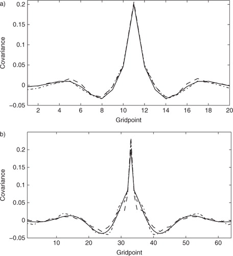
In Fig. 1, we plot the true covariance (solid) as well as the first estimate of the covariance calculated using the first N ^s background and analysis innovations (dashed) and the last estimate of the covariance calculated using the last N ^s background and analysis innovations (dot–dash). We see that the first estimate of the covariance using the DBCP diagnostic gives a good estimate of the true covariance with approximately correct length scales. This suggests that even if a correlated observation error covariance is initially unknown it should be possible to use the DBCP diagnostic to estimate it (Desroziers et al., 2009). This is consistent with results using 4D-Var (Stewart et al., 2009, 2014; Bormann and Bauer, 2010; Bormann et al., 2010) and the ETKF (Miyoshi et al., 2013). We see that the last estimates of the covariance are closer to the true covariance. From the table, we see that on average the covariance for Experiment 3L is more accurate than for the Experiment 3K. This is a result of a proportionally larger number of samples being used to estimate fewer points in the covariance matrix. Overall, the method performs well and this suggests that updating the estimate of R at each assimilation step in the ETKF improves the estimation of a static R. It also suggests that it should be possible to gain a time-dependent estimate of correlated observation error.

Fig. 1 Rows of the true and estimated covariance matrices. (a) Experiment 3L. Rows of the true (solid) and estimated covariance matrices. Covariance calculated using the first 100 background and analysis innovations (dashed). Covariance calculated using the last 100 background and analysis innovations (dot–dashed). (b) Experiment 3K. Rows of the true (solid) and estimated covariance matrices. Covariance calculated using the first 250 background and analysis innovations (dashed). Covariance calculated using the last 250 background and analysis innovations (dot–dashed).

4.2.2. Static R , infrequent observations.

We keep the true matrix R ^t static, as in the previous section, but now consider the case where the observations are less frequently available. Observations are available only every 30 time steps (six times less frequent) for the Lorenz '96 model and 100 time steps (2.5 times less frequent) for the KS model; therefore we have statistics from 166 to 400 assimilation steps. We keep the value of N ^s at 100 for the Lorenz '96 model and 250 for the KS model. We again begin by showing the best performance we can hope to achieve from the assimilation. We use the standard ETKF and use the correct observation error covariance matrix, R ^t , in the assimilation. We present the details and results for these experiments in Table 1 experiments 4L and 4K. Errors E1 and E2 show that the assimilation is not as accurate as experiments 1L and 1K. The infrequent observations result in a longer forecast before each assimilation step. This larger forecast time allows the forecast to diverge further from the truth and hence this results in a less accurate analysis.

We next consider the case where the observation error covariance matrix used in the assimilation is assumed diagonal, R ₀=diag(R ^t ). The details and results for these experiments are given in Table 1, Experiments 5L and 5K. The assimilation performs worse (L5, E2=9.6%. K5 E2=28.5%) than in experiments 4L (E2=7.8%) and 4K (E2=26.8%) where the correct observation error covariance matrix is used in the assimilation. Again, comparing experiments 5L and 5K to Experiments 2L and 2K, we see from E1 and E2 that the reduction in the number of observations results in a poorer performance in the assimilation.

We now estimate R within the ETKFR scheme and then reuse the estimated R at the next assimilation step. As our initial error covariance we choose the diagonal error covariance, R=R ^D . We see from Experiment 6L and 6K in Table 1 that the time-averaged analysis error norm, E1, is lower than in the case where R is assumed diagonal and fixed throughout the assimilation. We see from error metric E2 in Table 1 that the percentage of the error is reduced, though a greater reduction is seen for 6L than for 6K. The error E2 for experiment 6L is much closer to the case where the correct observation error covariance matrix is used in the assimilation.

We now determine if the ETKFR can give a good estimate of the covariance matrix. Errors C1 and C2 show that for experiment 6L the method still provides a reasonable estimate of the covariance with the percentage error approximately doubled from the case when observations were available frequently. We find that for Experiment 6K the first estimate of the covariance after N^s steps is an improvment over the initially uncorrelated observation error. The final estimate is an improvement over the first estimate. However, the final estimate does not match the truth as closely as in experiment 3K and the average error in the covariance is large. As we are considering a static observation error matrix we expect the estimated R to improve with every assimilation step. If the assimilation is run for longer period of time, and the estimate of R is accurate, we would expect the estimated P ^f to converge to the truth (Mènard et al., 2009). In general experiments 6L and 6K suggest that the larger temporal spacing between observations may affect how well the DBCP diagnostic estimates R.

We now return to the case of more frequent observations, but use a time-dependent true R.

4.2.3. Time-dependent R .

We now investigate the case where the true R is time-dependent. We choose the correlation to be the SOAR function as described by eq. (15). To create time-dependence we vary the length scale with time according to b(t)=αt+β. For the Lorenz '96 experiments we choose α=−3×10⁻⁴, and β=3.6 and for the KS experiments we choose α=−3×10⁻⁴ and β=3.7. We set the variance of the correlated error matrix to . In Table 1, Experiments 7L and 7K give the details and results where the standard ETKF is run with the correct observation error covariance matrix. We find that the assimilation performs well, with a similar analysis error norm to the case where the observation error covariance matrix was static.

We then consider the case where the observation error matrix is initially assumed diagonal; the observation error matrix is then estimated with the ETKFR and the estimated matrix is used in the assimilation. We give the results in Table 1 Experiments 8L and 8K. We see from the error metric E2 that the assimilation performs almost as well as the assimilations with the correct matrix R and the rank histogram shown in Waller (2013), Chapter 7, suggests that the ensemble spread is maintained. We now show how well the DBCP diagnostic estimates the true observation error covariance matrix. We see from C1 and C2 in Table 1 that on average the covariance is well estimated. For experiment 8L the estimate of the covariance is better than the estimate for the static case with the same observation frequency (3L), whereas for Experiment 8K the covariance is not quite as well estimated as in the static case with the same observation frequency (3K). For Experiment 8K, we plot the estimates at every 100 assimilation steps in Fig. 2.

Fig. 2 Rows of the true (solid) and estimated (dashed) covariance matrices (covariance function plotted against observation point) every 100 assimilation steps from 300 to 1000 for Experiment 8K with a time-dependent R, where b varies from 3.7 to 4.0, frequent observations and initial forecast, diagonal and correlated error variances set to 0.1.

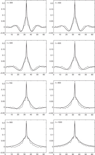
We see that the first estimate of R captures the true covariance well. Considering the estimates at each of the times plotted we see that the true covariance is well approximated. The ETKF with R estimation gives a good estimate of a slowly time-varying observation error covariance matrix. As the covariance is estimated using the innovations from the previous N ^s =250 assimilations we expect to see some delay in the covariance function estimate. We see this in Fig. 2 as the estimated covariance function has a slightly shorter length scale than the true covariance function. This delay could be reduced by reducing the number of samples used. However, this may introduce more sampling error into the estimate of the covariance function.

So far we have shown that it is possible to use the ETKF and DBCP diagnostic to estimate a time-varying observation error covariance matrix. We have shown that it is better to use the ETKFR and an estimated observation error covariance matrix in place of assuming a diagonal matrix. However, if the observation frequency is low, the performance of the ETKFR and the DBCP diagnostic may be reduced.

4.3. Robustness of the ETKFR

We now consider how robust the ETKFR is when we change the covariance used to determine the observation error covariance matrix and how it varies in time. We also consider what happens when observation and background error variances are altered. We run experiments using only the ETKFR and observations are available every five time steps for the Lorenz '96 model and 40 time steps for the KS model. We present results for both the Lorenz '96 and KS experiments in Table 2.

4.3.1. Covariance structures.

We begin by returning to a static matrix but use different length scales to those used in Experiments 3L and 3K. To define the true observation error covariance matrix, R ^t , we use the SOAR function as described by eq. (15) with b=5.0 for experiment 9L and b=3.5 for experiment 9K. With these values of b, the length scale of the observation error covariance is similar to the length scale of the background error covariance. We set the true forecast, correlated and uncorrelated observation error variances to , and the initial matrix used in the assimilation to . We show the results in Table 2. From E1 and E2 we see that the assimilation does not perform as well as the case where the observation error length scales are longer (3L and 3K). From C1 and C2 we see that for 9L the covariance is estimated as well as for 3L. For 9K the estimate of the covariance is only slightly less accurate than 3K. This suggests that the method still works well when the length scales in the observation error covariance matrix are similar to the background error length scales. We conjecture that the good performance of the diagnostic is a result of the background error covariance matrix being accurately evolved by the ETKF.

We now consider the case where the observation error is time varying and the observation error covariance length scale decreases with time. The results are shown in Table 2, Experiments 10L and 10K. In both experiments the assimilation performs well with error metric E2 being similar to Experiments 8L and 8K. C1 and C2 show that the covariance is not estimated quite so well as when the length scales increase with time (Table 1, Experiments 8L and 8K).

In Experiments 11L and 11K, we consider the case where the covariance function used to determine R ^t varies more quickly with time. In this case averaging over the N ^s innovation samples results in an estimated covariance function that has a greater delay than that seen where the covariance function length scale varies more slowly. Again we see the filter is performing well. We find that for Experiment 11L the covariance is well estimated and closely resembles the truth. For Experiment 11K the estimate of the covariance is not as accurate as in the case where the true covariance function varies more slowly with time (8K). However, the variance is well estimated and the correlation length scale is approximately correct (not shown).

4.3.2. Error variances.

We now consider how well the method performs when the magnitudes and ratios of the forecast, uncorrelated and correlated error variances are varied. Experiments 12L, 12K, 13L, 13K, 14L, 14K, 15L and 15K use the time-varying observation error covariance matrix used in Experiments 8L and 8K.

In Experiments 12L and 12K we set the background, , uncorrelated, , and correlated, , error variances to 0.01. In this case, due to the accurate observations and the perfect model assumption, the assimilation performs significantly better than where the error variances were chosen to be 0.1 (8L and 8K). We also find that the observation error covariance is very well estimated with the error undetectable at the level of significance shown.

In Experiments 13L and 13K all the error variances are set to 1. In Experiments 14L and 14K the correlated and uncorrelated observation error variances are set to 1 and the background error covariance is set to 0.1. In each of these experiments, we see a degradation in the analysis. This is due to the large error in the observations. Despite the degradation in the analysis, the percentage of error in the covariance is similar to the cases with other error variances.

Finally in Experiments 15L and 15K we set the initial background error variance to 1, and the observation error variances to 0.1. In these cases the analysis accuracy is similar to Experiments 8L and 8K and the covariance is estimated well.

These experiments suggest that although the initial magnitudes and ratio of the forecast and observation errors may affect the accuracy of the analysis, they do not affect the ability of the ETKFR to estimate the observation error covariance.

5. Conclusions

For a data assimilation scheme to produce an optimal estimate of the state, the error covariances associated with the observations and background must be well understood and correctly specified. As the observation errors have previously been found to be correlated and time-dependent, it is important to determine if the observation error covariance matrix, R, can be estimated within an assimilation scheme. In this work, we introduce an ETKF with observation error covariance matrix estimation. This is an ETKF where analysis and background innovations are calculated at each analysis step and the most recent set of these innovations is used to estimate the matrix R using the DBCP diagnostic. This estimate of R is then used in the next assimilation step. The method has been developed to allow a slowly time-varying estimate of the observation error covariance matrix to be calculated.

In a simple framework, using simple models and neglecting model error we show that estimating R within the ETKF works well, with good estimates obtained, the ensemble spread maintained and the analysis improved in comparison with the case where the matrix R is always assumed diagonal. We also show that the method does not work as well in the case where the observations are less frequent, although this may be dependent on the model. However, the method still produces a reasonable estimate of R, maintains the ensemble variance and the time-averaged error in the analysis is lower than where a diagonal R is used. The method also performs well where the length scale of the observations is similar to the background error length scale.

As we are testing the feasibility of the proposed method, here we consider an isotropic and homogeneous observation error covariance. In practice it is likely that the observation error covariance structure will be non-uniform. As the DBCP diagnostic has previously been successfully used to estimate non-isotropic inter-channel error correlations, for example, Stewart et al. (2014), we would expect the method to be able to estimate a non-uniform observation error covariance matrix but an alternative covariance regularisation method might be required.

We next consider a case where R varies slowly with time. We show that the method works well where the true R is defined to slowly vary with time. The time-averaged error in the analysis is low and the ensemble spread is maintained. The estimates of the covariance matrix are good, suggesting that the method is capable of estimating a slowly time-varying observation error covariance matrix. A case where the length scale of the observation error covariance varies more quickly is also considered, and the ETKFR produces reasonable estimates of the observation error covariance matrix. We also show that the ability of the method to approximate the covariance structure is not sensitive to the forecast error variances or the true magnitude of the observation error variance. Particularly, in the case where observation error variances are increased, the percentage of the error in the covariance is similar to the cases with other error variances despite a degradation in the analysis. This suggests that the method would be suitable to give a time-dependent estimate of correlated observation error. We note that the effectiveness of the method will depend on how rapidly the synoptic situation and hence correlated error is changing and how often observations are available. The correlated error will also be dependent on the dynamical system. For models designed to capture rapidly developing situations, where representativity error and hence correlated error is likely to change rapidly, assimilation cycling and observation frequency within the assimilation is expected to be more frequent and hence more data is available for estimating the observation error.

In this study, the method has been tested under a simplified framework with a perfect model, linear observation operator and assuming that observation errors are isotropic and homogeneous. Many of these simplifying assumptions may not be applicable in an operational framework and further work is required to understand the limitations of the method when these assumptions are violated. In particular, it will be necessary to understand the interaction between the observation error covariance estimation in the ETKFR and the methods of inflation and localisation that will be required when a reduced ensemble size is required. It will also be important to understand how the method performs when the observation error matrix is large and non-isotropic. However, the use of the DBCP diagnostic by Bormann and Bauer (2010), Bormann et al. (2010), Stewart et al. (2009), Stewart (2010), Stewart et al. (2014), Weston (2011), Weston et al. (2014) has been successful in diagnosing correlated observation error covariances, including time invariant non-isotropic inter-channel error correlations, in complex operational models using variational assimilation techniques.

In this study, we have shown that, using the ETKFR, it is possible to estimate time-varying correlated error statistics. However, further work is required to understand the robustness of the ETKFR in an operational framework.

6. Acknowledgements

This work was funded by the European Space Agency (ESA) and the NERC National Centre for Earth Observation (NCEO) and by the Met Office through a CASE studentship. We also thank the three anonymous reviewers whose comments were greatly appreciated. The ETKFR code is available at www.esa-da.org.

References

- Anderson J. L . An ensemble adjustment Kalman filter for data assimilation. Mon. Weather Rev. 2001; 129: 2884–2903.
- Bannister R. N . A review of forecast error covariance statistics in atmospheric variational data assimilation. I: characteristics and measurements of forecast error covariances. Q. J. Roy. Meteorol. Soc. 2008; 134: 1951–1970.
- Bickel P. J. , Levina E . Regularized estimation of large covariance matrices. Ann. Stat. 2008; 36: 199–227.
- Bishop C. , Etherton B. , Majumdar S . Adaptive sampling with the ensemble transform Kalman filter. Part I: theoretical aspects. Mon. Weather Rev. 2001; 129: 420–436.
- Bishop C. H. , Hodyss D . Ensemble covariances adaptively localized with ECO-RAP. Part 1: tests on simple error models. Tellus A. 2009; 61: 84–96.
- Bormann N. , Bauer P . Estimates of spatial and interchannel observation-error characteristics for current sounder radiances for numerical weather prediction. I: methods and application to ATOVS data. Q. J. Roy. Meteorol. Soc. 2010; 136: 1036–1050.
- Bormann N. , Collard A. , Bauer P . Estimates of spatial and interchannel observation-error characteristics for current sounder radiances for numerical weather prediction. II: application to AIRS and IASI data. Q. J. Roy. Meteorol. Soc. 2010; 136: 1051–1063.
- Bormann N. , Saariene S. , Kelly G. , Thepaut J . The spatial structure of observation errors in atmospheric motion vectors from geostationary satellite data. Mon. Weather Rev. 2002; 131: 706–718.
- Buehner M . Lahoz W. , Khattatov B. , Mènard R . Error statistics in data assimilation: estimation and modelling. Data Assimilation Making Sense of Observations .
- Buehner M. , Houtekamer P. , Charette C. , Mitchell H. , He B . Intercomparison of variational data assimilation and the ensemble Kalman filter for global deterministic NWP. Part II: one-month experiments with real observations. Mon. Weather Rev. 2010; 138: 1567–1586.
- Clayton A. M. , Lorenc A. C. , Barker D. M . Operational implementation of a hybrid ensemble/4D-Var global data assimilation system at the Met Office. Q. J. Roy. Meteorol. Soc. 2013; 139(675): 1445–1461.
- Cox S. M. , Matthews P. C . Exponential time differencing for stiff systems. J. Comput. Phys. 2000; 176: 430–455.
- Daley R . Atmospheric Data Analysis. 1991; Cambridge: Cambridge University Press.
- Desroziers G. , Berre L. , Chapnik B . Objective validation of data assimilation systems: diagnosing sub-optimality. Proceedings of ECMWF Workshop on Diagnostics of Data Assimilation System Performance. 2009; 15–17. June 2009.
- Desroziers G. , Berre L. , Chapnik B. , Poli P . Diagnosis of observation, background and analysis-error statistics in observation space. Q. J. Roy. Meteorol. Soc. 2005; 131: 3385–3396.
- Dormand J. , Prince P . A family of embedded Runge-Kutta formulae. J. Comput. Appl. Math. 1980; 6: 19–26.
- Eguíluz V. M. , Alstrøm P. , Hernández-García E. , Piro O . Average patterns of spatiotemporal chaos: a boundary effect. Phys. Rev. E. 1999; 59: 2822–2825.
- Evensen G . The ensemble Kalman filter: theoretical formulation and practical implementation. Ocean Dyn. 2003; 53: 343–367.
- Fertig E. J. , Harlim J. , Hunt B. R . A comparative study of 4D-VAR and a 4D ensemble Kalman filter: perfect model simulations with Lorenz-96. Tellus A. 2007; 59: 96–100.
- Golub G. H. , Van Loan C. F . Matrix Computations. 1996; Baltimore: The Johns Hopkins University Press. 3rd ed.
- Gustafsson J. , Protas B . Regularization of the backward-in-time Kuramoto-Sivashinsky equation. J. Comput. Appl. Math. 2010; 234: 398–406.
- Hamill T. M . Interpretation of rank histograms for verifying ensemble forecasts. Mon. Weather Rev. 2000; 129: 550–560.
- Hamill T. M. , Whitaker J. S. , Snyder C . Distance-dependent filtering of background error covariance estimates in an ensemble Kalman filter. Mon. Weather Rev. 2001; 129: 2776–2790.
- Healy S. B. , White A. A . Use of discrete Fourier transforms in the 1D-Var retrieval problem. Q. J. Roy. Meteorol. Soc. 2005; 131: 63–72.
- Hilton F. , Atkinson N. C. , English S. J. , Eyre J. R . Assimilation of IASI at the Met Office and assessment of its impact through observing system experiments. Q. J. Roy. Meteorol. Soc. 2009; 135: 495–505.
- Hollingsworth A. , Lönnberg P . The statistical structure of short-range forecast errors as determined from radiosonde data. Part I: the wind field. Tellus A. 1986; 38: 111–136.
- Houtekamer P. L. , Mitchell H. L . Ensemble Kalman filtering. Q. J. Roy. Meteorol. Soc. 2005; 133: 3260–3289.
- Janjic T. , Cohn S. E . Treatment of observation error due to unresolved scales in atmospheric data assimilation. Mon. Weather Rev. 2006; 134: 2900–2915.
- Jardak M. , Navon I. M. , Zupanski M . Comparison of sequential data assimilation methods for the Kuramoto-Sivashinsky equation. Int. J. Numer. Meth. Fluid. 2010; 62: 374–402.
- Kassam A. , Trefethen L . Fourth-order time-stepping for stiff PDEs. SIAM J. Sci. Computing. 2005; 25: 1214–1233.
- Kuramoto Y . Diffusion-induced chaos in reaction systems. Prog. Theor. Phys. 1978; 64: 346–367.
- Li H. , Kalnay E. , Miyoshi T . Simultaneous estimation of covariance inflation and observation errors within an ensemble Kalman filter. Q. J. Roy. Meteorol. Soc. 2009; 128: 1367–1386.
- Livings D. M. , Dance S. L. , Nichols N. K . Unbiased ensemble square root filters. Phys. D. 2008; 237: 1021–1028.
- Lorenz E . Predictability: a problem partly solved. Predictability. Proceedings of the 1995. ECMWF Seminar. 1996; 1–18.
- Lorenz E. , Emanuel K . Optimal sites for supplementary weather observations: simulations with a small model. J. Atmos. Sci. 1998; 55: 399–414.
- Mènard R. , Yang Y. , Rochon Y . Convergence and stability of estimated error variances derived from assimilation residuals in observation space. Proceedings of ECMWF Workshop on Diagnostics of Data Assimilation System Performance. 2009; 15–17. June 2009.
- Miyoshi T. , Kalnay E. , Li H . Estimating and including observation-error correlations in data assimilation. Inverse Probl. Sci. Eng. 2013; 21: 387–398.
- Miyoshi T. , Sato Y. , Kadowaki T . Ensemble Kalman filter and 4D-Var intercomparison with the Japanese operational global analysis and prediction system. Mon. Weather Rev. 2010; 138: 2846–2866.
- Ott E. , Hunt B. , Szunyogh I. , Zimin A. , Kostelich E. , co-authors . A local ensemble Kalman filter for atmospheric data assimilation. Tellus A. 2004; 56: 415–428.
- Protas B . Adjoint-based optimization of PDE systems with alternative gradients. J. Comput. Phys. 2008; 227: 6490–6510.
- Sivashinsky G . Non-linear analysis of hydrodynamic instability in laminar flames. Acta Astronautica. 1977; 4: 1177–1206.
- Stewart L. M. PhD Thesis, University of Reading. Correlated Observation Errors in Data Assimilation. 2010. Online at: http://www.reading.ac.uk/maths-and-stats/research/theses/maths-phdtheses.aspx.
- Stewart L. M., Cameron J., Dance S. L., English S., Eyre J. R., co-authors. Technical report, University of Reading. Mathematics reports series. Observation Error Correlations in IASI Radiance Data. 2009. Online at: http://www.reading.ac.uk/web/FILES/maths/obs_error_IASI_radiance.pdf.
- Stewart L. M. , Dance S. L. , Nichols N. K . Correlated observation errors in data assimilation. Int. J. Numer. Meth. Fluid. 2008; 56: 1521–1527.
- Stewart L. M. , Dance S. L. , Nichols N. K . Data assimilation with correlated observation errors: experiments with a 1-D shallow water model. Tellus A. 2013; 65: 19546.
- Stewart L. M. , Dance S. L. , Nichols N. K. , Eyre J. R. , Cameron J . Estimating interchannel observation-error correlations for IASI radiance data in the Met Office system. Q. J. Roy. Meteorol. Soc. 2014; 140: 1236–1244.
- Thiebaux H . Anisotropic correlation functions for objective analysis. Mon. Weather Rev. 1976; 104: 994–1002.
- Waller J. A. PhD Thesis, Department of Mathematics and Statistics, University of Reading. Using Observations at Different Spatial Scales in Data Assimilation for Environmental Prediction. 2013. Online at: http://www.reading.ac.uk/maths-and-stats/research/theses/maths-phdtheses.aspx.
- Waller J. A. , Dance S. L. , Lawless A. S. , Nichols N. K. , Eyre J. R . Representativity error for temperature and humidity using the Met Office high-resolution model. Q. J. Roy. Meteorol. Soc. 2014; 140: 1189–1197.
- Weston P . Technical report, Met Office, UK. Progress Towards the Implementation of Correlated Observation Errors in 4D-Var. 2011. Forecasting Research Technical Report 560.
- Weston P. P. , Bell W. , Eyre J. R . Accounting for correlated error in the assimilation of high resolution sounder data. Q. J. Roy. Meteorol. Soc. 2014. Early View.
- Whitaker J. S. , Hamill T. M. , Wei X. , Song Y. , Toth Z . Ensemble data assimilation with the NCEP global forecast system. Mon. Weather Rev. 2008; 136: 463–482.
- Wilks D. S . Statistical Methods in the Atmospheric Sciences. 1995; San Diego: Academic Press.