Pattern decomposition of the transient climate response

Abstract

A two-pattern decomposition of the mean surface air temperature response to an increase of CO₂ is assessed. This decomposition is based on a two-layer global energy-balance model and the hypothesis of separability in space and time. It is shown that this decomposition allows the regional transient warming of a given atmosphere–ocean general circulation model to be well represented. The pattern decomposition is applied to 16 CMIP5 climate models and each of the two retrieved patterns – the equilibrium pattern and the pattern associated with the deep-ocean heat uptake – is described and discussed.

• transient regional response
• pattern scaling
• energy balance model
• climate sensitivity
• ocean heat uptake

To access the supplementary material to this article, please see Supplementary files under Article Tools online

1. Introduction

Energy-balance models (EBM) can be used to emulate the global-mean surface-air temperature response of a given coupled atmosphere–ocean general circulation model (AOGCM) to an externally imposed radiative perturbation and to analyse the key mechanisms at play in this response. It has been shown that two time scales (and an instantaneous response) resulting from the low inertia of the near-surface ocean and the large inertia of the deep ocean allows a good representation of the main behaviour of the transient response as simulated by climate models, that is, the response of the global surface air temperature is well described by a two-layer energy-balance model (Held et al., 2010; Geoffroy et al., 2013a, 2013b) (thereafter H10, G13a and G13b). Using climate models that participated in the fifth phase of the Coupled Model Intercomparison Project (CMIP5, Taylor et al., 2011), G13a,b show that it is possible to calibrate the parameters of such EBM from an abrupt CO₂ experiment to reproduce the responses to a gradual increase of CO₂.

However, such EBMs allow the response at the global scale to be described, whereas the climate response has a non-uniform geographical structure. The pattern scaling technique has been proposed first to extrapolate a transient regional response from the equilibrium regional response (Santer et al., 1990). This method has then been used to represent the response of temperature or other variables to a wide range of greenhouse gas emissions scenarios (e.g. Mitchell et al., 1999; Harris et al., 2006; Frieler et al., 2012; Ishizaki et al., 2013). These methods rely on one single pattern of decomposition, alternatively with an additional pattern to take into account the aerosol forcing (e.g. Schlesinger et al., 2000).

The use of one single pattern may be limited to represent scenarios with forcings of significantly different amplitude (Huntingford and Cox, 2000), stabilisation and long-term integration (Mitchell, 2003). Indeed, the equilibrium and the transient regional temperature responses are characterised by different typical patterns that have been investigated in the literature (Manabe and Stouffer, 1980; Manabe et al., 1991). By analysing a particular AOGCM and using an instantaneous abrupt return to preindustrial forcing, H10 highlight a two-pattern decomposition of the transient temperature response and discuss structural differences between the fast and the slow components of the regional response. Their results suggest that an EBM framework combined with a two-pattern decomposition could be used to emulate the regional transient climate response (TCR).

The purpose of this article is to investigate the validity of an EBM time–space decomposition in predicting the regional climate response for any AOGCM and any CO₂ increase scenario. The decomposition used in this study is presented in Section 2 and validated in Section 3 by using CMIP5 1% yr⁻¹ CO₂ experiments. In Section 4, the two patterns resulting from the decomposition are described and discussed for the CMIP5 AOGCMs studied.

2. Framework and method

2.1. Decomposition of the global response

Within the framework of the two-layer EBM described in H10 and G13a,b, the heat content change of the upper layer is expressed as1

where is the adjusted radiative forcing, the deep-ocean heat uptake, the global-mean surface air temperature response, λ the equilibrium radiative response parameter and ɛ the efficacy factor of deep-ocean heat uptake. Each term in eq. (1) represents a global-mean quantity (denoted by an overline). The sum represents the radiative response of the climate system.

Equation (1) can be rewritten noting that the global-mean surface air temperature response is the sum of an equilibrium mean surface air temperature response associated with the adjusted radiative forcing and two mean surface air temperature responses and associated with the upper- and the deep-ocean heat content changes, respectively:2

with3 4 5

The radiative response parameter associated with the deep-ocean heat uptake, λ _D =λ/ɛ, is different from the equilibrium global radiative response parameter λ because the pattern of the response is different from that of equilibrium and because feedbacks vary geographically (Winton et al., 2010). The different nature of the ‘forcings’ (the radiative forcing and the deep-ocean heat uptake) at play may also be a cause of difference in the strength of the feedbacks.

The analytical solutions of and for an abrupt forcing and a linear forcing (i.e. a 1% yr⁻¹ CO₂ experiment) scenarios are given in G13b (see also their Fig. 1). It is noteworthy that the amplitude of is small after several years for an abrupt CO₂ forcing or for a gradually increasing forcing. Therefore, most of the deviation from the equilibrium response is due to (i.e. due to the deep-ocean heat uptake).

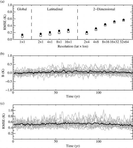
Fig. 1 Multimodel mean and temporal mean (over the 70–140 yr period) of RMSE(t) (solid circles) and RMS _ctl (t) (squares) for different spatial resolutions (a) and temporal evolution for individual AOGCM values (grey lines) and multimodel mean (thick line) of the bias B(t) (b) and the root-mean-square error RMSE(t) (c) for the 16×32 grid.

2.2. Pattern decomposition

Following G13b, we assume that the regional temperature response ΔT(x, t) is the sum of the three regional responses ΔT _eq (x, t), ΔT _U (x, t) and ΔT _D (x, t) associated with , and , respectively:6

where x is the horizontal coordinate of a given region and the quantity ΔT(x, t) is the average of the local temperature response over this region.

Then, by assuming separability in space and time (Hasselmann, 1993), each regional temperature response is expressed as the product of a space-dependent function (pattern function) and the corresponding time-dependent global-mean surface air temperature change. The formulation of the two-layer EBM imposing that the pattern associated with the upper-ocean heat uptake is equal to the equilibrium pattern [note that this equality is imposed by the initial conditions in the case of a step forcing (G13b)], the regional temperature response reads:7

where r _eq (x) is the equilibrium pattern function and r _D (x) is the pattern function associated with the deep-ocean heat uptake. These functions give the normalised spatial amplitude of the warming associated with the adjusted radiative forcing (in equilibrium) and with the deep-ocean heat uptake. In this framework, the transient spatial warming is the sum of the homothetic transformation of r _eq (x) and that of r _D (x) of scale factor and , respectively.

2.3. Method for determining the pattern functions

The parameters of the EBM are derived following the calibration method described in G13a,b. This method is based on linear (and multilinear) regressions using the time evolution of the global mean temperature response and of the radiative imbalance. For each individual AOGCM, the values of the EBM parameters are obtained using the annual mean temperature change of the abrupt 4×CO₂ experiment over the 150-yr period with respect to the temporal mean value of the control simulation over the same period. The analytical EBM responses , and are then calculated according to G13b.

At each grid cell of coordinate x, and for each individual AOGCM, the values of the pattern functions r _eq (x) and r _D (x) are determined by a multiple linear regression of the regional surface air temperature change of the climate model abrupt 4×CO₂ experiment against the EBM analytical global responses and , respectively (see eq. 7). Note also that the first point of the regression (t=0) is associated with a large weight (and s set to zero) in order to ensure that the intercept of each regression [and thus ΔT(x, 0)] is zero.

The method is applied to the 16 AOGCMs of the CMIP5 analysed in G13b.

3. Validation of the pattern decomposition

3.1. Method for validation

To evaluate the time–space decomposition of the TCR described above, we compare the climate model regional response in the 1% yr⁻¹ CO₂ experiment (that has not been used for calibration) to the corresponding predicted regional response ΔT(x, t). For each AOGCM, ΔT(x, t) is calculated from eq. (7) with the EBM parameters and the pattern functions derived from the 4×CO₂ experiment.

To compare the AOGCM spatial pattern of the transient response to the EBM predicted response, we first consider (Section 3.2) two global mean metrics, the spatial mean of the regional bias:8

and the root-mean-square error (RMSE) of the spatial response:9

where n _x is the number of grid points. The RMSE can be compared to the root-mean-square of the surface air temperature anomaly ΔT _ctl in the pre-industrial control experiments10

which gives a measure of the spatial variability due to internal variability. Note that these quantities are calculated using annual mean values.

As a second step (Section 3.3), we compare the spatial pattern of the TCR. The results presented will focus on the multimodel mean of these quantities. The individual model results are plotted in the Supplementary file. Note that over the 16 climate models studied, 15 are used in the multimodel analysis. The INM climate model is excluded because it is an outlier for the deep ocean specific heat capacity (G13a). This may be due to the fact that it is characterised by a cooling of the northern hemisphere during the slow part of the temperature evolution (after 30 yr) of the abrupt experiment.

3.2. Sensitivity to the resolution

In order to investigate to what spatial extent the hypothesis of time–space separability remains valid, the method is applied to different spatial resolutions, including latitudinal grids with 2, 4, 8, 16 bands of latitudes and latitude–longitude grids with 2×4, 4×8, 8×16, 16×32 and 32×64 grid cells. Note that for all resolutions, we use grid cells of equal area.

Figure (1a) represents the multimodel mean and temporal mean over years 70–140 of RMSE(t) and RMS _ctl (t) for grids of the different resolutions listed above. As expected, the error increases for finer spatial resolutions. However, for all resolutions, the error is close to RMS _ctl (t), indicating that most of the regional biases are due to internal variability. Thus, the framework captures the regional transient temperature response for all resolutions. Hereafter, the resolution 16×32 is used.

The temporal evolution of the multimodel mean of B(t) and of the multimodel mean of RMSE(t) are shown in Fig. 1b, c (thick lines). Each individual model value is also represented (grey lines). The global-mean of the regional bias is equal to the bias of the global temperature response (by construction). During the first years, the warming is small: the bias is close to zero and the error is close to that obtained with natural variability. Both B(t) and RMSE(t) remain small during the following 140 yr of warming, indicating a good representation of the regional temperature response.

The bias and the RMSE slightly increase over the first half of the 140 yr and slightly decrease over the second half of the period as is the case at the global scale (see Fig. 2 in G13a). This may be due to the lack of intermediate time scales in the two-layer EBM, as pointed by Merlis et al. (2013). The decrease of both the bias and the error during the second half of the experiment may be fortuitous or may be due to the fact that the EBM is calibrated using the abrupt 4×CO₂ simulation. Thus, the parameters, such as the adjusted forcing and the radiative response parameter, may be better suited to representing 4×CO₂ conditions. Indeed, the assumption of perfect logarithmic dependence between the adjusted forcing and the CO₂ concentration may be limited or the radiative response parameter may vary slightly with the climate state.

Fig. 2 (Left) Multimodel mean of the AOGCM regional transient temperature response TCR (mean over the period 55–85 yr of the 1% yr⁻¹ CO₂ experiment). (Middle) Mean of the corresponding regional temperature responses as predicted by the EBM calibrated with the AOGCM abrupt experiment, and the difference between the two (right).

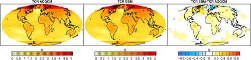
3.3. Regional TCR

We now compare the geographical distribution of the TCR (defined here as a 31-yr mean response centred over the year 70, that is, the time of 2×CO₂) of the multimodel AOGCMs to that predicted by the EBM time–space decomposition. Figure 2 shows both regional responses and their differences. The main features of the TCR, North–South hemisphere dissymmetry, Arctic polar amplification, enhanced lands warming and strongly delayed warming in southern oceans (Manabe et al., 1991; H10), are well reproduced by the EBM time–space decomposition estimation.

For individual models (Fig. S1), the differences between the AOGCM response and the EBM-predicted response exhibit larger spatial disparities, partly because the effect of internal variability is enhanced by the use of only one single member per climate model. However, the spatial distributions are generally in good agreement, even in regions where the response differs from one model to another. It is also interesting to note that in regions where abrupt experiments show a slow cooling, the 1% yr⁻¹ CO₂ response is well reproduced, with values at the end of the 1% yr⁻¹ CO₂ potentially larger than those of the abrupt 4×CO₂, as predicted by the EBM estimation (not shown).

The North Atlantic Ocean constitutes the main region of bias. Indeed, for most of the AOGCMs, in the abrupt 4×CO₂ experiment, the temperature response exhibits a non-linear behaviour in this region (not shown) possibly due to the response of the Atlantic meridional overturning circulation (H10; Ishizaki et al., 2012). The land surfaces are also an important region of differences.

Note that the use of one single pattern in eq. 5 leads to similar results, with a slight increase of the error in the southern circumpolar ocean (see Fig. S2). This confirms previous studies, that, given an adequate representation of the global temperature response, a single pattern decomposition is able to represent the regional temperature response. However, some studies also suggest that for scenario with significantly different forcing amplitude, the use of a single pattern may be limited (Huntingford and Cox, 2000). A single pattern decomposition may also fail to represent a long-term simulation such as a stabilisation, the pattern in equilibrium being different from the transient pattern (Mitchell et al., 1999; Mitchell, 2003). The two-pattern decomposition described in this article should counteract these limitations by distinguishing the pattern associated with the radiative forcing and that associated with the deep-ocean heat-uptake. These two patterns are presented in next section for the CMIP5 AOGCM ensemble.

4. Pattern functions

4.1. Equilibrium pattern

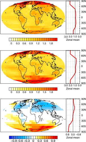
Figure 3 shows the multimodel mean of the patterns and . The pattern associated with the adjusted radiative forcing equilibrium exhibits well-documented spatial structures. The enhanced warming over lands and the polar amplification in both hemispheres (Manabe and Stouffer, 1980; Manabe et al., 1991) are a robust pattern in the climate models (except for the INM climate model). Whereas the Arctic amplification is pronounced for all models, the relative amplitude of the polar amplification varies from one model to another. Further, the results suggest a negative equilibrium temperature response in the North Atlantic region for some AOGCMs (Fig. S3). However, the time–space decomposition framework is limited in this region, as noted previously. The robustness of the equilibrium pattern is confirmed by the low values of the intermodel standard deviation of r _eq (x) (see Fig. S4).

Fig. 3 Multimodel mean of the pattern functions (top), (middle) and their difference (bottom). The corresponding zonal mean is also shown for each pattern (red line, right panels).

Due to the larger time scales involved, the EBM estimation of the equilibrium pattern may differ from the real equilibrium pattern of the climate model. In particular, the southern circumpolar ocean current slows down the warming at the millennial time scale and may impact the strength of the feedbacks after several centuries of simulation (e.g. Li et al., 2012). In such a case, r _eq (x) has to be considered as an apparent equilibrium pattern, providing justification for the representation of the transition at the centennial scale.

4.2. Pattern associated with deep-ocean heat uptake

In transition, the surface air temperature pattern is a combination of r _eq (x) and the pattern associated with the deep-ocean heat uptake r _D (x). At a time t, the contribution of each pattern depends on the amplitude of the adjusted radiative forcing and of the history of the warming. Because the contribution of the upper-ocean is small in comparison to that of ( , except during the first years for an abrupt forcing case), the component projected on r _eq (x) increases roughly linearly with the forcing, and most of the deviation from the instantaneous equilibrium response is projected over r _D (x). Since is negative, regions where r _D (x) is greater than one represent a lower warming relative to that of equilibrium and a larger warming for regions where r _D (x) is lower than one. For a stabilisation or an abrupt forcing, is constant and increases until zero: the spatial distribution of the surface air temperature tends towards the equilibrium temperature distribution.

Whereas the decomposition presented here differs from that described in H10, the pattern r _D (x) is similar to the pattern of their recalcitrant component of global warming, highlighted by performing an abrupt return to preindustrial conditions. Indeed, when the forcing is set instantaneously to zero, decreases rapidly until zero, quickly changes sign and decreases slowly. As a result, after few years, the regional temperature change is with .

The multimodel mean of the pattern associated with the deep-ocean heat uptake r _D (x) and the multimodel mean of the difference between r _D (x) and r _eq (x) are shown in Fig. 3. The results for each individual AOGCM are shown in Fig. S3. The results show a good agreement with the pattern of the recalcitrant component of global warming of H10. It is interesting to note that their pattern is similar to that of the GFDL model (see Fig. 7 of H10 and Fig. S3). The pattern of r _D is relatively similar to the pattern of r _eq . If the patterns were equal, it would mean that the deep-ocean heat uptake slows down the warming everywhere in the same proportion relatively to the equilibrium pattern.

Some differences can be observed in particular regions. Whereas the warming is particularly delayed in the southern circumpolar ocean (Manabe et al., 1991), it is relatively larger over lands during the transition (H10). As discussed in H10, the warming is also delayed in the ENSO region for most of the AOGCMs (r _D is larger than 1 for 11 models) and in the multimodel mean. Some models exhibit negative values of r _D , mainly in the North Atlantic Ocean. As mentioned previously, the EBM decomposition appears not to be not adapted to this region.

The intermodel standard deviation of the pattern r _D is larger than that of r _eq (not shown). However r _D is associated with a temperature response of a lower magnitude than and the intermodel spread of r _eq is small. Thus one may expect that the intermodel differences of the patterns contribute less to the spread of the regional temperature response than the difference between the global temperature responses. This question may be assessed by performing an ANOVA (e.g. Geoffroy et al., 2012) by considering the patterns and the global mean temperature response as variables.

5. Conclusion and perspective

In this article, we have shown that within an energy-balance framework, and by using the assumption of separability in space and time, we can derive a two-pattern decomposition that gives a good representation of the transient regional climate response to a gradual CO₂ increase with a calibration from an abrupt experiment only. The method has been validated by using 16 CMIP5 climate models. The main geographical features (over the southern circumpolar ocean and the land areas) of the temperature response are well reproduced within this method. The retrieved patterns are in very good agreement with previous studies (H10). The main limitations of the EBM time–space decomposition concern the North Atlantic Ocean and land areas, highlighting some deficiencies of the EBM framework. The reason for such discrepancies should be investigated. This decomposition may be valid for all type of scenario, including stabilisation and long-term simulations. Moreover, the results have highlighted some outliers in the 16 CMIP5 models such as the INMCM4 climate model (and to a lesser extent FGOALS-s2 and CNRM-CM5 climate models) that shows a negative sensitivity to the heat uptake in most of the North Hemisphere.

The use of two patterns should allow us to predict the regional temperature response for all kinds of greenhouse gas scenario at the centennial to the millennial scale. The derived patterns could also be used as inputs for SSTclim experiments to study the radiative response in equilibrium and transient conditions. Another perspective of this work is to investigate to which extent the response of other variables, such as the precipitation rate, are represented by using such a pattern of decomposition. Moreover, the validity of this framework to other external radiative perturbations (aerosols, solar) and to a combination of external perturbations should be examined. If the use of one single pattern is sufficient in representing the transient response of idealised CO₂ experiments at the scale of few decades, using a one- or a two-pattern decomposition should be assessed for these other types of forcing. Moreover, recent studies show that detection and attribution methods based on temperature response patterns are not able to distinguish the response associated with the 20th century greenhouse gas increase and that associated with the aerosol forcing (Ribes and Terray, 2013). A decomposition like the one presented here could be used to help study the differences in the pattern response associated with these forcings. Thus, applications to climate sensitivity constraints or detection and attribution studies could be envisaged.

6. Acknowledgements

We thank the anonymous reviewers whose comments and suggestions helped to improve the manuscript. Aurélien Ribes and Hervé Douville are also thanked for helpful discussions. We acknowledge the World Climate Research Programme's Working Group on Coupled Modelling, which is responsible for CMIP, and the US Department of Energy's Program for Climate Model Diagnosis and Intercomparison, which provides coordinating support and leads the development of software infrastructure in partnership with the Global Organization for Earth System Science Portals. We thank the climate modelling groups for producing and making available their model output. This work was supported by the European Union FP7 Integrated Project COMBINE.

Notes

To access the supplementary material to this article, please see Supplementary files under Article Tools online

The 16 models analysed are BCC-CSM1-1, BNU-ESM, CanESM2, CCSM4, CNRM-CM5, CSIRO-Mk3.6.0, FGOALS-s2, GFDL-ESM2M, GISS-E2-R, HadGEM2-ES, INMCM4, IPSL-CM5A-LR, MIROC5, MPI-ESM-LR, MRI-CGCM3 and NorESM1-M, for which the values of the EBM parameters are provided in Tables 1 and 2 of G13b.

References

- Frieler K. , Meinshausen M. , Mengel M. , Braun N. , Hare W . A scaling approach to probabilistic assessment of regional climate change. J. Clim. 2012; 25: 3114–3144.
- Geoffroy O. , Saint-Martin D. , Bellon G. , Voldoire A. , Olivié D. J. L. , co-authors. Transient climate response in a two-layer energy-balance model. Part II: representation of the efficacy of deep-ocean heat uptake and validation for CMIP5 AOGCMs. J. Clim. 2013b; 26: 1859–1876.
- Geoffroy O. , Saint-Martin D. , Olivié D. J. L. , Voldoire A. , Bellon G. , co-authors. Transient climate response in a two-layer energy-balance model. Part I: analytical solution and parameter calibration using CMIP5 AOGCM experiments. J. Clim. 2013a; 26: 1841–1857.
- Geoffroy O. , Saint-Martin D. , Ribes A . Quantifying the sources of spread in climate change experiments. Geophys. Res. Lett. 2012; 39: L24703.
- Harris G. R. , Sexton D. M. H. , Booth B. B. B. , Collins M. , Murphy J. M. , co-authors. Frequency distributions of transient climate change from perturbed physics ensembles of general circulation model simulations. Clim. Dynam. 2006; 27: 357–375.
- Hasselmann K . Optimal fingerprints for the detection of time-dependent climate change. J. Clim. 1993; 6: 1957–1971.
- Held I. M. , Winton M. , Takahashi K. , Delworth T. , Zeng F. , co-authors. Probing the fast and slow components of global warming by returning abruptly to preindustrial forcing. J. Clim. 2010; 23: 2418–2427.
- Huntingford C. , Cox P. M . An analogue model to derive additional climate change scenarios from existing GCM simulation. Clim. Dynam. 2000; 16: 575–586.
- Ishizaki Y. , Shiogama H. , Emori S. , Yokohata T. , Nozawa T. , co-authors . Temperature scaling pattern dependence on representative concentration pathway emission scenarios. Clim. Change. 2012; 112: 535–546.
- Ishizaki Y. , Shiogama H. , Emori S. , Yokohata T. , Nozawa T. , co-authors. Dependence of precipitation scaling patterns on emission scenarios for representative concentration pathways. J. Clim. 2013; 26: 8868–8879.
- Li C. , von Storch J. S. , Marotzke J . Deep-ocean heat uptake and equilibrium climate response. Clim. Dynam. 2012; 40: 1071–1086.
- Manabe S. , Stouffer R. J . Sensitivity of a global climate model to an increase of CO2 concentration in the atmosphere. J. Geophys. Res. 1980; 85: 5529–5554.
- Manabe S. , Stouffer R. J. , Spelman M. J. , Bryan K . Transient responses of a coupled Ocean–atmosphere model to gradual changes of atmospheric CO2. Part I. Annual mean response. J. Geophys. Res. 1991; 4: 785–818.
- Merlis T. M. , Held I. M. , Stenchikov G. L. , Zeng F . Constraining transient climate sensitivity using coupled climate model simulations of volcanic eruptions. J. Clim. 2013. submitted.
- Mitchell J. F. B. , Johns T. C. , Eagles M. , Ingram W. J. , Davis R. A . Towards the construction of climate change scenarios. Clim. Change. 1999; 41: 547–581.
- Mitchell T. D . Pattern scaling. An examination of the accuracy of the technique for describing future climates. Clim. Change. 2003; 60: 217–242.
- Ribes A. , Terray L . Application of regularised optimal fingerprinting to attribution. Part II: application to global near-surface temperature. Clim. Dynam. 2013; 41: 2837–2853.
- Santer B. D. , Wigley T. M. L. , Schlesinger M. E. , Mitchell J. F. B . Developing climate scenarios from equilibrium GCM results . 1990; Max-Planck Institut fur Meteorologie report, 47. 29.
- Schlesinger M. E. , Malyshev S. , Rozanov E. V. , Yang F. , Andronova N. G. , co-authors. Geographical distributions of temperature change for scenarios of greenhouse gas and sulfur dioxide emissions. Technol. Forecast. Soc. Change. 2000; 65: 167–193.
- Taylor K. E. , Stouffer R. J. , Meehl G. A . An overview of CMIP5 and the experiment design. Bull. Am. Meteorol. Soc. 2011; 93: 485–498.
- Winton M. , Takahashi K. , Held I. M . Importance of ocean heat uptake efficacy to transient climate change. J. Clim. 2010; 23: 2333–2344.