An algorithm based on sea-level pressure fluctuations to identify major Baltic inflow events

Abstract

Major Baltic inflows are an important process to sustain the sensitive steady state of the Baltic Sea. We introduce an algorithm to identify atmospheric variability favourable for major Baltic inflows. The algorithm is based on sea-level pressure (SLP) fields as the only parameter. Characteristic SLP pattern fluctuations include a precursory phase of 30 days and 10 days of inflow period. The algorithm identifies successfully the majority of observed major Baltic inflows between 1961 and 2010. In addition, the algorithm finds some occurrences which cannot be related to observed inflows. In these cases with favourable atmospheric conditions, inflows were precluded by contemporaneously existing saline water masses or strong freshwater supply. Moreover, the algorithm clearly identifies the stagnation periods as a lack of SLP variability favourable for MBIs. This indicates that the lack of inflows is mainly a consequence of missing atmospheric forcing during this period. The only striking inflow which is not identified by the algorithm is the event in January 2003. We demonstrate that this is due to the special evolution of SLP fields which are not comparable with any other event. Finally, the algorithm is applied to an ensemble of scenario simulations. The result indicates that the number of atmospheric events favourable for major Baltic inflows increases slightly in all scenarios.

• major Baltic inflows
• algorithm development
• SLP variability
• Baltic Sea
• climate modeling

1. Introduction

The Baltic Sea is one of world's largest brackish water areas with an estuarine-like circulation. It is connected to the world ocean through the narrow Danish straits limiting the exchange of water masses. The deep water of the Baltic Sea is mainly renewed by so-called major Baltic inflows (MBIs) which are of special importance for the Baltic Sea. They bring salty and oxygen-rich water into the deep basins which have a significant impact on the marine ecosystem. The absence of MBIs especially in combination with anthropogenic eutrophication and climate change lowers oxygen concentrations dramatically turning the deep basins into dead zones (Meier et al., 2012).

A common method to identify MBIs is based on salinity measurements at the Darss Sill (Matthäus and Franck, 1992). Following the method by Matthäus and Franck (1992), an MBI is registered as soon as the bottom salinity at Darss Sill is >17 (g/kg) in combination with a weak stratification for at least five days in a row. MBIs occur intermittently during the winter half year with most events from November to January (Matthäus and Franck, 1992). MBIs are mainly driven by an increase of the zonal wind, which increases on average from 3–4 to 14 m/s over a couple of days (Matthäus and Schinke, 1994). The corresponding sea surface slope into the Baltic Sea leads to a barotropic flow over the Darss and Drogden sills into the Baltic Sea. On average, the water level of the Baltic Sea rises during MBIs by 59 cm which corresponds to a volume of roughly 193 km³ (Matthäus and Franck, 1992).

In general, two phases of an MBI can be separated, the precursory and the inflow period (Matthäus and Franck, 1992). The precursory period covers the time from the minimum Baltic Sea-level preceding a major event to the start of the event at Darss Sill (Matthäus and Schinke, 1994). Hereby, the last 15 days are often referred to as the pre-inflow period which is of great importance for the MBI. The MBI ends with strong outflow due to the weakening of the west wind and the above normal filling of the Baltic (Matthäus and Schinke, 1994).

Sea-level pressure (SLP) patterns related to MBIs are investigated by Matthäus and Schinke (1994) and Schinke and Matthäus (1998). They show positive SLP anomalies over the Baltic Sea 50–20 days prior to the main inflow period. The SLP-pressure gradient starts to increase approximately 10 days before the onset. The maximum SLP gradients are found on the day before and on the first day of the inflow event. Generally, stronger inflows have stronger gradients, which are related to higher wind speeds (Matthäus and Schinke, 1994).

On average, more than one MBI occurs per inflow season. Matthäus and Franck (1992) classified 90 MBIs between 1897 and 1976 between the end of August and the end of April. However, they state also that 26% of the inflow seasons were without any MBI. The period 1976–1992 is characterised by a reduced number of MBIs (Lass and Matthäus, 1996). After the MBI in January 1983, a decade without any major inflow was observed (e.g. Meier et al., 2012). This period is known as the stagnation period and comes with a reduction of deep water salinity and oxygen concentrations.

Reasons for the lack of MBIs during the stagnation period are still debated. Several factors are known to hamper MBIs and are therefore discussed as reasons for the stagnation period. First, stronger outflow counteracts the inflow. So, increased runoff and net precipitation reduces the chance for MBIs (Schinke and Matthäus, 1998; Meier and Kauker, 2003). However, this cannot explain the recent stagnation period completely (Meier and Kauker, 2003). Stronger westerlies are related to lower than normal salinities in the upper and lower layers in all areas of the Baltic Sea (Zorita and Laine, 2000). This is due to related stronger precipitation which raises the sea level in the Baltic (Schinke and Matthäus, 1998) as well as a higher mean filling of the Baltic Sea due to stronger westerlies (Meier and Kauker, 2003; Gräwe et al., 2013). Moreover, west-wind anomalies can change the occurrence of MBIs by additional mixing in the Danish Straits (Gräwe et al., 2013). Lass and Matthäus (1996) argued that the probability of both negative north and negative east components of the wind with duration of more than 10 days was slightly larger during the period of regular inflow events than during the period of reduced inflow from 1976 to 1992.

Gustafsson and Andersson (2001) simulated the occurrences and strengths of large high-saline inflows to the Baltic with the north–south air pressure difference across the North Sea as the only forcing. Moreover, the freshwater outflow of the Baltic is correlated with the mean zonal wind over the Baltic Sea (Hordoir and Meier, 2010). Recently, Hordoir et al. (2013) managed to predict the freshwater outflow with an acceptable accuracy of 70% by using wind data only.

The special meaning of MBIs for the state of the Baltic Sea emphasises the need of understanding trigger mechanisms in more detail as well as exploring natural variability and possible anthropogenic induced change in the number of occurrences. The main idea of this paper is to identify possible occurrences of MBIs using SLP fields as the only predictor. This approach was never applied before. Earlier studies solely showed composites between conditions leading to MBIs and the mean state (e.g. Matthäus and Schinke, 1994; Lass and Matthäus, 1996; Schinke and Matthäus, 1998). Or, they used SLP gradients to simulate inflow events (Gustafsson and Andersson, 2001). We decided to use SLP only since it is the single parameter comprising the most relevant information. Wind speed and direction is directly related to SLP fields via the geostrophic wind approximation. Using SLP fields instead of wind fields implies using one parameter instead of two and by that keeping the complexity as low as possible. Moreover, SLP fields incorporate water pumping between the North Sea and the Baltic Sea due to changes in surface pressure over both seas. Finally, SLP has large scale structures that are simulated more reliable than strongly parameterised 10 m wind speed in climate models.

The paper is organised as follows: Section 2 describes the model and the data. Section 3 investigates mean features of SLP variability related to MBIs and introduces a new algorithm to identify MBIs. In Section 4, the algorithm is first validated and then applied to scenario simulations to identify possible changes in the number of strong MBIs in scenario simulations. The results are summarised and discussed in Section 5.

2. Models and experiments

2.1. The Rossby Centre Atmosphere model

The atmospheric model used for our investigations is the Rossby Centre Atmosphere model version 4 (hereafter referred to as RCA4). It is based on the numerical weather prediction model HIRLAM (Unden et al., 2002). It is applied with a horizontal resolution of 0.22° (approx. 25 km) on a rotated longitude–latitude grid. In the present setup, RCA4 is used with 40 vertical levels and a time step of 15 min. Lateral boundary forcing as well as sea surface temperatures are prescribed from ERA40 (Uppala et al., 2005) whereas lakes are modelled with FLake (Mironov et al., 2010).

The formation of MBIs crucially depends on the precise evolution of SLP-fields. Therefore, a spectral nudging technique was applied for the hindcast simulation to ensure that low pressure systems pass through the model domain as close to observations as possible. The setup uses a nudging strength of 0.1 at the model top, a frequency of once every hour and a minimum wavelength of 800 km.

The reader is referred to Samuelsson et al. (2011) (for a detailed model description and validation of RCA3) and Wang et al. (submitted, in this special issue) where changes from RCA3 to RCA4 are highlighted. For more details regarding the applied spectral nudging, the reader is referred to Berg et al. (2013).

2.2. Experimental setup and data

Model data used for the development of the algorithm are based on a simulation driven with ERA40. The simulation covers the period 1961–2010. Only SLP data are taken from the simulation. Moreover, we use daily averages since a higher resolution in time is not needed to identify MBIs. The horizontal domain includes all of Europe from the Mediterranean Sea to the northern tip of Scandinavia. Herewith, almost the entire RCA4 domain is used neglecting only the relaxation zone at the outer boundary and the southern most part.

Dates of observed MBIs are taken from Matthäus et al. (2008) and updated by R. Feistel (personal communication, October 2013). Moreover, time series of salinity based on measurements are used for the centre of the Bornholm Basin (name of the station is BY5) and the Gotland Deep (BY15). These measurements are freely available in the SMHI data base SHARK (Svenskt HavsARKiv, see http://www.smhi.se/oceanografi/oce_info_data/SODC/overview.htm).

3. Method

3.1. Mean features of SLP pattern variability

To identify the special characteristics of SLP anomalies, 13 observed MBIs are selected (see Table 1). The selected events are chosen based on two criteria: (1) they were supposed to be isolated in time, for example, not in a cluster of two or more events within a period of less than 30 days; (2) they need to be classified at least with a strength of Q=10 according to the method of Fischer and Matthäus (1996). The isolation in time is desired so that there is no overlap between the inflow period of one MBI and the precursory phase of the following event. Moreover, the omission of the weakest MBIs was done to get more robust results.

Table 1. Onset dates of used MBIs and their relative intensity Q

Date	Intensity Q	Date	Intensity Q
1961-03-26	12.7	1970.10.27	15.0
1961-12-02	16.4	1973.11.13	27.0
1963-11-18	13.7	1976.11.30	13.3
1964-02-03	11.0	1982.11.18	12.7
1965-10-30	29.5	1983.01.13	12.0
1969-02-01	13.2	1993.01.18	34.0
1969-10-29	29.2

Data are based on Matthäus and Franck (1992) re-assessed by Fischer and Matthäus (1996) and supplemented and updated by Matthäus (2006).

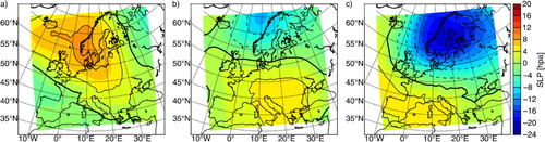
The mean development of SLP fields related to MBIs is presented and discussed by Matthäus and Schinke (1994) and for comparison reasons in Fig. 1. The beginning of the precursory period is in general characterised by positive SLP deviations over Scandinavia and the North Atlantic (Fig. 1a). This is related to an often weak but steady easterly flow, which lowers the sea level of the Baltic Sea. Otherwise, strong westerlies could not push water in an already filled Baltic Sea. Approximately 10 days prior to the onset of an MBI, negative SLP anomalies evolve over northern Scandinavia whereas positive anomalies prevail over southern Europe. Hence, the climatological south–north pressure gradient starts to strengthen. On average the maximum gradient is established on the onset day. For the selected 13 training events this gradient is enhanced by 25 hPa (Fig. 1c). This value as well as the general development of the mean fields is in very good agreement with results by Matthäus and Schinke (1994) which are based on 87 events between 1899 and 1976. Consequently, we consider the training events to be representative for a larger number of MBIs.

Fig. 1 SLP deviations from the long-term daily mean in relation with MBIs. The composites are based on the selected training events (Table 1). Deviations are shown for 20 (a) and 9 (b) days prior to the MBI as well as the onset day (c). The latter are directly comparable to Fig. 8A+B in Matthäus and Schinke (1994).

The composites show the general development only but are not adequate to identify MBIs. We use the principle component analysis (PCA) which allows us to highlight the mean variability patterns related to MBIs. Therefore, we select 30 days prior to the MBI (precursory phase) and 10 days thereafter (inflow period) using the observed onset dates (Table 1). Accordingly, 533 days (13 events over 41 days) with sea-level pressure patterns are selected. The PCA is applied to that sample to carve out the fluctuations of SLP patterns in the presence of MBIs.

Sensitivity tests with varying durations of the precursory and the inflow phase have been done. According to Matthäus and Schinke (1994) and Schinke and Matthäus (1998) who found SLP anomalies 50–20 days prior to the MBI, we tried precursory periods in this range. The mean inflow period is 7–8 days (Matthäus and Franck, 1992) and in general the Baltic Sea level adjusts to that of the Kattegat after about 10 days (Lass and Matthäus, 1996). Hence, we tested inflow periods (10–20 days) which are shorter compared to the precursory phase. Overall, the resulting EOF pattern will differ only slightly if the lengths of the periods are changed (not shown). This emphasises that the mean variability related to MBIs take place from 20 days prior to the MBI until 10 days thereafter since these days were always considered in our sensitivity tests. Finally, we decided to consider 30 days prior and 10 days after the onset of an MBI. Herewith, we give a stronger weight to the precursory phase than the inflow phase.

The first four leading modes are shown in Fig. 2. The first EOF pattern, which explains 38% of the variance, shows that the centre with largest variability in relation to MBIs is located over southern Scandinavia. This resembles either a low or high pressure system depending on the state of the first principle component (hereafter PC1). Fluctuations of PC1 translate into a change of the north–south pressure gradient over the southern Baltic Sea, the Kattegat, the Skagerrak and the North Sea. To manifest the physical interpretation of EOF fluctuations we perform a point-wise correlation of the wind components with the development of the PCs. Here, we use the averaged PC evolutions as shown in Fig. 3 and wind components for all 13 training events. The mean correlations for the zonal and meridional wind components are presented in Figs. 4 and 5, respectively. Strongest correlations with the zonal wind can be found over central Europe including the North Sea and the southern Baltic Sea, that is, the ocean areas that are highly relevant for the development of MBIs. This is in line with expectations since changes in the zonal wind component are the main driver for MBIs (e.g. Matthäus and Schinke, 1994).

Fig. 2 The first four leading EOFs for major Baltic inflows based on 13 selected events (see Table 1). The explained variance of the EOF patterns are 38, 23, 15% and 7%, respectively.

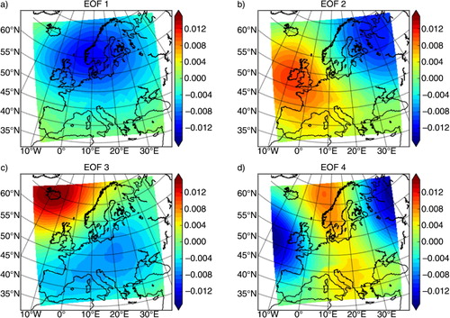
Fig. 3 Thin lines show the mean development of the first four PCs. Thick lines represent the idealised PCs as used for the algorithm. All values are standardised. The day is given relative to the onset of the MBI. Negative days indicate the precursory period whereas positive represent the inflow phase.

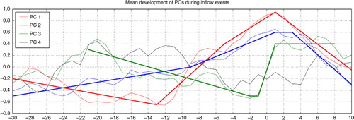
Fig. 4 Correlations between the u-wind component and the mean evolution of PC1 to PC4 as shown in Fig. 3. The correlation is the mean over all 13 training events. The full 41 day periods are used in case of PC1, PC2 and PC4 whereas correlation with PC3 is based only on days considered for the computed correlation threshold of the algorithm – day −21 to day 8. The correlation is based on the mean development of the PCs and not the idealised since there is no idealised PC4.

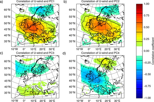
Fig. 5 Same as Fig. 4 but for the v-wind component.

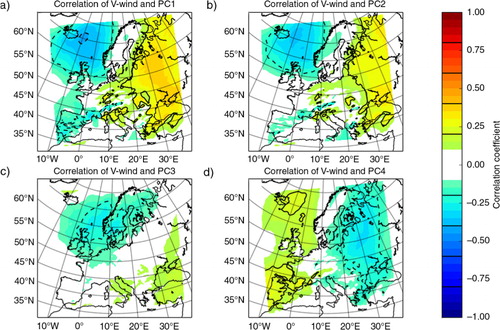
The second EOF pattern (23% explained variance) is a dipole structure with positive values over Great Britain and negative over the White Sea (Fig. 2b). The induced pressure gradients in the area of interest are generally southwest to northeast aligned or vice versa depending on the sign of the corresponding PC. The point correlation maps (Figs. 4 and 5) show that fluctuations in this pattern are linked stronger to changes in the zonal than in the meridional wind. It should be mentioned that both PC1 and PC2 peak in the vicinity of the onset day of the MBI and have at least to some degree a similar overall structure. Hence, it is not surprising that the correlation maps look similar.

Variations of PC3, where the corresponding pattern has an explained variance of 15%, are related to changes of the pressure gradient in the northwest or southeast direction, respectively. The u-wind correlation maps show lower values than for EOF1 and EOF2 but for the v-wind correlations are somewhat higher. Hence, this pattern seems to contribute to changes in the meridional wind. We also consider PC3 for our algorithm because already Matthäus and Schinke (1994) reported a relation between the meridional wind and MBIs.

The fourth EOF pattern (Fig. 2d, 7% explained variance) is a quad-pole with rather weak pressure gradients in the southern Baltic Sea region. However, even the fourth EOF pattern shows some characteristic variability in the vicinity of MBIs. As suggested by the correlation maps, this pattern contributes in the same way as the first two leading modes to fluctuations of the wind components (Figs. 4 and 5). The correlations have, in general, an opposite sign but this is justified by on average opposite PCs (Fig. 3). So, even the fourth pattern contributes with information on fluctuations related to MBIs though with a lower quota than the first two.

The sum of the explained variances for all four considered EOF patterns is 83%. Accordingly, 17% of SLP pattern fluctuations related to MBIs are covered by the remaining EOF patterns of higher order which are not considered during the further investigations.

In the following, we are discussing the development of the PCs averaged over the 13 training events as they depict the intensity and phase of the corresponding EOF. Figure 3 shows the PCs for the first four leading EOFs covering the 30 days of the precursory period through 10 days after the onset of an MBI.

The first PC is negative between day −30 and day −10 with minimum values between days −23 through −11. The negative phase of PC1 can be translated to a high pressure anomaly centred over the southern Scandinavia (Fig. 2a) resembling the composite of Fig. 1. After day −10, PC1 turns positive and peaks around the onset of the MBI. Based on Fig. 4, the mean development of PC1 relates clearly to an increase of the zonal wind component as it is known to be the main driver for MBIs.

PC2 has a distinct positive trend over the entire precursory period. Starting with mean loads of −0.4 at the beginning of the precursory period values become on average positive around day −10. Then, the slope gets stronger until the maximum (+0.6) is reached in the vicinity of the MBI onset. Subsequently, the amplitude of PC2 declines during the inflow period similar to PC1. Similar to PC1 this development can be mainly related to an increase of the westerlies (Figs. 3 and 4). In addition, Fig. 2b shows opposite signs of the EOF pattern over the Baltic Sea and the North Sea. The negative values of PC2 in the preconditioning phase can be translated into higher SLP over the Baltic Sea than over the North Sea. This flips in the vicinity of the onset day according to PC2. The corresponding influence of the SLP changes onto the sea level contributes also positive on the water transfer from the North Sea into the Baltic Sea.

PC3 has a negative slope from day −20 almost until the onset day. Then, the main characteristic of PC3 is a sudden jump in the vicinity of the MBI onset (Fig. 3). While PC3 has its clear minimum just before the onset (days −5 to −1) the maximum is reached directly after the MBI. The rapid transition happens within two days revealing a slope not reached by any other PC.

The mean changes of PC4 are rather small. However, on average MBIs will be more likely if PC4 is positive between days −20 through −10 and negative in the vicinity of the onset day (±5 days).

Changes in the meridional wind related to MBIs show a coherent picture based on the mean development of all PCs (somewhat weaker for PC3) (Fig. 3) and the correlation map (Fig. 5). The meridional wind anomalies are opposite west and east of 10°E, e.g. southerly winds over the North Sea and northerly winds over the Baltic Sea in the early preconditioning phase. Such a wind pattern in combination with weak westerlies or easterlies will clearly help to lower the sea level of the Baltic Sea. During the inflow phase this pattern becomes opposite supporting the inflow event.

3.2. Algorithm

The following section specifies the measures and thresholds used to identify potential MBIs based on SLP variability only. Naturally, these criteria are very much linked to the dynamical development described in Section 3.1.

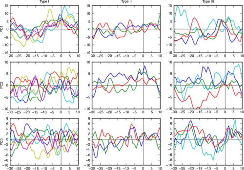
However, checking individual events shows that the mean development is not characteristic for all events in the same manner. Figure 6 shows the development of all training events for the first three modes split into different types. The splitting is based upon the main characteristic in relation to the development of the PCs. For instance, type I events show clearly the increase of PC1 from the middle of the precursory phase towards the onset day. This feature is less developed for type II and type III events (Fig. 6 upper middle and upper right). On the other hand, these types have a better coherence for their corresponding PC as, for example, the steep increase of PC3 in the vicinity of the onset for type III events (Fig. 6 lower right). We distinguish three different types based on the strongest relation to the corresponding PC, for instance type I events have the strongest relation to PC1 and so on.

Fig. 6 Development of the PC1, PC2 and PC3 for all MBIs chosen as training events.

In general, MBIs are identified by strong correlations between the individual PC with the idealised mean development of the training set as shown in Fig. 3. The PC developments were idealised since small daily variations are not supposed to be a feature of the mean development but are rather due to the limited sample size. However, the strength of the correlation is independent of the amplitude which limits the information of correlation coefficients drastically. Consequently, we introduce thresholds of absolute values in addition. Finally, we use the state of the Baltic Sea Index (BSI, Lehmann et al., 2002) to identify MBIs. The BSI is the normalised SLP difference of anomalies between Szczecin and Oslo. Therefore, it includes information inherent already in the first four EOFs. However, the BSI adds information beyond the first four leading modes and uses a different time window which holds additional information, too.

Correlations with the full length of the idealised PC (41 days) are performed for PC1 and PC2 since they show a distinct behaviour over the entire precursory and inflow period (Fig. 3). For PC3, a somewhat shorter period is considered beginning only at day −21 close the average peak of PC3 and ending on day 8. Hereby, the sudden rise in the vicinity to the onset is included as the mean feature of PC3. A correlation with PC4 is omitted for all kind of events since variations are rather small.

As mentioned above, additional criteria are needed since the information of correlations only capture the correct phase with an event. Therefore, we add absolute thresholds based on differences to make sure that the relevant magnitudes are exceeded, which is not captured by correlations. The differences are composed between certain periods, for instance the preconditioning phase and the inflow phase. All threshold values are given in Table 2. In line with the correlation thresholds, the highest requirements are needed for the PC related to the type of event. For instance, type II events have a higher requirement in the absolute value of PC2 (>3.1) than type I (>2) or type III (no requirement) events have for PC2.

Table 2. Threshold values used to identify MBIs

Correlation coefficients (phase)				Absolute differences (amplitudes)
Type	PC1	PC2	PC3	PC1+2	PC1	PC2	PC3	PC4
I	>0.6	>0.18	>0.95	>7	>2 (5)	>1 (any)	>−1.5 (>0)
II	>0.29	>0.5	>2.3 (>5)	>3.1 (>4)	>0.1 (>−0.3)	>−1
III	>0.08 (0.5)	>0.1 (0.5)	>0.64	>2.5 (>6)	>0.65 (>−0.5)

Three different types of events are distinguished and the criteria are shown in the corresponding columns. The left part of the table shows thresholds based on correlations. We use correlation thresholds based on PC1, PC2, PC3, as well as the sum of correlation with PC1 and PC2. The right part of the table shows threshold values based on differences between different periods of the PCs development in time (see text). Red numbers highlight the strongest threshold which, in turn, define the type of event. Values in brackets refer to special cases. Here, green numbers indicate a lower than usual thresholds which in turn requires higher levels for other thresholds (blue).

The periods for the computation of differences vary for the PCs. For PC1 and PC2, we subtract the 10-day minimum of the precursory period from the mean value in the vicinity of the onset day (days −4 to 5). The 10-day minimum is checked in two periods, days −30 to −21 and −20 to −11, since the evolution of events is not identical. Some events reach their minimum in PC1 earlier (green curve in the upper left of Fig. 6) while others reach it later in the preconditioning phase (cyan in the same figure). For PC3, the difference is computed between the 10 days of the inflow period (1–10) and 10 days before the onset (−10 to −1). This difference reflects the mean height of the sudden step happening close to the onset for PC3 (Fig. 3). For PC4 the mean difference between the days −20 to −11 and −5 to +4 is used. This threshold should reflect the on average positive phase of PC4 in the middle of the precursory period compared to the rather low values in the vicinity of the onset day (Fig. 3). All details about the absolute thresholds can be found in Table 2.

Finally, the BSI is used as an additional criteria as mentioned above. There is one BSI threshold for all types. The 20-day average of the BSI in the vicinity of the MBI onset (day −10 to day 10) needs to be lower than 0.1.

In general, each potential MBI is identified with the help of six to eight thresholds including correlation coefficients, absolute values and the BSI (see Table 2). However, each type accepts different values for the same threshold. For instance, the correlation with PC1 needs to be >0.6 for type I events, >0.29 for type II events and >0.08 for type III events. Moreover, some exceptions had to be added due to possible mixtures of types. Whereas most type I events share some coherence with the jump of the PC3, others do not. However, in turn these events show a stronger agreement with PC2. Exceptional values are given in brackets in Table 2 where green (blue) numbers indicate a lower (higher) than usual threshold. So, a type I event can be classified if the following absolute thresholds are fulfilled: PC2 >2, PC3>1 and PC4>−1.5. However, an exception can be made if the threshold for PC3 cannot be fulfilled. Then, higher requirements need to be achieved for PC2 (now>5) and PC4 (now>0).

Due to the dependencies on the type of event and due to the exceptions, the total number of thresholds increases to a total of 27 (Table 2) whereas each individual event is identified by a maximum of eight criteria. Nine thresholds are based on correlations with the idealised PCs whereas 17 limits are based on absolute values. The last threshold is based on the BSI. Finally, depending on the combination of fulfilled thresholds the type of event is defined. Note that out of the 13 training events six are regarded as type I, three as type II and four as type III (Table 3). In general, the differentiation between types of events and the complexity of thresholds accentuate the variability between single events. However, it should be mentioned that single events can fulfil the requirements of more than one type. Consequently, they cannot always be classified exclusively into one class of events.

Table 3. Dates of identified MBIs together with some notes, for example, about corresponding observed events if any

Central date	Notes	Central date	Notes
1961-03-22	Training	1979-04-29
1961-12-02	Training	1979-09-14	Impact on BY5
1962-10-25	16 PSU	1981-06-07
1963-11-18	Training	1982-11-17	Training
1964-02-03	Training	1983-01-13	Training
1964-11-20	Listed MBI	1983-03-07	17.5 PSU
1965-10-30	Training	1986-05-29	2002)
1967-04-25	16 PSU, little on BY5	1991-12-21	Impact on BY5
1967-10-14	1993-01-18	Training
1969-02-01	Training	1993-12-09	17.8 PSU
1969-10-29	Training	1994-03-13	2002)
1970-10-27	Training	1998-02-28	16.5 PSU
1972-03-29	Impact on BY5	1998-10-25	16 PSU
1972-11-11	17 PSU	1999-04-10	16 PSU
1973-11-12	Training	2003-05-10	2006)
1975-12-28	Listed MBI	2003-12-20	18 PSU
1976-04-03	16 PSU, little on BY5	2004-09-22	IOW, little on BY5
1976-11-30	Training	2006-05-26
1977-11-13	Listed MBI	2008-02-29	IOW
1978-09-16	16 PSU	2008-11-22	IOW, BY5
1979-03-10	Impact on BY15	2009-09-30	IOW

Here, Training means that this MBI is part of the events used to train the algorithm. Listed MBI refers to MBIs listed by Matthäus et al. (2008) which were not part of the training events. Other references relate to publications describing barotropic inflows for a corresponding period. IOW corresponds to barotropic inflow events mentioned in the annual report of the Institut of Baltic Research Warnemünde (reports start in 1999, see http://www.io-warnemuende.de/zustand-der-ostsee-2012.html). Salinity declarations refer to high salinity concentrations at BY5 which could have hampered the propagation of saline water into the Baltic Sea (cf. Fig. 7).

To conclude this section, the identification of the training MBI from December 1961 is discussed. The computation of the correlation with the idealised PCs yield the following coefficients for this event 0.76 (PC1), 0.33 (PC2) and 0.42 (PC3) and these values for the computed differences 7.2 (PC1), 3.7 (PC2), 1.3 (PC3) and −0.2 (PC4). Neither the correlation of PC2 as PC3 achieves the required values for type II and type III events, respectively (cf. Table 2). But, the correlations are sufficient to pass the thresholds of the type I. Moreover, all threshold values are achieved to be classified as a type I event. As the BSI fulfils the requirement as well, this event is classified as a type I event.

4. Results

4.1. Validation of the algorithm in the control period

Characteristics of the control period are established by projecting the EOF patterns based on the 13 sample MBIs onto the entire simulation (1961–2010). With the derived PCs running correlation coefficients with the idealised PCs of the training sample (Fig. 3) are computed for the first three PCs as well as the differences of absolute values defined as thresholds (Table 2). After the calculation of the BSI, all values needed by the algorithm to identify MBIs are derived. Hence, we can now automatically detect SLP variability patterns which favour MBIs in the period 1961–2010. In general, we need to keep in mind that the algorithm was trained with and herewith designed to identify MBIs with a strength Q>10 and isolated in time.

An overview over all identified events is given in Table 3. In total, 42 events are identified in the simulated period in which 13 are the re-identified training events. Three events are localised in May, one in June and none in July or August. This implies that the great majority (38 events) is identified in the inflow season (between September and April) which is in agreement with observations (Matthäus and Franck, 1992).

The distribution of identified MBIs in time is illustrated in Fig. 7 in combination with salinity measurements at BY5 and BY15. The majority of events is clearly related to increasing salinity at BY5 and/or BY15. Moreover, the stagnation period between 1983 and 1993 is clearly shown even if there are two potential events identified which are not classified as MBI in observations. However, both potential events identified for May 1986 and December 1991 have a strong effect on the salinity at BY5. The following stagnation period (1993–2003) is also depicted by a strongly reduced number of identified MBIs, e.g. no event between April 1999 and May 2002.

Fig. 7 Near bottom salinities at BY5 (top) and BY15 (bottom). Vertical lines show identified MBIs; black lines are training events whereas red lines represent additional events identified by the algorithm Note that the RCA4 simulation ends in 2010 and consequently later events cannot be identified.

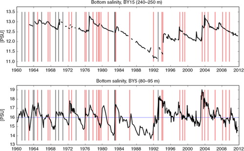
Apart from the training events, three more MBIs listed by Matthäus et al. (2008) are successfully identified. These are the MBIs in November 1964, December 1975/January 1976 and November 1977 (Table 3). Note that the event in November 1977 has only a strength of Q=6 according to Matthäus and Franck (1992). However, the intensity index Q does not always correlate with changes of the salinity condition in the Bornholm and Gotland deeps as stated already by Matthäus and Franck (1992). Examples of classified MBIs without any salinity effect at BY5 or BY15 are the events of 1971 or November 1973, respectively. Meanwhile, the main reason for the interest in MBIs is the fact that they effect the deep Baltic Sea by inflowing highly saline water. As noted for instance by Lehmann et al. (2002) several larger barotropic inflows occurred which did not fulfil the criteria for an MBI. They listed inflow events with more than 150 km³ for the years 1986, 1989, 1990, 1992, 1994, 1995 which were not classified as major inflows by Matthäus et al. (2008). Nevertheless, the three events in May 1986, at the turn of the year 1991/1992 and the one in March 1994 are identified by the algorithm. Especially the former two had significant impact on the salinity at BY5 leading to an increase of more than 1 PSU (Fig. 7). Further identified events which are documented by other sources as barotropic inflows are the events in May 2003 (Matthäus, 2006) as well as the events of the years 2004, 2008 and 2009 (annual reports of the IOW, http://www.io-warnemuende.de/zustand-der-ostsee-2012.html, Table 3).

Other identified events can be clearly related to changes in salinity at BY5 and/or BY15 though they are not documented by any source we are aware of. These events happened in October 1962, April 1967, March 1972, April 1976, March and September 1979 and December 1991. A particular strong increase can be seen at BY5 in March 1972 where the salinity rises from nearly 15 PSU to almost 18 PSU (Fig. 7).

Moreover, a number of events are identified while salinity concentrations were already pretty high. Under such circumstances inflowing water of high salinity could have been blocked (Meier et al., 2006). Consequently, it is possible that despite favourable atmospheric conditions MBIs did not happen. We assume that water masses in the Bornholm Basin with salinities greater than 16 PSU have the potential to block additional inflows (see blue line in Fig. 7). Hence, the identified events in October 1962, April 1967, November 1972, September 1976, March 1983, December 1993, February and October 1998, April 1999 as well as the event at the end of 2003 could have been prohibited by that.

Four identified events remain which are not related to inflows or high salinity as discussed above. These events occurred in October 1967, April 1979, June 1981 and May 2006. Here, the last two events are located outside the observed inflow season and the second happened on the very edge (1979–04–29). Hence, the location within the seasonal cycle could be a contributing factor which prevented these three events. For instance, one reason could be that the maximum climatological river runoff occurs usually in May and higher supply can hamper inflows (Meier and Kauker, 2003).

In summary, 42 atmospheric events with fluctuations favourable for MBIs are identified with the developed algorithm (Table 3); 13 events are consistent with the training dates of observed MBIs. 10 events correspond to barotropic inflows documented in literature (e.g. Lehmann et al., 2002) or in the annual report of the IOW. Furthermore, six events come along with significant peaks in bottom salinity at BY5 and/or BY15. In nine cases, the atmosphere seems favourable for MBIs but, likely, they did not occur due to already high salinity which blocked the event. Three out of 42 cannot be related to observed features nor was there high prevailing salinity with the potential to prevent the event. However, they are identified in the season of climatological maximum river runoff which could have prevented these events. Herewith, only a single identified potential event remains unexplained. Moreover, it should be highlighted that the stagnation periods are clearly recognisable in the time distribution.

4.2. The robustness of the algorithm

The number of training events is small compared to the amount of required criteria. This holds the risk that the criteria are based too strictly on the training events and the algorithm might be tied too strongly to the limited numbers of available targets. This is hard to rule out since we do not have a sufficiently large testing period. A future application of the algorithm to test its robustness could include more inflow events by using e.g. the 20th century reanalysis data (since 1871, Compo et al., 2011) or the recent analogue-based reconstruction of HiResAFF (since 1850, Schenk and Zorita, 2012). However, the quality of reanalysis products or reconstruction decreases further back in time adding new uncertainties. Here, we demonstrate the robustness of the algorithm by presenting the number of identified potential MBIs based on the number of used criteria, e.g. by omitting a certain threshold. The results are summarised in Table 4.

Table 4. The number of identified MBIs based on the number of criteria

Correlations	Absolute values for PC1 & PC2	Absolute values for PC3	Absolute values for PC4	BSI	Identified events
x	x	x	x	x	42
x	x	x	x	–	62 (+20)
x	x	x	–	x	62 (+20)
x	x	x	–	–	85 (+43)
x	x	–	x	x	60 (+18)
x	x	–	x	–	94 (+52)
x	x	–	–	x	79 (+37)
x	–	–	–	x	100 (+58)
x	x	–	–	–	116 (+74)
–	x	x	x	x	152 (+110)
x	–	–	–	–	158 (+116)
–	–	–	–	x	234 (+198)
–	x	x	x	–	278 (+236)

Numbers are given for the hindcast simulation (1961–2010). x indicates that the threshold(s) based on these criteria are used whereas – shows that this criteria is not used. The final column gives the total number of identified events and in brackets the difference to the full algorithm.

Omitting the BSI criteria leads to an additional identification of 20 potential MBIs. The number of events increases by the same number if the absolute threshold for PC4 is omitted. Ignoring both criteria gives 43 additional potential MBIs, which implies that both criteria add almost linearly. The behaviour for PC3 is similar. Omitting PC3 raises the number by 18, omitting PC3 and PC4 adds 37 events to a total of 79. Note that in case of PC3 the absolute value threshold is omitted for type I and type II events only. The threshold is critical for type III and is therefore not left out unless all absolute thresholds are ignored.

The impact of the different kinds of criteria is investigated by using them exclusively (last three lines in Table 4). Using the correlation thresholds only gives 158 potential MBIs. Applying the absolute thresholds leads to 278 identifications whereas the stand-alone BSI finds 234 events. Obviously, the correlation thresholds are the highest burden though being less in number than the absolute thresholds. This implies that the main criterion is the phase captured by the correlations, whereas the magnitudes add as a secondary criterion to the relevant strength in terms of absolute changes of SLP. It should be noted that using the BSI only gives a lot more days fulfilling the criteria. However, since these days are so close to each other they are often counted as a single event. But, whereas using other thresholds the mean number of days fulfilling the criteria is between four and six the number of days is more than 30 when the BSI only is used. However, the BSI criterion in its present form was never intended to identify potential MBIs by itself.

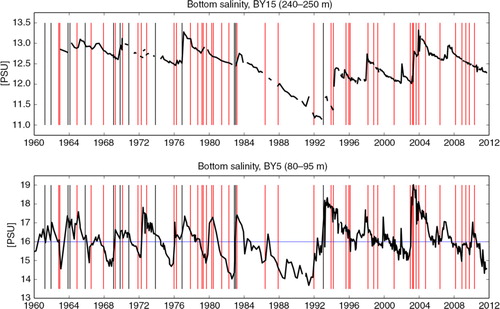
To demonstrate that omitting part of the criteria does not affect the identification of the stagnation periods, we show the time distribution of identified events when the BSI threshold is omitted (Fig. 8). The large majority of additional identified events (+20, see Table 4) are located in inflow active periods enhancing the impression of clustering. For instance, when omitting the BSI threshold three additional events are identified between December 2002 and the end of 2003 summing up to a total of five. On the other hand, very few additional events are identified during the stagnation periods, e.g. one between 1983 and 1993.

Fig. 8 Same as Fig. 7 but for all potential events identified when the BSI criteria is omitted.

It can be concluded that the chosen thresholds are independent from each other to a large degree. Omitting individual thresholds lead to an increase of identifications in a linearly independent way. Moreover, the algorithm turns out to be robust when it comes to the identification of the stagnation periods. This holds true for omitting criteria other than BSI as well (not shown).

4.3. The observed MBI in January 2003

In January 2003 the last strong MBI was observed. In addition, this event is one of the best observed and documented events (e.g. Feistel et al., 2003; Meier et al., 2004; Piechura and Beszczynska-Möller, 2004; Feistel et al., 2006). However, this event is not identified by our algorithm (Table 3) for which reason we investigate it's evolution in more detail.

It is known from observations that the MBI was special in some aspects. For instance, it was accompanied by two smaller events before and two smaller events afterwards (Feistel et al., 2003). Moreover, unlike any previously observed inflow, this one brought very cold water with temperatures around 1–2°C and less into the deep Baltic Sea (Piechura and Beszczynska-Möller, 2004). And, the precursor event in August 2002 was the first ever observed important baroclinic inflow (Feistel et al., 2006). The MBI is classified as a strong MBI with an intensity of Q=20.3 (Matthäus et al., 2008).

The observed onset of the MBI is the 12th of January 2003. Considering this date we show the evolution of the first three PCs over the period relevant for our algorithm (Fig. 9). Obviously, the algorithm fails to identify this event for several reasons. The first PC has a distinct minimum one day before the observed onset which is almost opposite to the mean development of the training events (Fig. 3). Moreover, none of the training events shows such a behaviour independent of the type of event (Fig. 6). However, PC1 has a positive trend during the precursory period which leads overall to a tiny positive correlation with the mean PC1. That is opposite to the mean evolution of PC3 which is almost perfectly anti-correlated with the mean development. Instead of rapidly increasing PC3 decreases strongly in the vicinity of the onset (Fig. 9). Agreement with the training events is restricted to the development of the second PC. Similar to them we see a quite strong increase over the precursory period peaking right after the onset date and decaying thereafter. Consequently, PC2 shows a good correlation of 0.64 with the mean development.

Fig. 9 The evolution of the first three PCs between 2002/12/14 and 2003/01/23. Hence, 2003/01/12 is considered as the onset day which corresponds to the last observed strong MBI.

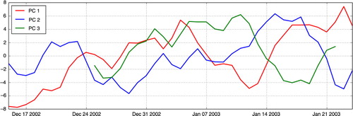
Hence, the event in 2003 is closest to a type II event. However, even matching the high thresholds for PC2 it fails clearly to fulfil the thresholds for PC1 and PC3 of type II events (Table 2). The specific characteristic – at least with respect to our algorithm – is that the SLP-anomaly related to this event is not a negative pressure anomaly over Scandinavia as observed for other MBIs (<−20 hPa, Fig. 1c or Fig. 8B in Matthäus and Schinke (1994)). In contrast to that is the intensification of the pressure gradient based on a strong positive SLP-anomaly over Great Britain (>20 hPa) whereas the pressure over Scandinavia is only slightly reduced (~−7 hPa, not shown). Consequently, the identification of this MBI must fail when our algorithm is applied. This is not satisfying but can be excepted as a minor shortcoming since such events are very rare. The 2003 MBI seems to be the only event characterised by this special feature.

4.4. MBIs in scenario simulations

The algorithm is designed to identify SLP variability necessary for the formation of MBIs. This was done with data from an ERA40 driven simulation with spectral nudging to mimic reality as accurately as possible. However, the derived patterns and hence the algorithm are transferable to any other simulation since they simply refer to SLP conditions necessary for MBIs.

Here, we investigate occurrences of MBIs in a small ensemble of RCA4 simulations forced with three GCMs for the historical period (1961–2005) and scenario simulations considering three different greenhouse gas emission scenarios until the end of the 21st century. The experiments are defined and investigated in more detail by Dieterich et al. (to be submitted to this issue). Note that these GCM driven simulations are run without the spectral nudging technique. Despite the fact that these RCA4 simulations are coupled with the ocean model NEMO-Nordic (see Dieterich et al. to be submitted to this issue) we use SLP fields only to identify MBIs. This illustrates that the algorithm enables us to state something about the potential number of MBIs in climate simulations without explicitly running an ocean model.

Figure 10 shows all identified events and their occurrence in time for all investigated simulations. In addition, total numbers over certain periods are given. First, the number of MBIs is slightly underestimated in the control period when RCA4 is driven with a GCM at the boundary compared to ERA40. In contrast to 38 MBIs identified between 1961 and 2005 in the RCA4-ERA40 simulation (Table 3), we count only 19, 21 and 24 events in the GCM driven simulations (Fig. 10). At least two reasons are plausible for it. First, the small training sample with 13 events only spans a very narrow range of variability making the algorithm not general enough to identify other situations where inflows are generated. Or secondly, the climate generated by the GCMs is simply not favourable for MBIs. For instance, some GCMs are known to have a too strong zonal flow, which in turn could reduce the number of MBIs. A final answer cannot be given taking the limited amount of data into account. However, the 29 events identified in addition to the training events in the control period indicate that the underestimation could be related to the climate produced by the GCMs.

Fig. 10 Identified MBIs in scenario simulations. MPI and EC-Earth continue after the historical period (1961–2005) with the emission scenarios RCP4.5 (top) and RCP8.5 (bottom), respectively. The ECHAM5 simulation is extended with the A1B scenario. Total numbers of identified events are given for the historical and the future (2055–2099) period.

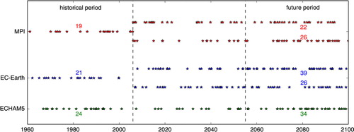
More interesting is the apparent increase in the number of potential MBIs towards the end of this century. As highlighted in Fig. 10 is the potential number of MBIs increasing for all driving GCMs and all scenarios. The increase is small for most scenarios. An outlier is the RCP4.5 realisation of EC-Earth which shows almost a doubling of MBIs. In spite of the considered long periods (45 years each) these results could be affected from long-term variability including the distribution of extensive stagnation periods. Similar to the observed stagnation period 1983–1993, we find several multi-year periods without any identified MBI, e.g. around 2060 in the MPI-RCP8.5 realisation (Fig. 10). Nevertheless, the increase of MBIs in all scenarios provides confidence that atmospheric variability is favourable for more strong inflows in a future climate.

This is underpinned by using the algorithm another time with less thresholds. The slight increase is independent of the used number and combination of thresholds as shown in Table 5. Out of the 30 comparisons between the control (1961–2005) and the future period (2055–2099) we find an increase for the future in 29 cases. The only exception is seen for the MPI-OM simulation when the absolute threshold of PC3 is omitted. However, this does not affect the overall robust yet slight increase.

Table 5. The number of MBIs identified by our algorithm as defined in Section 3.2

Driving GCM	Parameter option	Control period (1961–2005)	RCP4.5 (2055–2099)	RCP8.5/A1B (2055–2099)
MPI-OM	all parameter	19	22	26
MPI-OM	no BSI	25	32	33
MPI-OM	no PC4	23	32	37
MPI-OM	no PC3	33	30	36
MPI-OM	no PC3/4	38	39	46
MPI-OM	no PC3/4, no BSI	59	62	61
EC-Earth	all parameter	21	39	26
EC-Earth	no BSI	28	46	33
EC-Earth	no PC4	27	53	42
EC-Earth	no PC3	29	45	38
EC-Earth	no PC3/4	38	60	52
EC-Earth	no PC3/4, no BSI	55	75	67
ECHAM5	all parameter	24	–	34 (A1B)
ECHAM5	no BSI	34	–	42 (A1B)
ECHAM5	no PC4	33	–	50 (A1B)
ECHAM5	no PC3	38	–	44 (A1B)
ECHAM5	no PC3/4	48	–	60 (A1B)
ECHAM5	no PC3/4, no BSI	64	–	83 (A1B)

Results are shown for RCA4 simulations driven with three different GCMs and three different greenhouse gas emission scenarios, that is, RCP4.5, RCP8.5 and A1B. Total numbers are given for a control period (1961–2005) and the second half of this century (2055–2099). Results are shown using either all or only certain selected criteria.

5. Conclusions and discussion

In this paper, a new method to detect conditions favourable for MBIs has been developed and tested. The algorithm uses daily SLP-fields as the only parameter. A PCA is used to identify the main characteristics of MBIs. Based on the PCA performed with a training sample 27 individual thresholds are defined to identify SLP variability favourable for the development of MBI. However, no potential MBI is identified using more than eight criteria at a time. It is shown that the developed algorithm is capable to identify the majority of MBIs in the control period (1961–2010). Here, a total of 42 events have been identified. Thereof, 13 events are the training events, 16 are successfully identified events, in nine cases the atmospheric requirements are fulfilled but the event did not occur due to too high salinity concentrations blocking the inflowing water and three events are likely prevented by strong river runoff. The hampering effect of stronger freshwater supply by river runoff and net precipitation is known from literature (e.g. Schinke and Matthäus, 1998; Matthäus and Schinke, 1999; Meier and Kauker, 2003) but not investigated for the events identified by our algorithm. That is also the case for events likely blocked by salty water as documented by Meier et al. (2006). Corresponding investigations are omitted in this manuscript because the focus of it is purely on atmospheric requirements without any restrictions from the ocean.

The algorithm considers a precursory period of 30 days, the onset day and 10 days thereafter and according to these 41 days in total. This period is rather short when compared with other studies which investigated atmospheric requirements for MBIs. For instance, positive SLP anomalies over the Baltic already from late summer to autumn are documented by Schinke and Matthäus (1998). It is also documented that stronger westerly winds in autumn are not favourable for MBIs because the Baltic Sea is then already filled up and inflows are hardly possible afterwards (Gräwe et al., 2013). Accordingly, Lass and Matthäus (1996) showed that the mean sea level of the Baltic in October is different between both ensemble means (with and without MBI) with a likelihood of more than 99%. However, our results suggest that – from an atmospheric point of view – SLP variability with a time frame of 41 days is sufficient to generate MBIs as long as other factors (salinity and freshwater supply) do not preclude it.

As mentioned above, identified events can be prohibited by other factors not considered in the algorithm, e.g. river discharge. However, without SLP variability favourable for MBIs no inflow will happen independently from any other parameter. Hence, turning the algorithm around, the algorithm inherits also the capability to identify atmospheric variability not favourable for MBIs. A lack of identified MBIs clearly matches the stagnation period 1983–1993, which is outstanding in the control period. This is a clear success of the algorithm. Moreover, based on this result it can be concluded that the stagnation period is mainly a consequence of missing the particular atmospheric variability needed for MBIs. That is in line with wind analysis done by Lass and Matthäus (1996). They stated that the probability of both negative north and negative east components of the wind with duration of more than 10 days was slightly larger during the period of regular inflow events than during the period of reduced inflow from 1976 to 1992. Increased runoff or freshwater supply in general as mentioned in earlier studies (Schinke and Matthäus, 1998; Meier and Kauker, 2003) seems to be only of secondary importance for the stagnation period but could have contributed as well.

The only severe MBI which is clearly missing is the MBI in January 2003. However, as known from literature this event was very special from many perspectives (e.g. Feistel et al., 2003; Piechura and Beszczynska-Möller, 2004; Feistel et al., 2006). Here, we demonstrated that the evolution of the SLP-pattern related to the event is not comparable with any other MBI which makes it impossible to detect this event with the developed algorithm.

Finally, we applied the algorithm to a small ensemble of scenario simulations. Based on these results, we conclude that atmospheric variability favourable for MBIs intensifies in future climate. However, so far no study reported similar results but studies highlight the reduction of salinity in the Baltic Sea as one of the significant features of climate change (e.g. Meier et al., 2012). Gräwe et al. (2013) find a reduction of MBIs in their scenario simulations. Conversely, they find extreme events towards the end of their scenarios which outmatch any MBI of the control period. Anyway, our results reflect changes in atmospheric requirements for strong MBIs only whereas other results are mainly based on ocean simulations. In that sense, we agree with conclusions by Gräwe et al. (2013) who stated that the necessary preconditioning of the atmosphere is still given in the future with the difference that our findings show an improvement of atmospheric requirements. The broad agreement on salinity reduction in the Baltic Sea will be driven by increased freshwater supply as noted in many studies (e.g. Meier et al., 2012; Gräwe et al., 2013) and is therefore not in contrast with our findings.

The results presented in this paper open up the possibility for several following studies. For instance, our understanding of long-term variations of inflow events could be improved by going further back in time using the algorithm for the 20th century reanalysis data (since 1871, Compo et al., 2011) or the recent analogue-based reconstruction of HiResAFF (since 1850, Schenk and Zorita, 2012). Or, using an ocean model or a coupled atmosphere–ocean model it could be investigated in how far the three types of events can be related to different responses of the ocean. It is known that the relation of water entering the Baltic Sea through the Great Belt or the Öresund varies significantly between different events (Fischer and Matthäus, 1996). Here, it could be tested if these differences can be related to the three types. Moreover, it should be investigated if the future increase in atmospheric variability favourable for MBIs can be related to any large scale features as the NAO or blocking frequencies/characteristics over the North Atlantic Ocean.

If required, we are happy to provide the source code of the algorithm (a Python program) to any interested reader.

6. Acknowledgements

The research presented in this study is part of the Baltic Earth programme (Earth System Science for the Baltic Sea region, see http://www.baltex-research.eu/balticearth) and was funded by the Swedish Research Council for Environment, Agricultural Sciences and Spatial Planning (FORMAS) within the projects ‘Impact of accelerated future global mean sea level rise on the phosphorus cycle in the Baltic Sea’ (Grant no. 214-2009-577) and ‘Impact of changing climate on circulation and biogeochemical cycles of the integrated North Sea and Baltic Sea system’ (Grant no. 214-2010-1575) and from Stockholm University's Strategic Marine Environmental Research Funds ‘Baltic Ecosystem Adaptive Management’ (BEAM). Additional support came from the Norden Top-level Research Initiative sub-programme ‘Effect Studies and Adaptation to Climate Change’ through the ‘Nordic Centre for Research on Marine Ecosystems and Resources under Climate Change’ (NorMER). The scenario simulations used in this study have been funded by the ‘Impacts of Climate Change on Waterways and Navigation’ KLIWAS program. KLIWAS is a joint research program of the German Federal Institute of Hydrology (BfG), the German Federal Waterways and Engineering and Research Institute (BAW), the National Weather Service of Germany (DWD) and the Federal Maritime and Hydrographic Agency (BSH) in co-operation with universities and other research institutions. KLIWAS is funded by the Federal Ministry of Transport, Building and Urban Development (BMVBS). The simulations have been conducted on the Linux clusters Krypton and Triolith, both operated by the National Supercomputer Centre in Sweden (NSC). Resources on Triolith have been made available by the Grant SNIC 002/12-25 ‘Regional climate modelling for the North Sea and Baltic Sea regions’ provided by the Swedish National infrastructure for Computing (SNIC). Salinity data used in this paper are collected from the SMHI data base SHARK (Svenskt HavsARKiv, see http://www.smhi.se/oceanografi/oce_info_data/SODC/overview.htm). Data have been collected within the coordinated Swedish environmental monitoring program by SMHI, UMF and SMF.

References

- Berg P. , Doscher R. , Koenigk T . Impacts of using spectral nudging on regional climate model RCA4 simulations of the Arctic. Geosci. Model Dev. 2013; 6: 849–859.
- Compo G. P. , Whitaker J. S. , Sardeshmukh P. D. , Matsui N. , Allan R. J. , co-authors . The Twentieth Century Reanalysis Project. Q. J. Roy. Meteor. Soc. 2011; 137: 1–28. Online at: http://dx.doi.org/10.1002/qj.776 .
- Feistel R. , Nausch G. , Hagen E . Unusual Baltic inflow activity in 2002–2003 and varying deep-water properties. Oceanol. 2006; 21–35. Online at: http://www.iopan.gda.pl/oceanologia/48Sfeist.pdf, 5th Baltic Sea Science Congress, Sopot, Poland, Jun 20–24, 2005.
- Feistel R. , Nausch G. , Matthaus W. , Hagen E . Temporal and spatial evolution of the Baltic deep water renewal in spring 2003. Oceanol. 2003; 623–642. 3rd Baltic Sea Science Congress, Helsinki, Finland, Aug, 2003.
- Fischer H. , Matthäus W . The importance of the Drogden Sill in the Sound for major Baltic inflows. J. Marine Syst. 1996; 9: 137–157.
- Gräwe U. , Friedland R. , Burchard H . The future of the western Baltic Sea: two possible scenarios. Ocean Dynam. 2013; 63: 901–921. Online at: http://dx.doi.org/10.1007/s10236-013-0634-0 .
- Gustafsson B. G. , Andersson H. C . Modelling the exchange of the Baltic Sea from the meridional atmospheric pressure difference across the North Sea. J. Geophys. Res. 2001; 106: 19731–19744.
- Hordoir R. , Dieterich C. , Basu C. , Dietze H. , Meier H. E. M . Freshwater outflow of the Baltic Sea and transport in the Norwegian current: A statistical correlation analysis based on a numerical experiment. Continental Shelf Research. 2013; 106: 1–9. DOI: 10.1016/j.crs.2013.05.006.
- Hordoir R. , Meier H. E. M . Freshwater fluxes in the Baltic Sea: a model study. J. Geophys. Res. 115: 028.
- Lass H. U. , Matthäus W . On temporal wind variations forcing salt water inflows into the Baltic Sea. Tellus A. 1996; 48: 663–671. http://dx.doi.org/10.1034/j.1600-0870.1996.t01-4-00005.x .
- Lehmann A. , Krauss W. , Hinrichsen H . Effects of remote and local atmospheric forcing on circulation and upwelling in the Baltic Sea. Tellus A Dyn. Meteorol. Oceanogr. 2002; 54: 299–316.
- Matthäus W . The history of investigations of salt water inflows into the Baltic Sea – from the early beginning to recent results. 2006. Meereswissenschaftliche Berichte 65, Institut für Ostseeforschung Warnemünde, Rostock, Germany.
- Matthäus W. , Franck H . Characteristics of major Baltic inflows – a statistical analysis. Cont. Shelf Res. 1992; 1375–1400. Online at: http://www.sciencedirect.com/science/article/pii/027843439290060W .
- Matthäus W. , Nehring D. , Feistel R. , Nausch G. , Mohrholz V. , co-authors . The inflow of highly saline water into the Baltic Sea. 2008; Hoboken, NJ, USA: John Wiley & Sons, Inc.. 265–309. Online at: http://dx.doi.org/10.1002/9780470283134.ch10 .
- Matthäus W. , Schinke H . Mean atmospheric circulation patterns associated with major Baltic inflows. Deutsche Hydrografische Zeitschrift. 46: 321–339. Online at: http://dx.doi.org/10.1007/BF02226309 .
- Matthäus W. , Schinke H . The influence of river runoff on deep water conditions of the Baltic Sea. Hydrobiol. 1999; 393: 1–10. Joint BMB 15 / ECSA 27 Symposium, Aland, Finland, Jun, 1997.
- Meier H. , Doscher R. , Broman B. , Piechura J . The major Baltic inflow in January 2003 and preconditioning by smaller inflows in summer/autumn 2002: a model study. Oceanol. 2004; 46: 557–579.
- Meier H. E. M. , Andersson H. C. , Arheimer B. , Blenckner T. , Chubarenko B. , co-authors . Comparing reconstructed past variations and future projections of the Baltic Sea ecosystem – first results from multi-model ensemble simulations. Environ. Res. Lett. 2012; 7: 034005. Online at: http://stacks.iop.org/1748-9326/7/i=3/a=034005 .
- Meier H. E. M. , Feistel R. , Piechura J. , Arneborg L. , Burchard H. , co-authors . Ventilation of the Baltic Sea deep water: a brief review of present knowledge from observations and models. Oceanol. 2006; 48: 133–164. 5th Baltic Sea Science Congress, Sopot, Poland, Jun 20–24, 2005.
- Meier H. E. M. , Kauker F . Modeling decadal variability of the Baltic Sea: 2. Role of freshwater inflow and large-scale atmospheric circulation for salinity. J. Geophys. Res. 2003; 108: 3368.
- Mironov D. , Heise E. , Kourzeneva E. , Ritter B. , Schneider N. , co-authors . Implementation of the lake parameterisation scheme FLake into the numerical weather prediction model COSMO. Boreal Env. Res. 2010; 15: 218–230.
- Piechura J. , Beszczynska-Möller A . Inflow waters in the deep regions of the southern Baltic Sea – transport and transformations (vol 45, pg 593, 2003). Oceanol. 2004; 46: 113–141. Online at: http://www.iopan.gda.pl/oceanologia/46_1.html .
- Samuelsson P. , Jones C. G. , Willen U. , Ullerstig A. , Gollvik S. , co-authors . The Rossby Centre Regional Climate model RCA3: model description and performance. Tellus A. 2011; 63: 4–23.
- Schenk F. , Zorita E . Reconstruction of high resolution atmospheric fields for Northern Europe using analog-upscaling. Clim. Past Discuss. 2012; 8: 819–868. Online at: http://www.clim-past-discuss.net/8/819/2012 .
- Schinke H. , Matthäus W . On the causes of major Baltic inflows – an analysis of long time series. Cont. Shelf Res. 1998; 18: 67–97. Online at: http://www.sciencedirect.com/science/article/pii/S027843439700071X .
- Unden P. , Rontu L. , Järvinen H. , Lynch P. , Calvo J. , co-authors . HIRLAM-5 scientific documentation. 2002. Technical Report, Swedish Meteorological and Hydrological Institute (SMHI), Sweden, Norrkping.
- Uppala S. M. , Kallberg P. W. , Simmons A. J. , Andrae U. , Bechtold V. D. C. , others . The ERA-40 re-analysis. Q. J. Roy. Meteorol. Soc. 2005; 131: 2961–3012.
- Wang S. , Dieterich C. , Döscher R. , Höglund A. , Hordoir R. , Meier H. E. M. , co-authors . Development and evaluation of a new regional coupled atmosphere-ocean model RCA4-NEMO and application for future scenario experiments. Tellus. 2013
- Zorita E. , Laine A . Dependence of salinity and oxygen concentrations in the Baltic Sea on large-scale atmospheric circulation. Clim. Res. 2000; 14: 25–41.