Stochastically driven transitions between climate attractors

Abstract

The classical non-linear climatic model previously developed by Saltzman with co-authors and Nicolis is analysed in both the deterministic and stochastic cases in a wider domain of system parameters. A detailed analysis of the deterministic model shows a co-existence of a stable cycle and equilibrium phase points of the climate system localisation. A fine structure of attraction basins existing around stable equilibria is studied. The model under consideration possesses the noise-induced transitions between possible system attractors (limit cycle and two equilibria) in the case of stochastic dynamics caused by temperature fluctuations. A new phenomenon of stochastic generation of large amplitude oscillations around two equilibrium points in the absence of a limit cycle is revealed. The co-existence of large-, small- and mixed-mode stochastic transitions between the climate system attractors is found.

• climatic model
• stochastic disturbances
• noise-induced transitions
• attraction basins

1. Introduction

The interaction between non-linearity and stochasticity in dynamical systems can generate unexpected phenomena, which have no analogue in the deterministic case. New stochastic regimes such as noise-induced transitions (Horsthemke and Lefever, 1984; Anishchenko et al., 2007), stochastic bifurcations (Arnold, 1998), stochastic resonance (Gammaitoni et al., 1998; McDonnell et al., 2008), noise-induced chaos (Lai and Tél, 2011) and noise-induced excitability (Lindner et al., 2004) attract attention of researchers in mechanics, biophysics and geophysics. Stochastic effects in non-linear models are the subjects of intensive investigations in climate dynamics (Imkeller and Von Storch, 2001; Saltzman, 2002; Chekroun et al., 2011).

It is well-known that the Earth's climatic system possesses potential possibilities for external and internal feedbacks of both positive and negative signs (e.g. Earth orbital radiation and anthropogenic CO₂ changes, changes in the atmospheric composition and temperature due to unpredictable volcanic eruptions, the natural variability of system variables due to uncertainties in their initial conditions and due to the presence of stochastic noises). This complex behaviour is responsible for the oscillatory, damping or amplifying climate dynamics on many time scales (Saltzman and Moritz, 1980; Saltzman et al., 1981; Selvam, 2007; Crucifix, 2012). It should be mentioned that the quasi-periodic and irregular climatic variations dependent of these feedbacks have been revealed in a number of geological records (Alley et al., 2003; Thurow et al., 2009; White et al., 2010; Holmes et al., 2011). It was shown previously that the climatic system fluctuations near an unstable equilibrium are connected with a dominant positive feedback in a certain domain of physical parameters (Saltzman et al., 1981). If this is really the case, the system can never settle down, but is prevented from running away catastrophically by powerful negative feedbacks that dominate when the departures from equilibrium become great.

Another scenario of climate dynamics can be demonstrated on the basis of a simple model of sea ice–ocean temperature oscillator, in which the destabilising CO₂ temperature and ice-baroclinicity feedbacks are absent. In this case, the climatic system fluctuates in the vicinity of a stable equilibrium associated with dominant negative feedback (Saltzman, 1978, 1982). The possibility of complex, non-periodic behaviour and, in particular, the existence of a chaotic attractor as well as of long period solutions on the basis of a simple Saltzman type model has been demonstrated previously by Nicolis (1987).

This paper is concerned with a more detailed study of this model in the case of its deterministic and stochastic dynamics for a wider domain of system parameters with new qualitatively different regimes. For this climatic model, the existence of noise-induced transitions between a limit cycle and equilibrium phase points, as well as a phenomenon of stochastic generation of large-amplitude oscillations, are demonstrated for the first time. For the analysis of noise-induced phenomena, a stochastic sensitivity function technique is used (Bashkirtseva and Ryashko, 2004, 2011). Mathematical background of this technique is presented in Appendix.

2. Deterministic model

Let us consider the dynamical system of the following coupled autonomous equations governing the departures of the sine of the marine-ice latitude (η′) and the average temperature of the entire ocean (θ′) from their equilibrium values (Saltzman, 1978; Saltzman et al., 1981)1 where , , is the time, the primes denote departures from an equilibrium (η′=0, θ′=0); φ ₁, φ ₂, , and are positive constants. The coefficients φ ₁ and φ ₂, respectively, are proportional to the upward flux of heat from the ocean at the ice edge and the fully transmitted radiation absorbed at the surface (Saltzman, 1978). In addition, the latent heat of fusion and the ice mass inertia factor appear in the denominators of φ ₁ and φ ₂. This factor reflects the fact that the marine ice represents a combination of ‘pack’ and ‘shelf’ forms (Saltzman et al., 1982). The coefficient is responsible for the sensible and latent heat fluxes along with the non-CO₂ effects of longwave radiative fluxes (Saltzman et al., 1981). The departure of the atmospheric CO₂ concentration from its equilibrium value is described by the coefficient whereas the non-linear contribution to the vertical heat flux at the surface is characterised by the term with (Saltzman et al., 1981).

Introducing the following variables and parameters2 we rewrite the dynamical system (1) in dimensionless form3

Here a and b are positive parameters [their physical meaning is given by coefficients φ ₁, φ ₂, and in accordance with eq. (2)], t is the dimensionless time, and the modified variables x and y describe the sine of the multi-annual mean sea ice latitude and the bulk ocean temperature, respectively. The linear terms in the right-hand side characterise a damped harmonic oscillation due to the ‘ice-insulator’ effect described by Saltzman (1978) and a linear destabilising effect caused by a positive feedback between atmospheric CO₂ concentration and mean temperature of the ocean (Saltzman and Moritz, 1980). A non-linear restorative mechanism that is dominant when the climatic system is far from its equilibrium is described by the non-linear term x ² y (Saltzman et al., 1981). Note that a=6.4 and b=4 in the original model studied by Saltzman et al. (1981).

For any a and b, the system (3) has a trivial equilibrium M ₀(0,0). This equilibrium is stable for b<1 and b<a (zone D in Fig. 1).

Fig. 1 Zones of equilibria.

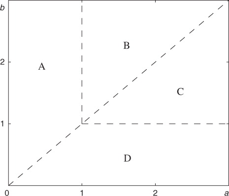
For b>a, this system has a pair of non-trivial symmetric equilibria and (zone A⋃B). Here . These equilibria are stable for a<1 and b>a (zone A in Fig. 1).

Dynamics of the system (3) in zone D is trivial: all trajectories are attracted to the stable equilibrium M ₀. The border between zones C and D (a>1, b=1) is a line of the Andronov–Hopf bifurcation. When passing through this border from D to C, the equilibrium M ₀ loses a stability and a stable limit cycle is born. Note that Saltzman studied a dynamics of this model in zone C where all trajectories are attracted to the stable limit cycle.

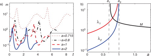
Here we consider in detail a dynamics of the system (3) in zones A, B and C. We fix the parameter b=2 and vary the parameter a. In Fig. 2, y-coordinates of the attractors and repellers of the system (3) are shown. Here, thin solid lines plot stable equilibria, dashed lines show unstable equilibria, thick solid lines present extrema of stable cycles, and dash-dotted lines illustrate extrema of unstable cycles. For the parameter a, one can mark four bifurcation values: a ₁≈0.714, a ₂≈0.775, a ₃=1 and a ₄=2. Note that a ₁ and a ₂ were found numerically.

Fig. 2 Bifurcation diagram: y-coordinates of stable equilibria (thin solid lines), unstable equilibria (dashed lines), extrema of stable cycles (thick solid lines) and extrema of unstable cycles (dash-dotted lines).

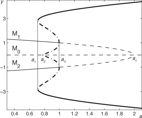
For a>a ₄, the deterministic system (3) exhibits a stable limit cycle, which embraces the unique unstable equilibrium M ₀. For a ₃<a<a ₄, along with the stable cycle, this system has three unstable equilibria M ₀, M ₁ and M ₂. As the parameter a passes a ₃, the equilibria M ₁ and M ₂ become stable and two separate unstable cycles appear around them. As the reducing parameter a passes a ₂, these unstable cycles are merged into one. At the point a=a ₁ this big unstable cycle merges with stable one and for a<a ₁ the system (3) exhibits two stable equilibria M ₁, M ₂ separated by the unstable equilibrium M ₀. Note that for a<a ₄, the equilibrium M ₀ is the saddle point, and for a>a ₄, M ₀ is the unstable node.

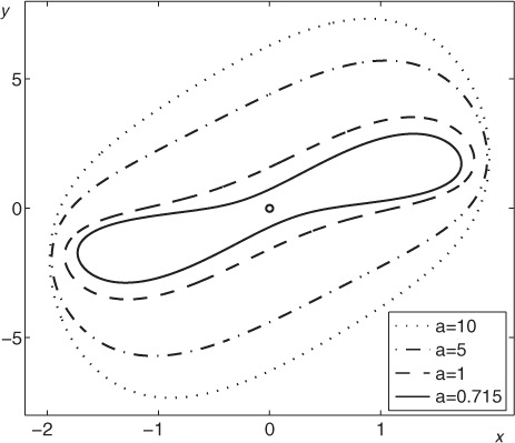
In Fig. 3, stable cycles of the system (3) are plotted for a>a ₁. It is worth noting that x-amplitude changes insignificantly while y-amplitude grows with a.

Fig. 3 Cycles of the deterministic system for b=2.

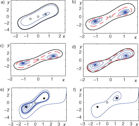
In Fig. 4, a set of typical phase portraits is presented for various values of the parameter a. Here, thick solid black lines plot stable cycles, unstable cycles are plotted by dashed red lines, stable (unstable) equilibria are shown by filled (empty) circles, and thin blue solid lines plot phase trajectories. Here, unstable cycles play a role of separatrices between basins of attraction of stable equilibria and a limit cycle.

Fig. 4 Phase portraits of the deterministic system with b=2 for (a) a=1.5, (b) a=0.8, (c) a=0.76, (d) a=0.715, (e) a=0.7, (f) a=0.5 Stable cycles (thick solid black lines), unstable cycles (dashed red lines), stable equilibria (filled circles), unstable equilibria (empty circles) and phase trajectories (thin blue solid lines).

3. Stochastic model

Consider a stochastic system4 Here w is a standard Wiener process and ɛ is an intensity of random disturbances. This stochastic model reflects an influence of random fluctuations of the mean ocean temperature.

For a numerical simulation of random trajectories of this stochastic system, the Euler-Maruyama scheme (Kloeden and Platen, 1992) with the time step Δt=10⁻⁴ was used. To exclude the possibility that these results are just some peculiar effect of the particular step size, the calculations were repeated with other step sizes to ensure that the same dynamical behaviour is obtained. For the modelling of appropriate stochastic components of normally distributed random disturbances in the Euler-Maruyama scheme, the standard Box-Muller transform (Box and Muller, 1958) was used.

Under the stochastic disturbances, random trajectories leave deterministic attractors and form probabilistic distribution around it. These stable stationary probabilistic distributions describe corresponding stochastic attractors. For weak noise, random states of stochastic attractors are concentrated nearby deterministic attractors. Random states of the system (4) with ɛ=0.01 are plotted by grey points around the stable equilibrium M ₁ for a=0.7 (Fig. 5a),and around the stable limit cycle for a=1.1 (Fig. 5b). Here, random states are points of the random trajectory calculated numerically after a sufficiently long transient time (T=10⁵). These states adequately reflect a corresponding stationary probability density.

Fig. 5 Random states (grey) of stochastic attractors and confidence domains (dashed lines): (a) confidence ellipse around the equilibrium M ₂ for a=0.5, ɛ=0.01; (b) confidence band around the limit cycle for a=1.1, ɛ=0.05.

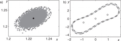
A dispersion of random states in stochastic attractors depends on the stochastic sensitivity of initial deterministic attractors (see Appendix). Stochastic sensitivity functions technique allows us to construct confidence domains where random states are arranged with the assigned fiducial probability. In Fig. 5, the confidence ellipse and confidence band with fiducial probability P=0.99 are plotted by dashed lines. As one can see, these confidence domains give a good description of the spatial arrangement of random states in stochastic attractors.

The stochastic sensitivity of the equilibria M _1,2 is defined by the eigenvalues of the matrix W. For the description of the stochastic sensitivity of the limit cycle, the function m(t) and the stochastic sensitivity factor M=max m(t), t∈[0, T] are used (see Appendix). In Fig. 6a, plots of the function m(t) are shown for different values of a. As one can see, the stochastic sensitivity along the cycle is non-uniform. Moreover, a quantity of the peaks of the function m(t) changes with the parameter a variation. Graphs and M as functions of the parameter a are presented in Fig. 6b. Note that the stochastic sensitivity depends essentially on the parameter a and rises unlimitedly near bifurcation points a ₁ and a ₃. Compare the stochastic sensitivity of stable cycles and stable equilibria M _1,2 on the interval (a ₁, a ₃) where they coexist. Near a ₁, the cycle is more sensitive than equilibria, and near a ₃ vice versa. Note that this difference in the sensitivity defines the direction of noise-induced transitions between cycle and equilibria.

Fig. 6 Stochastic sensitivity of attractors: (a) plots m(t) for cycles; (b) plots for equilibria and M(a) for cycles.

As the noise intensity increases, random trajectories can cross separatrices between basins of attraction and exhibit new dynamical regimes, which have no analogue in the deterministic case. Scenarios of such noise-induced transitions depend on the peculiarities of the mutual arrangement of deterministic attractors and repellers on the phase plain.

First consider the interval a ₁<a<a ₃. Here, the deterministic system (3) has a stable cycle and two stable equilibria M ₁, M ₂ as attractors, and unstable cycles and unstable equilibrium M ₀ as repellers. In Fig. 7, qualitative changes in stochastic dynamics of the system (4) for a=0.76 are shown for three values of ɛ. Here, random trajectories starting from equilibria M ₁, M ₂ are plotted by black colour, and trajectories starting from a cycle are plotted by grey colour. For weak noise (ɛ=0.05), random trajectories are concentrated nearby initial deterministic attractors (see Fig. 7a). Here, random trajectories starting from the equilibria demonstrate small-amplitude stochastic oscillations (SASO), and random trajectories starting from the cycle execute large-amplitude stochastic oscillations (LASO).

Fig. 7 Stochastic trajectories for a=0.76 and (a) ɛ=0.05; (b) ɛ=0.1; (c) ɛ=0.2.

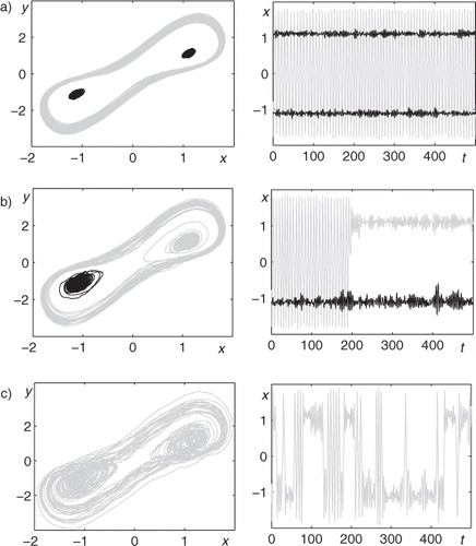
As noise intensity increases (ɛ=0.1), random trajectories starting from the equilibrium are localised nearby this initial point, but a trajectory starting from the cycle, after several turns along it passes into the vicinity of the equilibrium (see Fig. 7b). Here the system (4) exhibits a transition ‘cycle → equilibrium’. So, independently on initial state, the stochastic system transits to SASO regime. With further increase of noise the reverse transitions ‘equilibrium → cycle’ begin. In Fig. 7c (ɛ=0.2) noise-induced transitions between basins of attraction of equilibria M ₁, M ₂ and the cycle are observed with a high probability. Thus, when noise exceeds some threshold the stochastic system demonstrates mixed-mode stochastic oscillations (MMSO) with the intermittency of SASO and LASO.

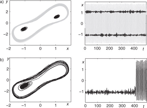
Consider now a=0.82. For weak noise (ɛ=0.05), random trajectories are also concentrated nearby initial deterministic attractors separately (see Fig. 8a). As noise intensity increases (ɛ=0.1), at first, noise-induced transitions ‘equilibrium → cycle’ appear (see Fig. 8b). Note that random trajectories starting from the cycle are localised nearby this close curve. Here, independently on initial state, the stochastic system transits to LASO regime. With further increase of noise, the transitions ‘cycle → equilibrium’ also begin and the system exhibits MMSO.

Fig. 8 Stochastic trajectories for a=0.82 and (a) ɛ=0.05; (b) ɛ=0.1.

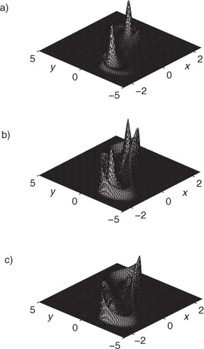
So, in the interval a ₁<a<a ₃, where the deterministic system exhibits three isolated attractors, due to stochastic mixing, a combined trimodal stochastic attractor is observed. In Fig. 9, for a=0.76, a=0.82, a=0.86 the plots of the probability density function of stochastic attractors are presented for the same noise ɛ=0.2. Here, one can see a closed ridge which embraces two peaks. These peaks are located above the stable equilibria, and the ridge lies above the curve of the deterministic cycle. For a=0.76, peaks dominate (see Fig. 9a). This means that phase trajectories of the stochastic system spend most of their time in a small region around the equilibria. For a=0.86, the dominant of the attractor is a ridge because the random trajectories are more often located in the basin of attraction of the limit cycle.

Fig. 9 Probability density function for ɛ=0.2 and (a) a=0.76; (b) a=0.82; (c) a=0.86.

Consider now the interval 0<a<a ₁ where the deterministic system (3) has two stable equilibria M ₁, M ₂ only. Fix a=0.7. For weak noise (ɛ=0.1), random trajectories starting from the equilibria are located nearby initial points (see Fig. 10a). As noise intensity increases (ɛ=0.2), random trajectories begin to transit between neighbourhoods of M ₁ and M ₂ (see Fig. 10b). 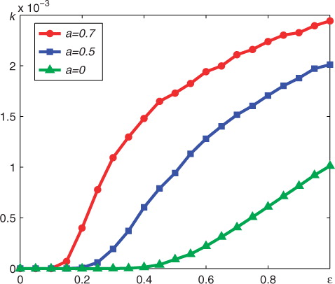Note that transient between M ₁ and M ₂ includes some turns around both equilibria. It looks like a movement along some closed curve similar to limit cycle. Here, a transition scenario is as follows: SASO around the equilibrium – LASO around both equilibria – SASO around the equilibrium and so on. With further increase of noise, a percentage of LASO increases (see Fig. 10c for ɛ=0.3). The percentage of these LASO in a common mixed-mode process x(t) on the interval [0, T] can be estimated by the value where n is a quantity of intersections of x(t) with x=0. A dependence of the value k on the parameters a and ɛ is presented in Fig. 11. It can be seen that this function increases non-uniformly with zones of the slow and fast growth. The beginning of the fast growth allows us to estimate the threshold noise intensity corresponding to the transition from the SASO to MMSO regime. This threshold value depends on the stochastic sensitivity of the equilibrium. Note that the higher the sensitivity of the equilibrium, the lower the threshold value (compare Figs. 6b and 11).

Fig. 10 Stochastic trajectories for a=0.7 and (a) ɛ=0.1; (b) ɛ=0.2; (c) ɛ=0.3.

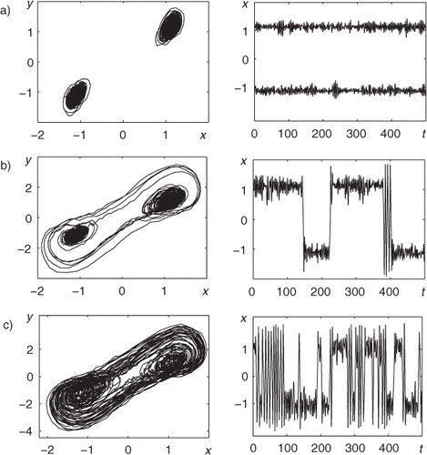
Fig. 11 Plot of k(ɛ).

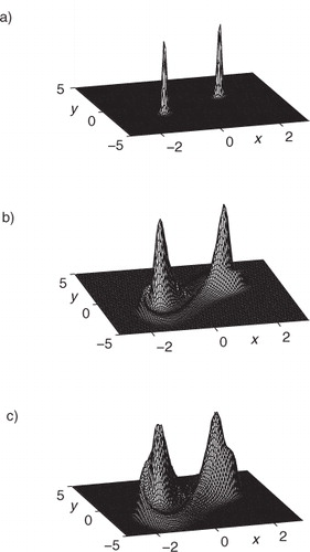
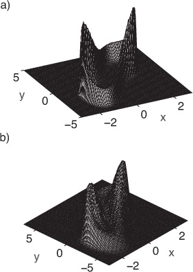
In Fig. 12, for a=0.7 and ɛ=0.1, 0.3, 0.5 plots of the probability density function of stochastic attractors are presented. Here, along with two anticipated peaks corresponding to the stable equilibria, one can see an unexpected closed ridge connecting peaks (see Fig. 12b and 12c). In this case, such a ridge does not have a deterministic cycle as an underlying reason. A key for understanding this phenomenon is a non-uniformity of the phase portrait of the initial deterministic system. Indeed, in Fig. 4e, it is clearly seen that deterministic trajectory going to the equilibrium passes a zone of so-called ‘transient attractor’ with temporary local stabilisation. With an increase of noise a percentage of LASO increases too, and this ridge becomes higher. Thus, it can be interpreted as noise-induced generation of the transient stochastic cycle in a zone where the deterministic system has stable equilibria only.

Fig. 12 Probability density function for a=0.7 and (a) ɛ=0.1; (b) ɛ=0.3; (c) ɛ=0.5.

Consider the interval a ₃<a<2 where the deterministic system (3) has a stable limit cycle as a single attractor. For weak noise (see Fig. 13a for a=1.1, ɛ=0.2), random trajectories with LASO are concentrated nearby initial deterministic cycle. For increasing noise, small-amplitude scrolls appear near unstable equilibria (see Fig. 13b for a=1.1, ɛ=1). A percentage of LASO in a common MMSO regime is reduced slightly (see Fig. 14). In Fig. 15, plots of the probability density function of stochastic attractors are shown. Here, two peaks are parts of the closed ridge. A noise-induced generation of the small-amplitude stochastic scrolls increases the relative thickness of the inner slopes of these peaks.

Fig. 13 Stochastic trajectories for a=1.1 and (a) ɛ=0.2; (b) ɛ=1.

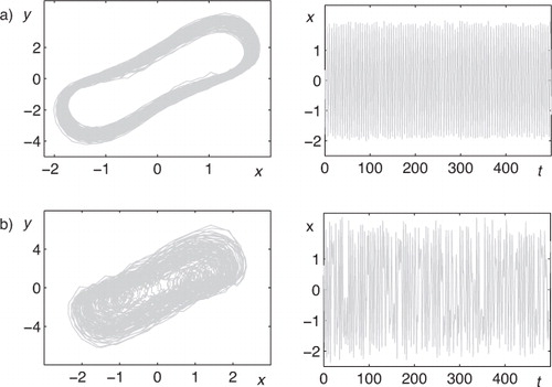
Fig. 14 Plot of k(ɛ).

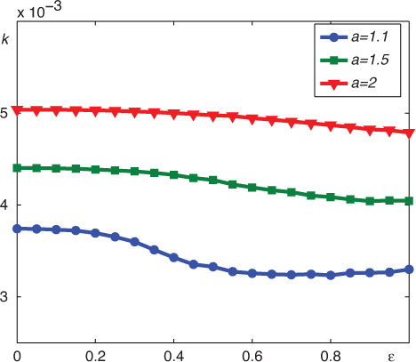
Fig. 15 Probability density function for a=1.1 and (a) ɛ=0.2; (b) ɛ=1.

It is worth noting that for the whole interval 0<a<2, under the random disturbances the structural stabilisation of the stochastic system occurs. Indeed, the deterministic system has a number of bifurcation points separating subintervals with different combinations of attractors and repellers. Increasing noise leads to blurring a distinction between the modes and forms a unified dynamical regime with the dominating stochastic cycle.

4. Conclusion

Let us summarise in conclusion the key results of the theory under consideration. We analyse a simple climatic feedback system explained by Saltzman and previously studied in a number of works by Saltzman with co-authors (Saltzman, 1978; Saltzman and Moritz, 1980; Saltzman et al., 1981, 1982) and Nicolis (1984, 1987). The main difference of the present analysis consists of studying the system dynamics in a wider domain of model parameters. The novel results of our study lie in both the deterministic and stochastic cases of system behaviour.

A complete analysis of the deterministic model demonstrates co-existence of a stable cycle and equilibrium phase points M ₁ and M ₂. The first case of climate dynamics is described by unstable equilibria, so that the system tends to a stable cycle (Fig. 4a). The second case of system dynamics corresponds to a stable cycle and two stable equilibria (Fig. 4b–4d). Moreover, a fine structure of attraction basins existing around stable equilibria M ₁ and M ₂ is quite possible (Fig. 4e and 4f). In this case, the climatic system tends to either stable point M ₁ or M ₂ from a small vicinity of any initial phase point.

In the case of stochastic dynamics caused by temperature fluctuations, we demonstrate that a simple climatic model enables the noise-induced transitions between possible system attractors. A limit (stable) cycle and two equilibria showing a possible localisation of the climate (Fig. 7a) transform to a phase system with plausible unidirectional stochastic transition from a limit cycle to one of equilibria with increasing intensity of random disturbances (Fig. 7b). Then, by further increasing the noise intensity, two-sided phase transitions from a cycle to equilibria and vice versa become permissible (Fig. 7c). Note that variation of system parameters leads to another type of one-sided transition from equilibria to a stable cycle (Fig. 8). What is more, the case of stochastic generation of large-amplitude oscillations, when noise-induced transitions occur between equilibrium points in the absence of a limit cycle is revealed as well (Fig. 10b and 10c). In this case, the climatic system moves along stochastic trajectories between equilibrium points with lower and greater mean ocean temperatures.

5. Acknowledgements

This work was supported by the Ministry of Education and Science of the Russian Federation under the project N 315.

6. Appendix. Stochastic sensitivity functions technique

Consider a non-linear stochastic system5

Here, x is an n-vector, f(x) is an n-vector function, σ(x) is an n×n-matrix-valued function of the disturbances with intensity ɛ, and w(t) is an n-dimensional Wiener process.

It is supposed that the deterministic system (5) (ɛ=0) has an exponentially stable attractor.

Random trajectories of the system (5) form a stochastic attractor with stationary probability distribution ρ(x, ɛ).

For weak noise, in a small neighbourhood of the equilibrium , one can write an approximation of ρ(x, ɛ) in the Gaussian form:

with the covariance matrix ɛ ² W. For the exponentially stable equilibrium , the stochastic sensitivity matrix W is a unique solution of the matrix equation

This matrix characterises a spatial arrangement and size of the stationary distributed random states of the stochastic system (5) around the deterministic equilibrium (Bashkirtseva and Ryashko, 2011). For the 2D-case, using this matrix, one can construct a confidence ellipse:

where r ²=−ln(1−P), and P is the fiducial probability. Let be eigenvalues and u ₁, u ₂ be normalised eigenvectors of the stochastic sensitivity matrix W. For the coordinates , the equation of the confidence ellipse can be written in a standard form:

The 2D-deterministic system has an exponentially stable limit cycle defined by the T-periodic solution x=ξ(t). In this case, the Gaussian approximation of the stationary probabilistic distribution around this cycle in the Poincare section Π _t can be written as

where Π _t is a line orthogonal to the cycle at the point ξ(t), and the scalar stochastic sensitivity function m(t) satisfies the following boundary problem

with T-periodic coefficients

where u(t) is a normalised vector orthogonal to f(ξ(t)).The value M=max m(t), t∈[0, T] is a stochastic sensitivity factor of the cycle as a whole.

The function m(t) allows us to construct a confidence band around the deterministic cycle. Boundaries x _1,2(t) of the confidence band can be written in the explicit parametrical form:

where r=erf⁻¹(P), , and P is the fiducial probability.

Stochastic sensitivity function technique was successfully applied to the analysis of noise-induced chaos (Bashkirtseva et al., 2012) stochastic bifurcations (Bashkirtseva et al., 2010) and stochastic excitability (Bashkirtseva et al., 2013).