Gaussian anamorphosis in the analysis step of the EnKF: a joint state-variable/observation approach

Abstract

The analysis step of the (ensemble) Kalman filter is optimal when (1) the distribution of the background is Gaussian, (2) state variables and observations are related via a linear operator, and (3) the observational error is of additive nature and has Gaussian distribution. When these conditions are largely violated, a pre-processing step known as Gaussian anamorphosis (GA) can be applied. The objective of this procedure is to obtain state variables and observations that better fulfil the Gaussianity conditions in some sense. In this work we analyse GA from a joint perspective, paying attention to the effects of transformations in the joint state-variable/observation space. First, we study transformations for state variables and observations that are independent from each other. Then, we introduce a targeted joint transformation with the objective to obtain joint Gaussianity in the transformed space. We focus primarily in the univariate case, and briefly comment on the multivariate one. A key point of this paper is that, when (1)–(3) are violated, using the analysis step of the EnKF will not recover the exact posterior density in spite of any transformations one may perform. These transformations, however, provide approximations of different quality to the Bayesian solution of the problem. Using an example in which the Bayesian posterior can be analytically computed, we assess the quality of the analysis distributions generated after applying the EnKF analysis step in conjunction with different GA options. The value of the targeted joint transformation is particularly clear for the case when the prior is Gaussian, the marginal density for the observations is close to Gaussian, and the likelihood is a Gaussian mixture.

• Gaussian anamorphosis
• ensemble Kalman filter
• nonlinearity
• joint transformations
• non-Gaussianity

1. Introduction

It is often the case, when estimating a variable of interest, that one only counts with imperfect sources of information. For example, to determine the value of an atmospheric variable at a given location, one can rely on a short-term forecast and observations of the variable, both of which contain errors. Data assimilation (DA) is the process of combining these sources of information in a way that is optimal in some predefined sense (see e.g. Cohn, 1997).

This paper deals with a particular aspect of sequential DA methods. These methods have two steps. In the forecast step, the state estimator is evolved in time following some dynamical model, along with some measure of its uncertainty. Whenever an observation becomes available, the information from this observation is combined with that provided by the forecast (also called background) to produce a better estimate (denominated analysis). This is known as the analysis step.

In the present work we focus only on the latter step. Hence, we consider that when an observation arrives we have already got a background estimate (regardless of the way this was obtained). We consider both the background and the observations to contain random errors with some prescribed probability density functions (pdf's). Under such a probabilistic framework, the aim of the analysis step is to obtain the posterior pdf of the variable of interest. In theory, this can be achieved through a direct application of Bayes theorem. Nonetheless, in practice this can result in a difficult task since a complete representation of the distributions for the prior and the likelihood is required.

When dealing with full pdf's is not possible, one can work with summary statistics for both the background and the likelihood. For example, the analysis equations of the Kalman filter (KF: Kalman, 1960; Kalman and Bucy, 1961) provide a method to update the first two moments (mean and covariance) of the state variable from background to analysis. In large-scale applications, such as numerical weather prediction (NWP) or oceanography, the background statistics are usually obtained from samples [ensemble Kalman filter (EnKF) Evensen, 2006].

Under special conditions: (1) Gaussianity in the prior, (2) linearity of the observation operator and (3) Gaussianity in the additive observational error density, the solution given by the analysis step of the KF/EnKF provides the sufficient statistics of the Bayesian solution (the sampling nature of the EnKF obviously introduces statistical error in this case). If these conditions are not fulfilled, the application of the (En)KF analysis equations is suboptimal, but it can still be useful.

In some cases, however, the deviation from these conditions can be quite important. This happens, for example, when the prior is multimodal or when it does not have the statistical support (domain) of the Gaussian distribution. The latter is the case of positive definite variables such as precipitation (see e.g. Lien et al., 2013), and bounded quantities such as relative humidity. Large deviations from Gaussianity in the prior are not uncommon in many fields, for example in physical–biological models (Bertino et al., 2003; Simon and Bertino, 2009; Beal et al., 2010; Doron et al., 2011). Non-Gaussian pdf's can also result from the deformation of an original Gaussian pdf during the forecast step when the model is strongly nonlinear (Miller et al., 1994, 1999). Problems can also arise if the likelihood presents extreme non-Gaussian features.

In these cases, either of two options can be taken. One can select an analysis step based on methods that do not require Gaussianity, e.g. the rank histogram filter (Anderson, 2010). On the other hand, one can still apply the (En)KF analysis step, in conjunction with a procedure known as Gaussian anamorphosis (GA). This involves transforming the state variable and observations {x, y} into new variables which present Gaussian features (details will be given in Section 3). The (En)KF analysis equations are computed using the new variables, and the resulting analysis is mapped back into the original space using the inverse of the transformation. GA is a well-known technique in the geostatistics community (see e.g. Wackernagel, 2003), and it was introduced to the DA community in a seminal paper by Bertino et al. (2003). Since then, it has been explored in different works (e.g. Zhou et al., 2011; Brankart et al., 2012; Simon and Bertino, 2012).

A possible drawback of anamorphosis is that as a result of the transformations (generally nonlinear), an observation operator is introduced in the new space (Bocquet et al., 2010). Although one can apply the EnKF with nonlinear observation operators (see e.g. Hunt et al., 2007), it seems undesirable to solve one problem (non-Gaussianity) at the cost of creating another. A central idea in this work is that different transformations in the state variable and/or observations can achieve different objectives: marginal Gaussianity in the state variables, marginal Gaussianity in the observations, joint Gaussianity in the pair {state variable, observation}. As we will see, different transformations will bring different side effects. Is there an optimal strategy to follow when performing anamorphosis? If not, how do different transformations compare? These questions are at the heart of this paper.

This paper has three main objectives. The first is to study anamorphosis transformations using a joint statistical approach between state variables and observations. The second is to visualise the effect that different transformations have on the joint probability space in which the EnKF is used. The third is to introduce a targeted joint state-variable/observation transformation which maps the pair of an arbitrary prior probability and arbitrary likelihood into a joint Gaussian space. In order to assess the performance of the different transformations, we choose an example in which we are able to compute analytically the posterior pdf of the model variables for different given observations. It is against these exact posteriors that we compare the EnKF-generated analysis pdf's.

The rest of this paper is organised as follows: Section 2 discusses the DA analysis step in more detail, the probabilistic formulation and the EnKF solution. Section 3 introduces and explains the concept of GA. Section 4 discusses the implementation of GA, studying the existing methods and introducing a newly targeted joint state-variable/observation transformation. In Section 5 we perform study cases of the methods discussed in Section 4. Section 6 includes the conclusions and some discussion.

Some remarks on notation will be useful before starting. We will try to follow (sometimes loosely) the convention of Ide et al. (1997) with respect to sequential DA. Pdf's will be denoted as , while cumulative density functions (cdf's) will be denoted as . If we want to explicitly include the parameters when referring to any distribution, this will be done with a semicolon in the argument, e.g. . The symbol ~ should be read ‘distributed as’. We will use E _x to denote expected value, with the subindex indicating the pdf with respect to which this operation is computed. For example,1

Similarly, denotes covariance, with the same meaning for the subindex. The Gaussian distribution will appear frequently in this work. For the sake of brevity, if the random variable (rv) follows a Gaussian distribution with mean and variance σ² _ξ, we will denote its pdf as:2

and its cdf as:3

For some examples, we will also use exponential rv's. The pdf for this distribution is:4

where is a scale factor.

2. Analysis step: Bayesian and EnKF solutions

In this section, we make use of transformations of rv's; basic concepts of this topic can be found in Appendix A. Let denote the vector of state variables, and consider it follows a prior distribution . In the most general case, the observations follow the relationship:5

where is a nonlinear observation operator, and represents the observational error, which follows a distribution p _η ( η ). Consider there exists an inverse (as a function of y), then the likelihood – conditional pdf of y given x – can be written as:6

where is the absolute value of the determinant of the Jacobian matrix of the transformation. The joint pdf of x and y is the product of the likelihood and the prior. The posterior distribution can be computed via Bayes’ theorem as:7

The denominator p _y (y) is the marginal pdf of the observations, and can often be treated as a normalisation factor of the posterior pdf, since it does not depend on x.

This is the most general solution for the DA analysis step. Nonetheless, obtaining the posterior pdf is not an easy task in many occasions, since it requires full knowledge of the two densities involved in the product of the numerator of eq. (7). Let us step back and discuss a considerably simpler case; we will build on more complicated cases later. Hence, let eq. (5) become:8

where is a linear operator and the observational error is additive. Define , (denoted in the univariate case), (denoted in the univariate case), and . One can get a minimum variance estimator for the analysis mean as:9

where is known as gain, and is computed as:10

The covariance of the analysis is computed as:11

Expressions (9) and (11) are the KF analysis equations (Kalman, 1960; Kalman and Bucy, 1961). If, besides having a linear observation operator and additive observational error, both p _x (x) and are multivariate Gaussians, then using these equations is optimal. This means they produce the sufficient statistics of the full Bayesian posterior. Note that if the set {x, y} has a joint multivariate Gaussian distribution, then the aforementioned conditions are automatically fulfilled.

It is important to mention that the marginal pdf of the observations is , again a multivariate Gaussian, this time with mean and covariance:12

Now, let us partially relax the assumptions on the likelihood. For nonlinear observation operators and additive error, the observation equation is:13

It should be clear that in this case eq. (6) simplifies to . A first order (linear) approximation to the KF analysis equations, known as extended KF (EKF, see e.g. Jazwinski, 1970) can be written as:14

where is the tangent linear operator of h, i.e. the Jacobian matrix .

Formulating the KF analysis equations for a general observation operator as indicated in eq. (5) is much more complicated (and further away from optimal conditions), since it would require the linearisation of with respect to η to express:15

This approximation of course will only be accurate for small η.

To end this section, it is useful to discuss the analysis step of the EnKF (see e.g. Evensen, 2006). This is a Monte Carlo implementation of the KF, and uses sample statistics. Let us denote the background ensemble as , where . The sample mean is:16

An ensemble of perturbations around the mean can be defined as: , where . Then, the sample covariance is:17

The KF analysis equations update both mean and covariance, but in the analysis step of the EnKF it is necessary to update each one of the M ensemble members. This can be done deterministically (ensemble square root filters: Tippett et al., 2003), or stochastically (perturbed-observations EnKF; Burgers et al., 1998). In this work we focus on the stochastic formulation (henceforth EnKF will refer to perturbed-observations EnKF), where each ensemble member is updated as:18

where K is defined as before but using the sample covariances, and the perturbed observations {y _m } are samples from . In particular, if the error is additive they relate to the actual observations by y _m =y+ η _m , where η _m is a particular realisation of the observational error. By construction, the KF analysis equation for the mean is fulfilled if the perturbed observations are generated such that , where is the sample mean. The KF analysis equation for the covariance is fulfilled in an statistical sense.

In the case of nonlinear observation operator, eq. (18) would be written as19

In the EKF analysis equation, the computation of involves calculating . In the analysis step of the EnKF one can avoid computing this Jacobian by using the ensemble (Hunt et al., 2007). First, one maps into observational space using the nonlinear observation operator to get a new ensemble . Explicitly:20

Then a sample mean can be computed, as well as an ensemble of perturbations around this mean . Finally, is computed as:21

For the EnKF analysis step, the quality of the sample estimators does depend on the ensemble size M, and this size should be related to the number of unstable modes in the model. It is not within the objectives of this paper to consider the effect of ensemble size, since what we want to evaluate is the exact solution produced by the analysis step of the EnKF when computed in different spaces, and how does it compare to the actual Bayesian posterior. For this reason, we will consider effectively infinite ensemble size ( in all our experiments) such that and .

3. Anamorphosis

In Section 1, we stated three conditions that ensured optimality in the application of the (En)KF analysis step. For the moment, let us assume that conditions (2) and (3) are fulfilled, and focus on non-Gaussian priors. Two cases – for – that result as challenging for the application of the EnKF analysis step are illustrated in Fig. 1. In both cases, the likelihood has been kept Gaussian and centred at the (directly observed) state variable.

Fig. 1 Comparison of the analysis pdfs obtained by a direct application of the EnKF analysis step (green line) with respect to the actual Bayesian posteriors (magenta line). The state variables have either a multimodal prior distribution (left), or they are positive–definite quantities (right). The EnKF analysis step is applied with M=10⁶.

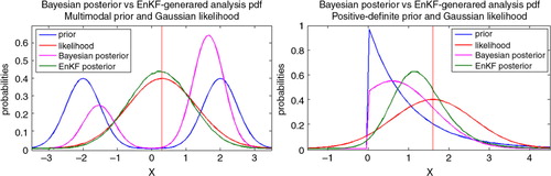
In the left panel, the prior (blue line) is bimodal, a mixture of two Gaussians centred in x= − 2 and x=2 with equal variance σ²=. The prior mean is x=0, corresponding to a region where p _x (x) is close to zero. By assimilating an observation (red line) at y = x=, the EnKF incorrectly constructs a unimodal analysis pdf (green line) which does not resemble at all the Bayesian posterior (magenta line). In fact, the analysis pdf is centred in a region where the posterior pdf is close to zero.

In the right panel, the prior is an exponential distribution with . This is a positive–definite variable, and the Bayesian posterior (corresponding to an observation at y=x=) correctly captures this information, since . The analysis pdf given by the KF, however, yields non-zero probabilities for negative values of x. In reality, physical observations of a non-negative variable will not be negative. An additive error with Gaussian distribution cannot be used in practice: either a truncated non-symmetric distribution is likely to be used, or negative values will be mapped to zero. Moreover, in these cases the nature of the observational error tends not be additive, but multiplicative for instance. Nonetheless, for the purpose of illustration, we allow the existence of negative observations.

To avoid the mentioned problems, one can transform the state variable before applying the EnKF. The ultimate goal of this procedure is to map x, a variable with an arbitrary multivariate pdf p _x (x), into a new state variable with multivariate Gaussian pdf . Then, the KF analysis equations can be applied to the transformed variables, and these updated values can be mapped back into the original space. This mapping process is known as GA.

In the univariate case (), applying GA is conceptually not complicated (aside from the implementation aspects). One could use analytic functions such as logarithm or Box–Cox transformations, but these are not guaranteed to improve the distribution in general (Simon and Bertino, 2009). A better solution is to make use of the integral probability transform theorem (IPT) and solve for the new variable as (for details see Appendix A):22

The moments of the target Gaussian variable are set to be those of the original ensemble (see Section 4.4 Bertino et al., 2003). Of course, in the implementation one can transform x into a standard Gaussian rv N(0,1), and then translate and scale the values correspondingly to get .

The actual prior p _x (x), and consequently the cdf P _x (x), are rarely known perfectly. Hence, to apply the IPT, the first step is to empirically estimate P _x (x). This can be done using the ensemble. Then, a set of percentiles of this empirical cdf are mapped to the same percentiles of the cdf of a target normal distribution. A piecewise linear transformation can be used to get the intermediate values, and special care has to be taken when dealing with the tails (Simon and Bertino, 2009; Beal et al., 2010). The quality in the estimation of P _x (x) clearly depends on the size of the ensemble. In order to increase the sample size, one can make use of values of the variable at different times and consider a stationary climatological pdf. Refinements to this idea include time-evolving anamorphosis functions. Simon and Bertino (2009), for example, construct the GA function for the state variables from a window of 3 months centred on the datum in a 3-D ecosystem model.

The multivariate case is considerably more difficult. Strictly speaking, it requires a joint multivariate transformation. A multivariate version of the IPT exists (Genest and Rivest, 2001), but its application is not simple. Besides, checking for the joint Gaussianity of a multivariate spatial law is quite computationally demanding (Bertino et al., 2003). For this reason, implementation of GA in large models is often done univariately, i.e. a different function is applied for each one of the components in the state-variable vector:23

For field variables, one can either consider them to have homogeneous distributions, or one can apply local anamorphosis functions at different gridpoints (Doron et al., 2011; Zhou et al., 2011). Another option for the multivariate case is to rotate the space to get uncorrelated variables by performing principal components analysis (PCA). It is not straightforward, however, that the updated variables will follow the same PCA, since the transformations are nonlinear (see the discussion in Bocquet et al., 2010). Moreover, residual correlations may remain (Pires and Perdigao, 2007). A more complicated approach involving copulas has been suggested by Scholzel and Freidrichs (2008).

Up to this moment we have only considered transformations of the prior, but the observations can be transformed as part of a more general GA process, i.e.24

In the transformed space, y˜ and are related by the observation operator25

where ○ denotes function composition. In this space, for each one of the transformed ensemble members, the EnKF analysis value can be obtained as (Bertino et al., 2003):26

To compute y˜ _m , Simon and Bertino (2012) propose to perturb the observations in the original space by sampling from , and then map each of the perturbed observations individually . In this work we use said approach. The perturbed variables have associated covariance matrices and , which can be computed directly from the ensembles and . These covariance matrices are used for the computation of . If is nonlinear, then one uses the same procedure described at the end of Section 2 for the computation of .

A crucial issue in GA is the choice of the transformations g _model (·) and g _obs (·), and the effect these choices will have in the observation operator in transformed space. In the next section, we study different choices for these maps.

4. Choosing anamorphosis functions

We now discuss different ways to transform {x, y} into new variables , paying attention to the effects these transformations cause in the joint characteristics of state and observations. Is there a transformation that produces a Gaussian posterior in the transformed space? The search for this ideal case leads this section.

For the moment, we focus on the univariate case (). We start with a generalisation of eq. (24) and consider joint bivariate forward transformations of the form:27

with the respective backward transformations:28

Then, if the joint pdf of {x, y} in the original space is , the joint pdf in the transformed space is (see Appendix A for details):29

We will now study different choices for eq. (27). Throughout the rest of this section, we will use the following example to visualise the effects of these choices in the joint state-variable/observation space. The prior pdf, likelihood, and observation equation are [refer to eq. (2) for notation on Gaussian rv's]:30

Both pdfs are Gaussian mixtures (GMs) with expected values equal to 0; p _x (x) is symmetric while p _η (η) is not. One can think of this choice for p _x (x) to be plausible, but this type of distribution is rarely used for observational error. It could be seen as the result of the interaction of a simpler likelihood with a nonlinear observation operator. In any case, using GMs is convenient since they allow tractability of the analytical Bayesian posteriors (see Appendix B for details), something very useful for illustration and evaluation purposes. Also, GMs can be used to approximate any smooth pdf.

The application of different anamorphosis functions for this example is illustrated in Fig. 2. This figure has five panels, one for each transformation. In every panel we show the joint bivariate distribution of the state variables and observations (contour plot), the marginal distribution of the state variable (horizontal plot) and the marginal distribution of the observations (vertical plot). Also, we consider individual given observations (shown as colour lines on top of the bivariate plot), and the effects of the transformations in these observations.

Fig. 2 Bivariate distributions (contour plots) and marginal distributions (line plots) for state variables (horizontal) and observations (vertical) under six different transformations [panels (a)–(e)] described in the text. Individual given observations are identified with colour lines in the contour plot, except for panel (f) where individual values of x are shown.

4.1. Independent transformations

The simplest case is to make the transformations for state variables and observations independent. This means and . Then, eq. (29) simplifies to:31

Next, we list some choices for independent univariate transformations.

(a) Working in the original space.

In this trivial case, both transformations are the identity:32

This amounts to just applying the EnKF in the original space, but it serves as a benchmark for comparison. As we see in panel (a) of Fig. 2, for our example both and are bimodal, with showing asymmetry, a consequence of the asymmetric likelihood. In the joint state-variables/observations space, this translates into two sell-separated areas of high probability. This is indeed a scenario that ensures non-optimality for the use of the EnKF.

(b) Transforming only x.

In this case, only the state variable is transformed into a Gaussian rv. Hence the transformations are:33

where explicitly indicates that the cdf in transformed space is that of a Gaussian rv (see notation defined in Section 1). As we can see in panel (b) of Fig. 2, this transformation achieves a marginal Gaussian , but does nothing either on or in the individual observation values. The joint pdf does not show the isolated peaks as before, but instead it has elongated features, a consequence of populating regions of the space variable around 0 which were previously unpopulated.

(c) Transforming both x and y with the same function.

This transformation is only possible when the domains of x and y are the same, as in our example with h=1. This option cannot always be applied; it would be incorrect, e.g. if and . For the sake of completeness, we include it in our discussion. In this case the maps would be:34

The application of this transformation in y does not guarantee anything characteristic for . Panel (c) of Fig. 2 illustrates the effect of this transformation. While the state variable is indeed transformed into a Gaussian, we obtain a non-Gaussian and very peaked distribution for , which translates in a very narrow bivariate pdf with respect to y˜. The individual observations are transformed, as depicted by the colour lines.

(d) Transforming x and y marginally.

With the previous methods one achieved marginal Gaussianity in , but not on [ytilde]. One can apply the IPT to y and obtain marginal Gaussianity in [ytilde]. The maps would then be:35

This transformation involves knowing the marginal distribution of the observations, or at least constructing an estimation. This is the approach used in Simon and Bertino (2009, 2012). In these works, the authors estimate a marginal climatological pdf for observations using values from an extended time period. Panel (d) of Fig. 2 shows the effects of this transformation. As we can see, both marginal pdf's are Gaussian. The individual observations are transformed [as in panel (c)]. The joint pdf, however, looks very different from a bivariate Gaussian; recall that whereas bivariate Gaussianity implies marginal Gaussians, the opposite is not true (e.g. Casella and Berger, 2002).

4.2. Joint state-variable/observation transformations

In Section 4.1, the objectives of the proposed transformations became progressively more ambitious. The last case achieves marginal Gaussianity in both and [ytilde]. Still, with independent transformations we are not able to guarantee any particular characteristics for the relationship between state variables and observations in the transformed space. We now introduce a joint state-variable/observation transformation which has precisely this objective: to transform the pair {x, y} (with arbitrary joint pdf) into the pair (with joint Gaussian pdf). Consequently as a by-product, the marginal and conditional pdfs in this space will also be Gaussian. Our algorithm can be divided into three steps. These are listed next and also depicted in Fig. 3.

Fig. 3 The process for the joint state-space/observations transformation described in Section 4.2. First (i), a target probability space is constructed using the statistical moments inferred or prescribed by the original variables. Second (ii), the state variables (both original and transformed) are mapped into a random variable w distributed U[0,1]. Finally (iii), for each w an equation of cumulative likelihoods is solved to find y˜ in terms of y.

(1) The first step corresponds to the upper row of Fig. 3. In this step we pre-design a transformed space (right panel) which is joint Gaussian and that shares statistical characteristics with the original space (left panel). In the transformed space we set the prior as , and the likelihood as . The moments of are estimated by the sample moments of the ensemble in the original space, i.e. , and the observational error is prescribed (or deduced) from the original likelihood, i.e. . is a linear observation operator (in our example we choose the identity).

(2) The second step corresponds to the middle row of Fig. 3. We map both x and into w~U [0, 1], i.e. an rv with uniform distribution in the interval [0, 1]. Simply applying the IPT to both variables does this:36

The previous procedure is just the application of eq. (22) with an extra intermediate step. Let us focus on the spaces {w, y} and {w, [ytilde]}. Since the marginal pdf of w is simply p _w (w)=1 I _{[0, 1]}(w)–where I _{[0, 1]}(·) is the indicator function–, the joint pdf p _w,y (w,y) coincides with the conditional pdf , i.e. . The same applies to the {w,[ytilde]} case, i.e. .

For our example, these distributions are illustrated in the second row of Fig. 3, and they are shown in better detail in Fig. 4. In the left panel of this figure we depict p _w,y (w,y), the centre panel depicts p _w,[ytilde] (w,[ytilde]) and the right panel is the difference between the two [we can do this subtraction because y and [ytilde] have the same support ]. In the left panel, we can see the effect of having a GM as prior, as we can see two well-separated regions in the joint pdf, with a division at w=0.5. We can also notice the effect of the non-symmetric likelihood: the distance between the contours in the upper part of the coloured strip is less than the distance between those in the lower part. These effects are not present in the centre panel. In fact, we need a way to convert the left panel into the centre panel; this is the purpose of the next step.

Fig. 4 Joint pdfs for the spaces {w, y} (left) and {w,[ytilde]} (centre). The difference between the two densities is plotted in the right panel.

(3) The last step is depicted in the bottom row of Fig. 3. For the last step we design a transformation from y to y˜ such that the given p _w,y (w,y) becomes the prescribed . This is equivalent – as we have explained before – to transforming into . Hence, for each and every value of w, we can state the following equation of cumulative likelihoods:37

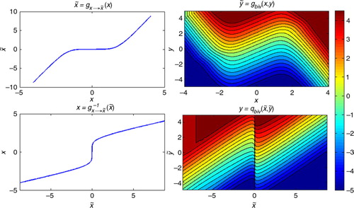
Although it is not always possible to obtain explicitly, the solution of this equation is of the form [ytilde]=[ytilde](w,y). Solving this equation for each and every value of w completes the construction of the map from {x,y} into . To summarise, the transformation we just devised is formed by the forward and backward maps:38

In Fig. 5, we show the form of these maps in our study case: forward transformations in the top row and backward transformations in the bottom row. The top left panel shows the simple IPT-based transformation from x to . For the region −1 < x<1, the graph looks almost horizontal, but it is not. This consequence comes from the fact that in this region p _x (x) is close to zero, while this same region contains the largest probability mass for , so the slope of the map in this region is extremely small. The top right figure shows the joint transformation [ytilde]=[ytilde](x,y), which is the solution of eq. (37) in terms of y and w, but with the values of w replaced by the corresponding x for the plot. The bottom left panel shows the transformation from to x. Again, it is a simple IPT-based implementation. This time we observe an almost vertical behaviour of the graph near , for the reasons stated before. On the other hand is the solution of eq. (38) in terms of y and w, with the values of w replaced by the corresponding values of for the plot. The plot would suggest a discontinuity around , but this is not the case, as there is only a sharp change not captured at the resolution of the graph. This behaviour is associated with the characteristics around x=0 previously described.

Fig. 5 Joint bivariate transformations from the {x,y} space (with GM marginals) to the space (with a joint bivariate Gaussian pdf). The first row shows the forward transformations: the state variable is univariately transformed (left) whereas the observation is transformed in a joint bivariately manner (right). The backward transformations are presented in the bottom row.

The method we just described can be considered a special instance of the multivariate Rosenblatt transform (1952). Furthermore, the statistical characteristics of the joint state-variable/observation space constructed with this method fulfil conditions (1)–(3). At first sight, one could consider this to be an optimal transformation. Things are not that simple, however, and the complication comes from the mapping of the given individual observations. The issue is that a fixed value y ₀ in {x,y} is not fixed anymore in , it becomes a function (actually a function of x since y ₀ is a fixed value). This can easily be seen in panel (e) of Fig. 2. By construction the obtained joint distribution is bivariate Gaussian (and consequently the marginals are Gaussian as well), but fixed observations are no longer horizontal lines, instead their values depend on . This leads to a conceptual complication: in the space we are not finding a posterior in the proper sense (or estimating its first two moments, since we are using the EnKF). In this space, the posterior is the pdf along a horizontal line of fixed [ytilde]. But we do not have fixed [ytilde]'s, instead we have functions. Does this mean we are actually estimating a probability of the form instead of ? This may not be as big a problem if we individually update each ensemble member (as we do), it would be more problematic if we were using a deterministic square root filter, updating mean and covariance, and constructing the ensemble members after that. Fortunately, by using perturbed observations we sample directly from the likelihood. This avoids bias, as indicated in Simon and Bertino (2009). Finally, it is important to mention that if we wanted the Bayesian solution in the transformed space we would need to compute the corresponding normalisation factor, in this case , which cannot be considered a constant with respect to . Fortunately, we do not require this factor after mapping the sample back to the original space.

The EnKF analysis equation in the transformed space is simply eq. (18), and it is linear. For we use the sample covariance in transformed space. The observational error variance is prescribed based on the characteristics of the likelihood in the original space. One could compute the empirical observational covariance in the transformed space, but one could not be averaging over straight lines, but functions of (see the previous discussion). Hence, this could lead to an overestimation or underestimation of the actual observational covariance.

4.3. Transformations in the multivariate case

Performing GA in the multivariate case ( and ) is considerably more difficult. As mentioned in Section 3, the simplest way is to do independent transformations for each one of the state variables [see eq. (23)] and observations. If there are variables that are neither transformed nor observed, they are still affected by the transformations via the corresponding covariances. For illustration, consider a two-variable system in which the first variable is indirectly observed, i.e. and y=[y ₁]=[h(x ₁,η ₁)]. Even if the unobserved x ₂ is not transformed, the update from background to analysis of this variable is different in the original space than in one in which a GA of the form is performed. We can see this if we develop explicitly eq. (19) for this variable in the two cases:39

where and . The anamorphosis functions should guarantee that and that . Hence, the crucial part is the way in which the anamorphosis function changes the covariance between the observed and the unobserved variable. This is, the change from to .

Now, let us think again about targeted joint transformations. Following our rationale in Section 4.2, the ultimate goal in this case would be to go from the space {x,y} with a general nonlinear operator h to a space with a joint multivariate distribution and a linear observation operator . This may not be possible in general, depending on the precise behaviour of h.

For the moment, we can propose a modest solution. Let us consider that there is a set of L variables that are observed as: . Then, we can perform the proposed joint transformations for each pair . The effect of these transformation into other variables will still be communicated through covariance, just as in eq. (39). To explore the full problem, one could start with a simple system such as the one described in this subsection (two variables: one observed, one not). Can we replace a joint trivariate transformation by a sequence of two joint bivariate ones? This is one of the ideas we are exploring at the moment.

5. Experiments

In this section, we study the analysis pdf's that result from performing the EnKF analysis step in combination with the transformations described earlier. For the sake of brevity, we will take the following short notation when describing the five spaces in which the EnKF analysis step is applied. Its application in {x, y} is denoted as K{x,y}, in {[xtilde]=g _{x →x˜}(x), y}→ as , in as , in as , and finally in as .

Figure 6 shows the results of assimilating an observation at in the system [eq. (30)]. The true Bayesian posterior (black line) is bimodal, with a considerably taller peak in the negative values. The analysis pdf produced by K{x, y} (blue line) does not resemble this at all, instead it generates a pdf centred close to zero with a hint of bimodality. Note that a Gaussian analysis pdf is not produced (as it was the case in the left panel of Fig. 1) because in the current experiment the likelihood is not Gaussian and the perturbed observations were produced using the correct likelihood.

Fig. 6 Comparison of the Bayesian posterior distribution (black line) with respect to the EnKF-generated analysis pdfs, with the EnKF analysis step applied in five different spaces (colour lines) for a given observation (dotted vertical line). Both the prior and likelihood in the original space are GMs.

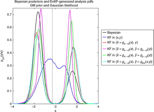
For the other five cases the resulting empirical posteriors are indeed bimodal. (magenta line) produces almost symmetric peaks. (green line) gives more probability to the wrong mode. (red line) and the bivariate transformation (cyan line) gives higher probability to the left peak, resembling the actual Bayesian posterior.

5.1. An objective assessment of the quality of the EnKF-generated analysis

The previous discussion was rather qualitative. We now use the Kullback–Leibler divergence (D _KL , see Cover and Thomas, 2006) to quantitatively compare the EnKF-generated analysis pdfs with respect to the Bayesian posteriors. For two continuous pdfs p(x) and q(x), this quantity is defined as:40

The definition for D _KL can be interpreted as the expected value of the logarithmic difference between the probabilities p(·) and q(·), evaluated over p(·). D _KL quantifies the information gain from q to p (Bocquet et al., 2010). Note that , and D _KL (p,q)=0 if and only if the two densities are equal almost everywhere. Roughly speaking, the larger the value of this quantity the more different the two distributions are. In our case, p(x) is the exact Bayesian posterior, whereas q(x) is the EnKF-generated analysis pdf. We compute the D _KL numerically after dividing the data in J _bins bins, and using the following expression:41

We will consider an experimental setting which stems from a generalisation of the system [eq. (30)]. The prior and (additive) observational error pdf's are:42

and the observation operator is the identity. We will choose three combinations of parameters:

(1) The prior is a GM and the likelihood is Gaussian (GM–G).43 (2) Both the prior and the likelihood are GMs (GM–GM).44 (3) The prior is Gaussian and the likelihood is a GM (G–GM).45

Furthermore, recall that we are assessing the quality of the empirical distributions that approximate , which depend on a given observation. The Bayesian posterior and the analysis pdfs generated by the EnKF analysis step – which were plotted in Fig. 6 – were based on a single observation. For the current experiment, however, we reconstruct the distributions for a range of 21 different observation values. For each one of the three scenarios (a–c), for each one of the five transformations, and each one of the 21 given observations we compute D _KL . We plot this information in the left panels of Fig. 7, a different colour for each different transformation. In this figure, the top row corresponds to the GM–G case, the centre row to the GM–GM case and the bottom row corresponds to the G–GM case. Of the 21 observation values we select three, which we identify with the violet, black and orange vertical dotted lines in these panels. In the right panels we take those observations and plot the Bayesian posteriors associated to them, each Bayesian posterior is identified with the corresponding colour. The quality of the EnKF-generated analysis distributions in the five different spaces will depend on the shape of the real Bayesian posterior they are trying to emulate. This is discussed in detail for each scenario.

Fig. 7 Assessing the quality of the EnKF-generated analysis pdf's for three cases: GM–G (top row), GM–GM (centre row) and G–GM (bottom row). The left panels shows the D _KL for the EnKF-generated analysis pdf's with respect to the Bayesian posterior (coloured lines) for different given observations (horizontal axis). In each case we choose three given observations (vertical lines with markers) and in the right panels we show the Bayesian posteriors associated with those three observations (coloured lines with markers, the colours correspond to those of the vertical lines). The solid grey curve in these panels represents the prior for each case.

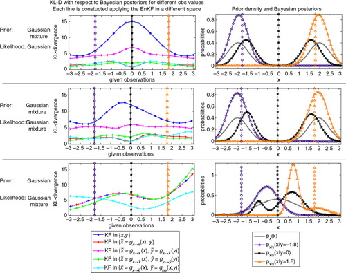
(1) Let us start with the GM–G case in the top row. Because of the settings (a bimodal prior symmetric with respect to x=0 and a Gaussian likelihood), we expect equal to . This is indeed what we get for the five methods. For all the values of the observation, it is clear that K{x, y} is the worst method. In particular, its highest D _KL value is for y ₀=0 (vertical black line), since this y ₀ gives rise to a bimodal posterior (black curve in right panel), a definite challenge for the EnKF applied in the original space. For the other two observational values (y ₀= − 1.8 violet line, and y ₀=1.8 orange line), the posteriors are close to Gaussians, and hence the D _KL values are lower. The next largest D _KL corresponds to . Again, the worst performance is for y ₀=0, but there is a consistent gap for all observational values between this and the other methods. The D _KL values for the other three methods are very close. The performance of both and is almost indistinguishable for all values of observations. In the interval is outperformed by and , but outside this interval it is the best method overall.

(2) In the centre row we have the GM–GM case. Not surprisingly, K{x,y} presents the worst performance, followed by , and both perform worst for observations that produce bimodal posteriors. This is again the case of y ₀=0 (black vertical line) which produces a non-symmetric bimodal posterior (right panel). The performance of and is again very close to each other. It is interesting that for −2.4 < y ₀<0.6 both and have the best performance, whereas for y ₀< − 2.4 and y ₀>0.6 the best method is . We could identify that this particular method tends to have trouble with bimodal asymmetric posteriors.

(3) Finally, we have the G–GM case in the bottom row. For this scenario, three transformations are exactly the same: K{x,y}, & . The reason for this is that the transformation is the identity (the prior is already a Gaussian). This is why in the left bottom panel of the figure one line has the three corresponding colours (blue, red and magenta); we will refer to this line simply as K{x,y}. One can immediately notice that K{x,y} and have a very similar performance for most observations. The explanation is that with the settings of this experiment the marginal p _y (y) is very close to being Gaussian, so that the transformation p _y (y) is very close to the identity again. Still this method outperforms K{x,y} for y₀<−0.4. Note that the best performance for both methods is for large negative observations; as we can see for y ₀=−1.8 (vertical violet line) the Bayesian posterior is close to a Gaussian (right panel). This is not the case, however, for the posteriors produced by y ₀=0 (black vertical line) and y ₀=1.8 (orange vertical line). As it can be seen in the right panel of this row, both Bayesian posteriors are bimodal and asymmetric (black and orange lines). In this example, we can truly appreciate the value of both bivariate transformations; for most parts of the observation values they outperform the other methods, and the difference is especially significant for the challenging cases mentioned above.

6. Summary and discussion

The analysis step of the EnKF is optimal when the following three conditions are met: (1) the distribution of the prior is Gaussian, (2) the observation operator that relates state variables and observations is linear, and (3) the observational error is additive and follows a Gaussian distribution. The analysis step of the EnKF is often applied in spite of the violation of these conditions and still yields useful results. There are cases, however, when the departure from said conditions is too considerable. In these cases, a technique known as GA is applied to convert these distributions into Gaussians before performing the analysis step.

The ultimate goal of GA would be to convert the set {x,y} of arbitrary joint distribution into the set with a joint Gaussian distribution. This is not an easy objective at all, and a proper multivariate GA transformation is not straightforward to devise. For this reason, GA is often applied in a univariate manner. Thus, we have mostly restricted ourselves to the univariate case . For this case, we have analysed GA transformations starting from the following classification: independent, i.e. transformations of the form , and joint state-variable/observation, i.e. transformations of the form .

For independent transformations (Section 4.1), we have studied some options: (1) an identity transformation – i.e. working in the original space – (denoted K{x,y}), (2) transforming only the state variable (denoted ), (3) transforming both state variables and observations using the same function –applicable only when h is the identity – (denoted ) and (4) transforming state variables and observations to obtain marginal Gaussianity for both (denoted ).

One of the contributions of this work is the introduction of a targeted joint state-variables/observation transformation (Section 4.2) of the form , which is briefly outlined next. Having original distributions p _x (x) and , we devise target Gaussian distributions and with prescribed parameters. Both p _x (x) and are mapped into an auxiliary variable . Finally, an equality of cumulative likelihoods is solved for all w and this completes the transformation .

To test these transformations, we have selected a case in which the Bayesian posterior can be obtained analytically, in particular a directly observed GM prior–GM likelihood model with three settings: GM prior with Gaussian likelihood, GM prior with GM likelihood, and Gaussian prior with GM likelihood. We have compared the posterior pdf to the pdf's generated after applying the EnKF analysis step in conjunction with the different transformations. This resemblance has been evaluated using the Kullback–Leibler divergence (D _KL ) for different given observations (Fig. 7). To further understand the behaviour of the D _KL curves, we have plotted the Bayesian posteriors for three selected observational values (right panel of the same figure).

The truth is that, despite the application of any of the different transformations, the analysis step of the EnKF cannot exactly reconstruct the Bayesian posterior when conditions (1)–(3) are not met in the original space. Still, one can get approximate solutions, and it is clear that some are better than others.

In all cases, K{x,y} has the worst performance, highlighting the fact that severe deviations from Gaussianity in both the prior and likelihood can handicap the performance of the EnKF analysis step. The next method in increasing order of performance is . It seems that, at least for the situation we studied, applying the same transformation for both state variables and observations is not an appropriate strategy. In the first two cases (GM–G, GM–GM), three methods have very similar performance: , and . What are the sources of error for each one of these two methods, i.e. in what sense is the application of the EnKF analysis step not exact? For and the answer is the appearance of a nonlinear observation operator; for is the fact that the given observations are no longer fixed values but instead functions of the state variable [recall the coloured lines in panel (e) of Fig. 2]. In these two cases we studied, these errors seem to lead to the same performance.

The real advantage of the bivariate transformation is appreciated in the G–GM case. In this case the transformation is just the identity (since x is already Gaussian), and also is very close to the identity since turns to be close to Gaussian. In this scenario, clearly outperforms the other methods when trying to reconstruct non-symmetric non-Gaussian posterior densities.

This work has two main limitations. First of all, we have considered the infinite ensemble size scenario – in fact all of our experiments were done with M=10⁶ –, which allows us to perfectly know and simulate the distributions p _x (x) and . This is of course not the case in real applications. In general, an estimation of p _x (x) has to be constructed empirically using the ensemble. The likelihood can often be considered to be prescribed (Bertino et al., 2003), but on occasions it is also necessary to construct an empirical estimation. For our bivariate method, the estimation of p _x (x) can be done with the ensemble, but in general one does require a good knowledge of the likelihood. When ensemble sizes are small and the knowledge of is not too precise, it is perhaps better to rely on a marginal transformation for both x and y [Section 4.1, method (d)]. This is because one can increase the sample size by including state variables and observations for an extended time period and consider either stationary marginal distributions, or slowly-evolving ones (Simon and Bertino, 2009).

The second limitation is that we have restricted ourselves to the univariate case, and just briefly mentioned some ideas for the multivariate one (Section 4.3). GA implementations in large models is often done univariately (e.g. Simon and Bertino, 2012). To consider several variables at once would require multivariate anamorphosis. This is indeed a challenging and on-going area of research (Scholzel and Friedrichs, 2008), and we hope that our insights on the univariate case may give guidance in the multivariate one. A further exploration of joint state variables–observations of GA transformations for multivariate cases is part of our on-going work.

A final comment must be stated. Our entire analysis has been restricted to the analysis step of the EnKF, and we have ignored any effects that the cycling of the forecast and analysis steps may bring. Therefore, the impacts of GA in forecast capabilities have not been assessed. In this sense, any benefit from the suggested transformations has not been proven. We are working towards satisfactorily answering these questions in the future.

Acknowledgements

The authors would like to acknowledge fruitful discussions with members of the Data Assimilation Research Center in Reading, in particular the members of the particle filter group. The extensive comments and reviews of three referees helped improve the presentation and content of the work considerably. The support of NERC (project number NE/I0125484/1) is kindly acknowledged.

8. Appendices

A: Transformations of random variables

Let x be a univariate random variable (rv) with pdf p _x (x). Let g be a monotonic transformation and define . The distribution of , denoted as , is given by (see e.g. Casella and Berger, 2002):46 where g ⁻¹ is the inverse of g. This inverse exists and is unique due to the monotonicity of g; if this condition is not met then one has to divide the sample space X into subsets X ₁,X ₂,…,X _k in which g is monotonic, perform the transformation in each set, and then add. One must be careful when transforming conditional probabilities. Consider . If one performs the transformation , it is clear by eq. (45) that47 On the other hand, if we still consider the same conditional probability but with the transformation , the new conditional density is simply p _y|x˜(y|x˜)=p _y|x (y|x=g⁻¹(x˜)), since the transformation is performed on the variable upon which the pdf is conditioned.

The process becomes clearer if we consider the bivariate transformation for the pair {x, y}. Let this pair have a joint distribution , and define the joint bivariate forward transformations:48 Consider these transformations to be invertible resulting in the following two backward transformations:49 Then, the transformed pair has the following joint distribution:50 where det(J) is the absolute value of the determinant of the Jacobian matrix of the transformation, namely:51 In general, a joint multivariate transformation , with , and will transform a joint pdf p _x =(x) into:52 where is the Jacobian matrix.

Another important concept to recall is the so-called integral probability theorem (IPT). If P(x) is the cdf of x, then the variable w=P(x) has uniform distribution in the interval [0, 1]. Multivariate extensions of this theorem exist, although the application is not straightforward as in the univariate case (Genest and Rivest, 2001). The IPT allows us to convert any rv into another; to transform into one can write:53 One can check eq. (51) by using eq. (45) and defining . Then:54

B: Exact Bayesian posteriors for GM priors and GM likelihoods

In this appendix, we analytically compute the marginal distribution for the observations p _y (y) and the posterior distribution for the state variable when both the prior probability and the likelihood have GM distributions. We limit the analysis to the univariate case with observation operator h=1. Following the notation for Gaussian densities introduced in the text, we have:55 The first two moments of this distribution are:56 In a similar manner, the likelihood can be expressed as:57 where the subscript η denotes the additive observational error in the observation equation y=x+η. The first two moments of the distribution are:58 where clearly . Notice that the variance is independent of x.

The joint distribution of the state variables and observations is:59

Recalling that , the marginal distribution for the observations is:60 The first two moments of this distribution are:61

Using Bayes theorem, we can compute the posterior as:62 where the subindex denotes analysis. This is again a GM, in which the weights, means and variances of each one of the J _b J _η Gaussian terms are:63

Finally, the first two moments of this posterior distribution are:64

In this paper, we have used cases in which either the prior or the likelihood are simple Gaussians. These are obviously special cases of the aforementioned solution. Gaussian likelihood corresponds to J_η =1, whereas Gaussian prior corresponds to J _b =1.

References

- Anderson J. L . A non-Gaussian ensemble filter update for data assimilation. Mon. Weather Rev. 2010; 138: 4186–4198.
- Beal D. , Brasseur P. , Brankart J.-M. , Ourmieres Y. , Verron J . Characterization of mixing errors in a coupled physical biochemical model of the North Atlantic: implications for nonlinear estimation using Gaussian anamorphosis. Ocean Sci. 2010; 6: 247–262.
- Bertino L. , Evensen G. , Wackernagel H . Sequential data assimilation techniques in oceanography. Int. Stat. Rev. 2003; 71: 223–241.
- Bocquet M. , Pires C. , Wu L . Beyond Gaussian statistical modelling in geophysical data assimilation. Mon. Weather Rev. 2010; 138: 2997–3023.
- Brankart J.-M. , Testut C.-E. , Beal D. , Doron M. , Fontana C. , co-authors . Towards an improved description of ocean uncertainties: effect of local anamorphic transformations on spatial correlations. Ocean Sci. 2012; 8: 121–142.
- Burgers G. , van Leeuwen P. J. , Evensen G . Analysis scheme in the ensemble Kalman filter. Mon. Weather Rev. 1998; 126: 1719–1724.
- Casella G. , Berger R . Statistical Inference. 2002; 2nd ed, Thompson Learning, California, USA: Duxbury advanced series.
- Cohn S. E . An introduction to estimation theory. J. Meteorol. Soc. Jpn. 1997; 75: 257–288.
- Cover T. M. , Thomas A. J . Elements of Information Theory. 2006; 2nd ed, New York, USA: John Wiley.
- Doron M. , Brasseur P. , Brankart J.-M . Stochastic estimation of biochemical parameters of a 3D ocean coupled physical–biological model: twin experiments. J. Marine Syst. 2011; 87: 194–207.
- Evensen G . Data Assimilation: The Ensemble Kalman Filter. 2006; , Berlin: Springer.
- Genest C. , Rivest L.-P . On the multivariate probability integral transformation. Stat. Probab. Lett. 2001; 53: 391–399.
- Hunt B. R. , Kostelich E. J. , Szunyogh I . Efficient data assimilation for spatiotemporal chaos: a local ensemble transform Kalman filter. Phys. D. 2007; 230: 112–126.
- Ide K. , Courtier P. , Ghil M. , Lorenc A. C . Unified notation for data assimilation: operational, sequential and variational. J. Meteorol. Soc. Jpn. 1997; 75: 181–189.
- Jazwinski A . Stochastic Processes and Filtering Theory.
- Kalman R. E . A new approach to linear filtering and prediction problems. J. Fluids Eng. 1960; 82: 35–45.
- Kalman R. E. , Bucy R . New results in linear filtering and prediction problems. J. Bas. Eng. 1961; 83: 95–108.
- Lien G. Y. , Kalnay E. , Miyoshi T . Effective assimilation of global precipitation: simulation experiments. Tellus A. 2013; 65: 19915.
- Miller R. N. , Carter E. F. , Blue S. T . Data assimilation into nonlinear stochastic models. Tellus A. 1999; 51: 167–194.
- Miller R. N. , Ghil M. , Gauthiez F . Advanced data assimilation in strongly nonlinear dynamical systems. J. Atmos. Sci. 1994; 51: 1037–1056.
- Pires C. A. , Perdigao R . Non-Gaussianity and asymmetry of the winter monthly precipitation estimation from NAO. Mon. Weather Rev. 2007; 135: 430–448.
- Rosenblatt M . Remarks on a multivariate transformation. Ann. Math. Stat. 1952; 23(3): 470–472.
- Simon E. , Bertino L . Application of the Gaussian anamorphosis to assimilation in a 3-D coupled physical-ecosystem model of the North Atlantic with the EnKF: a twin experiment. Ocean Sci. 2009; 5: 495–510.
- Simon E. , Bertino L . Gaussian anamorphosis extension of the DEnKF for combined state parameter estimation: application to a 1D ocean ecosystem model. J. Marine Syst. 2012; 89: 1–18.
- Scholzel C. , Friedrichs P . Multivariate non-normally distributed random variables in climate research – introduction to the copula approach. Nonlin. Proc. Geophys. 2008; 15: 761–772.
- Tippett M. K. , Anderson J. L. , Bishop C. H. , Hamill T. M. , Whitaker J. S . Ensemble square-root filters. Mon. Weather Rev. 2003; 131: 1485–1490.
- Wackernagel H . Multivariate Geostatistics.
- Zhou H. , Gomez-Hernandez J. J. , Hendricks Franssen H.-J. , Li L . An approach to handling non-Gaussianity of parameters and state variables in ensemble Kalman filtering. Adv. Water Resour. 2011; 34: 844–864.