Bias correction methods for decadal sea-surface temperature forecasts

Abstract

Two traditional bias correction techniques: (1) systematic mean correction (SMC) and (2) systematic least-squares correction (SLC) are extended and applied on sea-surface temperature (SST) decadal forecasts in the North Pacific produced by Climate Forecast System version 2 (CFSv2) to reduce large systematic biases. The bias-corrected forecast anomalies exhibit reduced root-mean-square errors and also significantly improve the anomaly correlations with observations. The spatial pattern of the SST anomalies associated with the Pacific area average (PAA) index (spatial average of SST anomalies over 20°–60°N and 120°E–100°W) is improved after employing the bias correction methods, particularly SMC. Reliability diagrams show that the bias-corrected forecasts better reproduce the cold and warm events well beyond the 5-yr lead-times over the 10 forecasted years. The comparison between both correction methods indicates that: (1) prediction skill of SST anomalies associated with the PAA index is improved by SMC with respect to SLC and (2) SMC-derived forecasts have a slightly higher reliability than those corrected by SLC.

• bias correction for decadal forecasts
• CMIP5 decadal forecasts
• CFSv2
• decadal forecast skill
• model drift on decadal scale

1. Introduction

The successful assessment of decadal climate variability ultimately depends on the climate forecasting models’ ability to simulate, at a minimum, the decadal variations in atmospheric and oceanic variables. The decadal predictions are typically obtained by running coupled general circulation models (CGCMs) in forecasting mode (i.e. initialised from actual observed atmospheric and oceanic states) and bridge the gap between the seasonal forecasts and climate projections. Toward that goal, a part of the Coupled Model Intercomparison Project phase 5 (referred to as CMIP5 hereafter) initiative explores the possibility of decadal predictability typically on 10- to 30-yr time scales (Meehl et al., 2009). Even though they are initialised from state-of-the-art observed states, decadal forecasts tend to drift from the observed state to the model preferred-state due to the initial adjustment of surface fluxes exchanged between model components (e.g. Doblas-Reyes et al., 2011; Gupta et al., 2012). Therefore, forecast skill of CGCMs over one to three decades should be evaluated to understand the magnitude and direction of model drift compared with the observations. Several evaluation metrics were provided in the current literature along with suggestions to correct the model drift from the observed state (e.g. Corti et al., 2012; Kharin et al., 2012; Goddard et al., 2013). This is an important step in understanding the current models’ ability to capture the observed decadal variability. To some extent, the Coupled Model Intercomparison Project phase 3 (CMIP3) participating CGCMs simulated global temperatures that show good resemblances to the observed patterns on decadal time scales (Hegerl et al., 2007). However, the forecast skill of these decadal predictions is affected by a broad spectrum of uncertainties, which yield large error ranges.

Prediction skills up to a decade are reported in the North Pacific and North Atlantic upper ocean heat content forecasts using several climate change scenario experiments obtained from the Community Climate System Model (Branstator and Teng, 2010). Using long control integrations of six coupled models, Branstator et al. (2012) found that decadal predictability of subsurface ocean temperature varies from 4 to 10 yr in the North Pacific and from 5 to 19 yr in the North Atlantic. Using ensembles that are obtained by initialising the latest version of the Community Climate System Model at different starting times in the late 20th century, Yeager et al. (2012) showed that simulated upper ocean heat content and sea-surface temperatures (SSTs) are predictable up to a decade in the North Atlantic. Several hindcast experiments using CGCMs show that the SST in several parts of the North Pacific is predictable up to a decade (Mochizuki et al., 2009; Chikamoto et al., 2012). Prediction skill up to a decade is evident in Indian Ocean SST using ensemble decadal forecasts (Guemas et al., 2013). Model initialisation and accounting for the greenhouse gas concentration along with the volcanic emissions are found to be important sources of decadal predictability (Van-Oldenborgh et al., 2012).

One example of decadal variability of the climate system is the Pacific Decadal Variability (PDV) observed in the SST anomalies over the North Pacific region encompassing 20°–60°N and 120°E–100°W. PDV has dominant influences on continental climate in North America and Asia that are established through teleconnection patterns (Ge and Gong, 2009; Mochizuki et al., 2009; Katz et al., 2011). SST anomaly changes associated with PDV are often characterised by strong atmosphere–ocean variations (Trenberth and Hurrell, 1994) and consist of a combination of several physical modes (Deser et al., 2010). Decadal forecast skill of CGCMs depends partly on the models’ ability to reliably simulate PDV and other SST anomaly variations (Meehl et al., 2009) such as the Interdecadal Pacific Oscillation (IPO; Power et al., 1999) and variations captured by the North Pacific Index (NPI; Deser et al., 2004).

CGCMs are known for their large systematic ocean biases in the tropical Pacific (Mechoso et al., 1995; Large and Danabasoglu, 2006) and large-scale atmospheric biases (John and Soden, 2007) globally. Moreover, the full-field initialisation strategy used in the CGCMs prompts for bias correction (Stockdale, 1997). Therefore, such biases need to be removed prior to the assessment of the skill of PDV. However, so far, the applicability of bias-correction methods to reduce the large-scale systematic biases in decadal forecasts is not well explored.

Bias-correction methods are widely used to assess the prediction skill of forecasts ranging from short-term weather forecasts to climate-projection scenarios because the raw forecasts are usually developed in the model climate that is often different from the observations. A mean correction (Richardson, 2001) and a least-square-based correction method (Atger, 2003) are frequently employed in reducing the biases in operational weather forecasts. Interseasonal to climate-projection model datasets (e.g. Intergovernmental Panel on Climate Change projections; Meehl et al., 2007) are typically corrected based on empirical orthogonal functions (EOF)-based bias correction techniques (e.g. Dosio and Paruolo, 2011; Feudale and Tompkins, 2011). Typically, the EOF-based bias-correction methods are performed on large samples of data to achieve statistically robust results; therefore, they are not widely used in correcting systematic biases of limited-sample operational forecast data.

The EOF-based bias-correction methods may not be considered as optimal choices to be applied on decadal forecasts of CGCMs due to limited sample sizes. The CMIP5 protocol requires the decadal forecasts obtained by CGCM experiments be initialised 5 yr apart and run for 10 yr each. The PDV/NPI/IPO index is usually estimated from monthly SST anomalies, and thus each run produces only 120 monthly forecasts. Therefore, the number of degrees of freedom available in these samples is not enough for a robust description of decadal variability using EOF-based techniques.

In this study, the main objective is to explore the possibility of applying the mean correction method (Richardson, 2001) and the least-square method (Atger, 2003) to the decadal forecasts of North Pacific-SST anomalies. The decadal variability is estimated based on an index that is constructed by averaging SST anomalies over 20°–60°N and 120°E–100°W, and referred to as Pacific area average (PAA) hereafter. The bias-corrected forecasts are compared with the original forecasts for improvements in the areas of deterministic predictability and forecast reliability of this index. The bias-correction methods are tested for the forecast skill in simulating seasonal and annual SST anomalies.

The manuscript is organised as follows. The datasets used in this study, the bias-correction methods, and the deterministic and probabilistic prediction diagnostics are explained in section 2, results are discussed in section 3 and the conclusions are summarised in section 4.

2. Data and methodology

The dataset used in this study consists of monthly SSTs produced by Climate Forecasting System version 2 (referred to as CFS hereafter; Saha et al., 2013). The spatial resolution of CFS forecasted SSTs is 0.5° in the zonal direction, 0.25° in the meridional direction from 10°S to 10°N but progressively decreases to 0.5° from 10° to 30°, and is fixed at 0.5° beyond 30°N (Saha et al., 2010). Ten numerical experiments are initialised in the Novembers of 1980, 1981, 1983, 1985, 1990, 1993, 1995, 1996, 1998 and 2000. Each experiment is carried out for 10 yr and has four ensemble members. In all of the CFS experiments, the ocean and the atmosphere components are ‘full-field’ (Kharin et al., 2012; Goddard et al., 2013) initialised with CFS reanalysis data (Saha et al., 2013). The observed SSTs, used for verification are obtained from extended reconstructed data as discussed by Smith et al. (2008). The annual anomalies of any generic experiment X that is initialised in year ‘y’ are computed for each ensemble member ‘e’ and for each lead-time ‘L’ as:1

where N _L denotes the total number of lead-times and N _e =4 represents the total number of ensemble members.

The corresponding anomalies of observations are estimated as2

Similarly, for each ensemble member, the seasonal anomalies are estimated by subtracting the annual cycle (Narapusetty et al., 2009) from the respective experiments’ mean-ensemble monthly data, and averaging the monthly anomalies of respective seasons. Furthermore, these seasonal data are smoothed to remove high-frequency variability by applying a smoothing procedure as described by Trenberth and Hurrell (1994). Hereafter, the smoothed seasonal anomalies are referred to as seasonal anomalies for brevity.

In the case of annual anomalies, the total number of lead-times N _L =10, and for the seasonal anomalies N _L =40. In this study, the anomalies are estimated for each experiment individually, with respect to its ensemble mean. However, there are other ways to estimate the anomalies from a group of systematic model forecasts. For example, Corti et al. (2012) estimated the anomalies as a function of lead-time from all the available experiments. In Corti et al. (2012), the systematic model error in estimating the anomalies of a particular forecast is calculated by dropping that particular forecast from the mean-calculation.

In this study, we adopt definition (1) for the following reasons: (a) it is consistent with the calculation of anomalies based on the observations, (b) it reflects the forecast anomaly for the forecasted period and (c) it is applicable to both hindcasts and forecasts, which will have different external forcings.

2.1. Bias-correction methods

In this study, the mean correction (Richardson, 2001) and the least-squares correction (Atger, 2003) methodologies are extended to identify systematic biases in a group of decadal forecasts produced by the CFS version 2. In the systematic mean correction (referred to as SMC hereafter) and the systematic least-squares correction (referred to as SLC hereafter) methods, the SST in each ensemble member of the decadal forecast experiment is corrected by a term calculated based on the ensemble mean of all the available experiments (referred to as the grand ensemble mean, N _e ×N _y =40). The purpose of the correction is to identify common systematic errors that occur in most of the experiments and then correct each experiment to eliminate these biases. In this study, the bias-correction methods are applied to the total fields followed by the estimation of anomalies as defined by eq. (1). The bias-correction methods operate under the assumption that, in all the CFS decadal forecasts, the SST variability due to the external forcing is consistent with observations, and therefore, the external forcing is not a source of uncertainty.

In both SMC and SLC methods, the SST field is corrected as a function of lead-time ‘L’:3

The superscript ‘c’ represents corrected data, and the lead-time L=1,…,N _L .

In the SMC method, the correction term is estimated as4

where N _y refers to the total number of experiments and N _y =10. The correction term COR estimates how much the mean state of all the N _y experiments, represented by the ensemble mean, is different from that of observations. This difference is assumed to represent the mean systematic bias that is commonly present in all the forecasts. A limitation of this method is that the compensating errors that identify the systematic bias can be smaller than the actual error. The bias correction in the SMC method is performed by subtracting this mean systematic bias from each ensemble member.

The COR computed in the SMC method is same as the model drift that was used in correcting the model forecasts as discussed by the International CLIAVR Project Office (ICPO, 2011). Goddard et al. (2013) estimated the bias-corrected total fields by subtracting this model drift.

If the anomalies are estimated based on lead forecasts in the bias-corrected total fields, then the resulting anomalies are the same as the ones obtained from the uncorrected forecasts. In this study, to distinguish between the uncorrected and corrected anomalies, the anomalies are estimated according to eq. (1) and as explained thereafter.

In the SLC method, the correction term is estimated as5

where α and β are determined by applying the least-square method to estimate the best linear fit of the form:6

In the SLC method, the bias correction is carried out in two steps. In the first step, the least-square representation of forecast's mean state is obtained by linearly fitting the grand ensemble mean of the SST forecasts with the observations at all lead-times, producing least-square (scalar) parameters α and β. In the second step, at each lead-time, the correction term is estimated as the difference between the actual and the least-square representation of the mean state forecasts. Therefore, the correction term is a measure of the difference between the mean state of all ensemble members in the available experiments and their best linear fit to the observations. Bias correction is performed by subtracting this correction term from each individual ensemble forecast.

The correction methods applied here do not account explicitly for the long-term trends as studied by Kharin et al. (2012) due to the fact that the decadal forecasts in this study cover only the period from 1980 to 2010.

2.2. Deterministic and probabilistic prediction diagnostics

The model skill of forecasting the PAA index is evaluated using deterministic measures such as anomaly correlation (ACOR) and root mean square error (RMSE), which are calculated as7 8

where ‘L’ denotes the lead-time. In this study, both year and season are considered for L. ‘X’ represents the ensemble mean and the primes of ‘X’ denote that the diagnostics are performed on the PAA index as calculated from the uncorrected, SMC-corrected and SLC-corrected SST anomalies. Note that the SMC and SLC corrected SST anomalies are obtained by correcting the total SST field before estimating the anomalies.

The RMSE and the ACOR determine how different the forecasts are from observations and are typically used in evaluating forecast skills. Other deterministic measures include the ensemble spread (SPR) and the discrete autocorrelation function referred to as the persistent forecast correlation (PFC), and they are calculated as:9 10

where the lag

SPR is usually used as a metric to understand the potential prediction skill of model forecasts (Buizza, 1997). PFC of observations is used to detect non-random processes and provides an estimate of the length of process memory (von Storch and Zwiers, 1999). For a model, a slow decaying PFC can be associated with the model drift or model errors.

The probabilistic skill of the forecasts is evaluated using the reliability diagrams (Wilks, 1995). Reliability diagrams are used to evaluate the model's ability to forecast a particular event based on the probability in capturing an observed extreme event among the model ensembles. The information provided by reliability diagrams is two-fold. First, it reveals the probability that a group of model ensembles forecast a particular event and, secondly, the probability obtained by the first step is compared against the observational occurrence of the event to understand the forecast reliability. The synthesis of these two steps provides a basis for assessing the forecasts’ probabilistic reliability to predict an event at the same frequency as that event being observed.

The reliability diagrams can be studied on gridded data (Barnston et al., 2003) as well as on area specific indices such as Niño 3.4 (Saha et al., 2006). In this study, the reliability diagrams are constructed at each grid point due to the relatively small number of available ensembles, which limits the applicability of probabilistic verifications in evaluating the forecast skill (Kumar et al., 2001). The reliability of the forecasts is studied optimally based on five forecast probability bins falling in the 0.0, 0.25, 0.5, 0.75 and 1.0 probability categories. Note that the reliability diagrams can be constructed for any lead-instance in the forecast range or certain average period of forecasts (e.g. Corti et al., 2012). In this study, the reliabilities of individual annual forecasts are explored.

3. Results and discussion

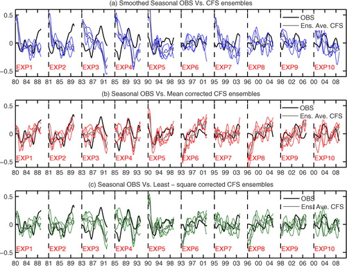
Figure 1a shows the PAA index calculated by using the annual SST anomalies predicted by the model and from the observations. During the first 2 yr, the simulated PAA index is warmer than in the observations. This is the case for the ensemble mean and most of the ensemble members. This systematic warm bias is effectively reduced when the CFS forecasts are corrected with the SMC and SLC methods, as shown in Fig. 1b and 1c, respectively. Similar results are noticed when the corrections are applied to the seasonal SST anomalies (Fig. 2). However, an apparent warming drift is manifested by the correction methods in experiments six and eight (Figs. 1 and 2). This unrealistic drift could be attributed to the smaller sampling of decadal forecasts which impose an apparent conditional nature on prediction skill as discussed by Goddard et al. (2013) and Meehl et al. (2013).

Fig. 1 Time evolution of the PAA index (°C) based on annual anomalies. (a) CFS ensembles in blue lines, (b) mean corrected in red and (c) least square corrected CFS ensembles in green lines. In all the panels, thick grey lines depict ensemble mean, and the black line corresponds to observations. X-axis shows the 10 initialised years with each initialised year separated by a vertical dashed line.

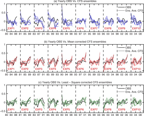
Fig. 2 Same as Fig. 1, but for seasonal anomalies.

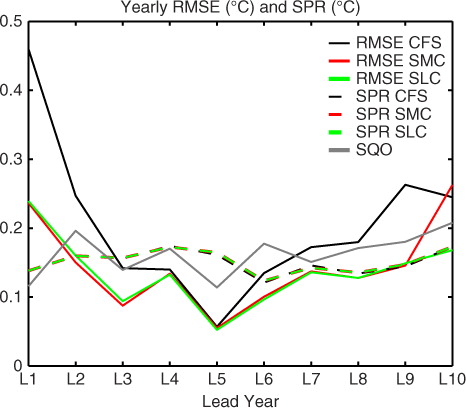
Figure 3 shows the RMSE of the annual forecasts and times standard deviation (referred as SQO hereafter) of the observations as a function of lead-time. The SQO indicates the limit of the saturation for error growth in RMSE beyond which the prediction skill is undetectable (Stan and Kirtman, 2008). The RMSE of the uncorrected annual PAA index is much higher than the SQO, especially during first 2 yr. This suggests that there is no decadal prediction skill detectable in the CFS forecasts. However, the SPR calculated for the CFS forecasts is lower than the SQO in the latter half of the decade, indicating that CFS model has decadal potential predictability at longer lead-times. Therefore, the lack of prediction skill of the CFS simulations may be due to the systematic biases in SSTs, which could explain the large values of the RMSE of the forecasts. The SMC and SLC methods demonstrate that the systematic biases indeed reduced the prediction skill of the CFS ensembles. In Fig. 3, the RMSE of the corrected forecasts using the SMC and SLC methods, respectively, are relatively lower than that of the uncorrected forecasts and become smaller than the SQO. Therefore, the correction methods systematically reduce the biases and increase the model prediction skill of annual anomalies on decadal timescales. The SPR, before and after employing the correction methods, is hardly changed because, in both correction methods, the correction term is estimated based on the ensemble mean state (Atger, 2003).

Fig. 3 Root mean square error (solid lines) and ensemble spread (dashed lines) of the PAA index (°C). The black line corresponds to the uncorrected forecasts, red line denotes the RMSE of the corrected forecasts using the SMC method and green line represents the RMSE of the corrected forecast using the SLC method. Note that the model spread is unchanged after the correction. The grey line depicts the times the standard deviation of the observations.

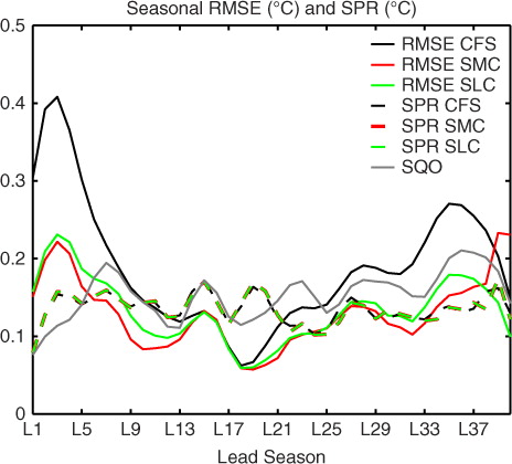
However, the RMSEs of the corrected PAA indices are still higher than the SQO of observations for the first year. This may simply be due to the differences between the SST ocean initial conditions used for the initialisation of the CFS forecasts, and the observed SSTs used in the validation. This feature is also present in the RMSEs of seasonal anomalies. Figure 4 is similar to Fig. 3, except that all the calculations are performed using seasonal anomalies. The RMSE and SPR on seasonal scales are very similar to that calculated using annual anomalies (compare Figs. 3 and 4).

Fig. 4 Similar to three, except the RMSEs and SPRs are calculated using seasonal anomalies.

The ACOR of annual anomalies is significantly improved after employing the correction methods (Fig. 5). A Monte-Carlo approach is used to check the statistical significance of the improvements noticed in the corrected forecasts. A sample of 10⁴ similar to CFS forecasts, but chosen from random numbers of normal distribution with zero mean and unit variance, are selected. All these samples are corrected with the SMC and SLC methods based on another similar random number sample chosen as observations. The ACOR is computed between each of the random 10⁴ samples and the random sample selected as observation before and after each of the bias-corrections is performed. The improvements in the ACOR at the 95th percentiles are captured for each of the correction method as difference between ACOR values before and correction at 95th percentile levels. These values represent 5% significant differences that are expected from performing correction on a random time-series. In our study, the ACORs computed with the SMC and SLC methods are examined to detect an improvement at any lead year beyond the corresponding 5% significant differences. This is achieved by examining whether the differences of ACOR for each of the SMC and SLC methods compared to uncorrected forecasts is higher than at least the corresponding 5% significant difference derived from Monte-Carlo approach. Note that the Monte-Carlo approach used here to identify the threshold for 5% significant ACOR values is different from a traditional t-test (Kim et al., 2012; Mochizuki et al., 2012).

Fig. 5 Anomaly correlations (solid line) of the uncorrected forecasts (black) and corrected forecasts (SMC method in red, and SLC method in green). The circles on the red and green solid lines show the 5% significant values of the correlation difference. The dashed lines show persistence forecasts for the uncorrected ensembles in black, SMC corrected in red, SLC corrected in green and the observations in grey lines. X-axis labels show the lead years. The grey horizontal line is drawn in the plot to highlight the transformation of negative to positive correlation after employing the bias corrections.

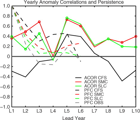
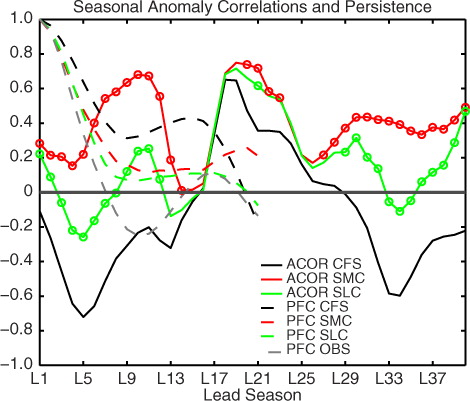
The persistence in the corrected forecasts is slightly reduced from that in the uncorrected forecasts (Fig. 5). The higher PFC of CFS forecasts partly explains the higher RMSE between CFS forecasts and observations. After correction, the persistence decreases more rapidly than in the uncorrected forecasts but the correlation values are still higher when compared to the observations. The ACOR and PFC analyses show that the correction methods significantly improved annual ACORs and adjusted the magnitude of PFC towards the observations. Similar significant improvements are also observed by bias-correcting the seasonal forecasts (Fig. 6).

Fig. 6 Similar to Fig. 5, but for seasonal anomalies.

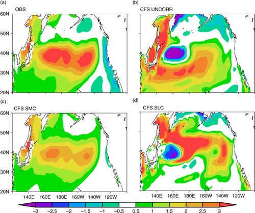
Regression of the SST anomaly forecasts in the PDV region on the corresponding PAA index reveals that SMC method produces a realistic covariability of SST anomalies with PAA index. Figure 7 shows the regression of seasonal SST anomaly forecasts on the corresponding PAA index averaged over all available cases. In the observations, there are two areas with positive coefficients from linear regression that are present in the west and the eastern half of the PDV region and negative coefficients are present along the American coast. The uncorrected forecasts are affected by errors in the form of large negative regression coefficients in the upper and weaker positive regression coefficients in the eastern half of PDV region (compare Fig. 7a and 7b). The SLC method diminishes the negative biases and also improves the weak-positive linear regression coefficients (Fig. 7d). The SMC method extensively reduces the erroneous negative correlation present in the uncorrected forecasts, and robustly improves the weak-positive coefficients from linear regression (Fig. 7c). The regression and correlation patterns (not shown) indicate that the spatial variability in the SST anomalies associated with the PAA index is improved with the SMC method compared to the SLC method. The spatial regression patterns suggest that the assumption of linear trend in the model drift as was assumed in the SLC method is not particularly suitable for correcting decadal predictions.

Fig. 7 Regression of SST anomalies on PAA (°C/°C) using (a) observations, (b) uncorrected forecasts, (c) SMC and (d) SLC methods.

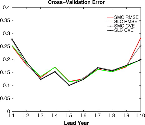
The robustness of the SMC and SLC methods is verified in cross-validation mode as follows. In each method, the correction term is estimated by removing one experiment out of the N _y available experiments, and this correction term is used to correct the bias in the experiment not included in the calculation of correction. After bias correcting each experiment this way, the RMSEs are computed against the observations and this represents the cross-validation error (CVE). Figure 8 shows the CVE as calculated for both correction methods along with the RMSEs. The RMSE and CVE values change very slightly in each of the correction methods suggesting the robustness of these bias correction methods. To test further whether the ensemble mean computed in eqs. (4) and (5) did not lead to overfitting the data (estimate higher parameters), the mean of N _y experiments is computed using various number of harmonics (H=1, 2, 3 and 4) as described in Narapusetty et al. (2009). Cross-validation procedure is repeated each time when the correction term [eqs. (4) and (5)] is computed using a different number of harmonics. The resulting CVE (not shown) revealed that the ensemble mean computed as a simple averaging did not lead to data over-fitting. Therefore, the simple averaging is not a problem in correcting the biases in annual anomalies of decadal forecasts. The similar conclusion is also reached when the cross validation technique is applied on seasonal anomalies (not shown). Though the robustness of the SMC and SLC methods examined in this study is satisfactory in terms of a cross-validation approach, the limited sampling size of the available ensembles poses uncertainty in the robustness of cross-validation (Gangstø et al., 2013).

Fig. 8 Red and green lines depict the RMSE as calculated using SMC and SLC methods, and grey and black lines represent the cross validation error (CVE) for SMC and SLC methods, respectively.

Figure 9 shows the reliability diagrams of CFS and corrected forecasts for lead years one, two, six and eight. In this reliability diagram, the condition for the forecast probability versus observation frequency is that SST anomalies in the individual forecasts are higher than half of the standard deviation of the CFS ensembles. Concurrently, matching observations are higher than half of the standard deviation of observations. This scenario diagnoses model's ability to capture the warmer events. The grey diagonal line in all the panels indicates that model forecasts reproduce the event at the same frequency as it occurs in the observations and should be considered as a reference for perfect reliability. The reliability diagram depicts the curve for the probability bins selected at 0.0, 0.25, 0.5, 0.75 and 1.0. Curves above the perfect reliability line indicate that the model under-predicts the event, whereas curves located below denote that the model gives false alarms by reproducing the event with high probability. Generally, a flat reliability curve compared to the ideal-scenario grey line, indicates over-confident and consistently false-alarmed nature of forecasts (Barnston et al., 2003). The number of events that fall in the probability bins 0.0, 0.25, 0.5, 0.75 and 1.0 are shown in histograms (Fig. 9). The number of events falling in the bins of histogram reveals the sampling size of the statistic in study. The reliability curves in conjunction with the histograms reveal distribution of probabilities of the event to occur.

Fig. 9 The black, red and green lines in left column of panels show the forecast reliabilities for the uncorrected, SMC and SLC-corrected forecasts, respectively, in lead years (a) one, (b) two, (c) six and (d) eight. The condition for the forecast probabilities is described in the text. In all the panels, the grey diagonal line corresponds to the ideal scenario for perfect reliability. The three histograms identified with corresponding colours, placed next to each panel show the number of forecast events (in that particular lead year) organised in probability bins of 0, 0.25, 0.5, 0.75 and 1.0 shown with bin numbers 1–5, respectively.

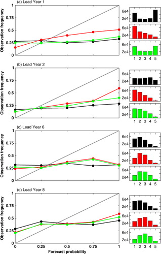
The reliability diagrams of the warm events in the first and second lead years (Fig. 9a and 9b) show an improvement in the probabilistic skill of the corrected forecasts. The reliability diagrams shown in Fig. 9c and 9d for the six and eight lead years, respectively, underscore the improvements in the forecast probability at longer lead-times in the bias corrected forecasts. The similar improvements are also examined in the other years (not shown). In all the lead years, the reliability curves of the uncorrected forecasts are flatter compared to the SMC and SLC derived forecasts. This indicates that CFS produces forecasts with longer persistence, which is consistent with the PFC analysis (see Fig. 5). The reliability diagrams for cold events (not shown) also reveal that the bias correction methods slightly improve the reliability of the probabilistic forecast skill. The reliability of SMC derived forecasts is similar to the SLC derived forecasts in the first lead year, however, for the later lead years, the former is slightly better than the latter (e.g. Fig. 9b, 9c and 9d). The histograms reported in each lead year (Fig. 9) indicate sufficiently larger sampling of events across the probability bins.

The higher number of warmer events as recorded in the histograms of uncorrected forecasts during the first 2 yr (in Fig. 9a and 9b) are related to the uncorrected forecast's warm-bias in the first few years in most of the experiments (Fig. 1a). In years 6 and 8, the number of warm events of high probability bin in the histograms is reduced (Fig. 9c and 9d) due to the consistency in occurrence of colder events among the forecast ensembles (Fig. 1). The lack of sharpness in the histograms, in particular lesser events recorded in the bin that indicate probability one (Fig. 9b, 9c and 9d) indicates the higher ensemble spread with respect to observations. The sharpness of histograms did not improve with the correction, as the model spread is very similar among corrected and uncorrected forecasts (Fig. 3). However, for each of uncorrected, SMC and SLC forecasts, a larger number of samples are included in each probability bin of histograms, therefore, the lack of sharpness does not affect the conclusions of reliability.

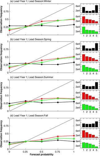
Annual anomalies generally consider only the low-frequency part of the variability, and the reliability of the extreme annual forecasts obtained by applying the forecast reliability techniques may not necessarily be extrapolated to the reliability of the seasonal forecast predictions of the model. To understand the relationship between the reliabilities of seasonal and annual forecasts, the reliability diagrams for individual seasons are also examined. Figure 10 shows the reliability diagrams for seasonal forecasts simulating the warm events in the observations for the lead year 1. The bias correction methods improved the reliability in the winter and spring seasons compared to the other two seasons. Examining the forecast reliability in capturing cold events also revealed that bias corrected methods improve the forecast reliability of the winter and spring forecasts compared to summer and fall forecasts (not shown). At the longer lead-seasons (beyond a year), SMC derived forecasts have a slightly higher reliability than the SLC derived forecasts consistent with the conclusions derived based on Fig. 9b, 9c and 9d. Note that the CFS data utilised in this study does not follow the initialised states of CMIP-5 protocol (1960–2005 initialised with 5 yr apart), but, the applications shown here are universal to the decadal forecasts with the caveats of model dependency. In this study, we analysed bias correction methods for SSTs in the Northern Pacific; however, these methods are also applicable to SSTs in the other regions as well as for any other variable.

Fig. 10 Similar to Fig. 9, but the forecast reliability shown in (a) winter (DJF), (b) spring (MAM), (c) summer (JJA) and (d) fall (SON) of the first lead year.

4. Conclusions

The main goal of this study is to understand to what extent bias correction methods can improve the decadal forecast skill. Decadal hindcasts/forecasts represent a new type of numerical experiment in an attempt to extend the existing forecasting capabilities to decadal timescales. Toward that goal, a SMC and a least-square bias correction method are explored for the possible reduction of the impact of model systematic errors in forecasting the north Pacific SST variability. The forecasts are produced by the Climate Forecasting System version 2, a state-of-the-art forecast system. The two correction methods used in this study are routinely used to reduce biases in short-term weather forecasts. The improvement in the prediction skill of forecasting north Pacific SST anomalies is evaluated with both deterministic and probabilistic diagnostics.

The results show that the bias corrected methods significantly reduce the RMSEs of seasonal and annual north Pacific SST forecasts, and thereby improve the forecast skill of PAA index that is constructed as the spatial average of SST anomalies over 20°–60°N and 120°E–100°W. The bias corrected forecasts show significant improvements for most of the lead-times in the ACOR diagnostic. However, a Monte-Carlo significance test reveals that annual bias corrected forecasts show improvements that are statistically significant at the 5% level in forecasts for longer lead-time than do the seasonally averaged forecasts. This result suggests that both the annual and seasonal forecasts do benefit from the bias correction methods in terms of forecasts skill. The uncorrected CFS forecasts exhibit stronger persistence compared to observations indicating the existence of model systematic bias. Our results also indicate that this persistence is reduced with bias correction methods. The regression analysis and correlation between SST anomalies and corresponding PAA index in the PDV region show much improved spatial patterns in the bias corrected forecasts.

The reliability in forecasting warmer and colder SSTs is also improved with the bias correction. The reliability diagrams reveal that, compared to the uncorrected forecasts, the bias-corrected seasonally and annual SST anomaly forecasts are more reliable in capturing both warm and cold extreme events up to eight of the 10 forecasted years. Reliability diagrams also suggest that the bias corrected winter and spring seasonal forecasts contribute more to the forecast reliability than do summer and fall forecasts.

The comparison between SMC and SLC bias correction methods indicates that the forecast skill of the SMC derived SST anomalies is slightly better than that of the SLC method. The SMC derived SST anomalies also reproduce extreme events more reliably. The regression and correlation patterns (not shown) indicate that the SMC method reproduces the spatial pattern in the SST anomalies associated with the PAA index compared to the SLC method.

The correction methodology in this study assumes that, in all the CFS decadal forecasts, the SST variability due to the external forcing is consistent with observations, therefore, the external forcing is not a source of uncertainty. This is a reasonable assumption given the short span of the initial states of the forecasts discussed in this study. However, if the forecasts to be corrected cover periods with different external forcing it is required to perform a trend correction (Kharin et al., 2012) before applying the bias-correction techniques discussed in this study.

This study is aimed at improving the decadal forecast skills by correcting model systematic biases. Therefore, the improvements in the decadal forecast skill demonstrated with the bias correction methods are applicable to correct the systematic biases of the CMIP5 participating model forecasts.

5. Acknowledgements

This research was funded by NOAA grant NA09OAR4310137. We gratefully acknowledge National Centers for Environmental Prediction (NCEP) for the CFS v2 model made available to COLA. We also acknowledge S. Saha of EMC/NCEP/NWS/NOAA for making the CFS v2 forecasts available to us. We thank Dr. Tim DelSole of GMU/COLA for helpful discussions. We particularly wish to thank W. Lapenta and L. Uccellini for enabling the collaborative activities.

References

- Atger F . Spatial and interannual variability of the reliability of ensemble-based probabilistic forecasts: consequences for calibration. Mon. Weather Rev. 2003; 131: 1509–1523. DOI: 10.1175//1520-0493(2003)131<1509.
- Barnston A. G. , Mason S. J. , Goddard L. , DeWitt D. G. , Zebiak S. E . Multimodel ensembling in seasonal climate forecasting at IRI. Bull. Am. Meteorol. Soc. 2003; 84: 1783–1796. DOI: 10.1175/BAMS-84-12-1783.
- Branstator G. , Teng H . Two limits of initial-value decadal predictability in a CGCM. J. Clim. 2010; 23: 6292–6311. DOI: 10.1175/2010JCLI3678.1.
- Branstator G. , Teng H. , Meehl G. A. , Knight J. R. , Latif M. , co-authors . Systematic estimates of the initial-value decadal predictability for six AOGCMs. J. Clim. 2012; 25: 1827–1846. DOI: 10.1175/JCLI-D-11-00227.1.
- Buizza R . Potential forecast skill of ensemble prediction and spread and skill distributions of the ECMWF ensemble prediction system. Mon. Weather Rev. 1997; 125: 99–119. DOI: 10.1175/1520-0493(1997)125<0099.
- Chikamoto Y. , Kimoto M. , Ishii M. , Mochizuki T. , Sakamoto T. , co-authors . An overview of decadal climate predictability in a multi-model ensemble by climate model MIROC. Clim. Dyn. 2012; 30: 1201–1222. DOI: 10.1007/s00382-012-1351-y.
- Corti S. , Weisheimer A. , Palmer T. , Doblas-Reyes F. , Magnusson L . Reliability of decadal predictions. Geophys. Res. Lett. 2012; 39: L21712. DOI: 10.1029/2012GL053354.
- Deser C. , Alexander M. , Xie S. P. , Phillips A . Sea surface temperature variability: patterns and mechanisms. Ann. Rev. Mar. Sci. 2010; 2: 115–143. DOI: 10.1146/annurev-marine-120408-151453.
- Deser C. , Phillips A. S. , Hurrell J. W . Pacific interdecadal climate variability: linkages between the tropics and the north pacific during boreal winter since 1900. J. Clim. 2004; 17: 3109–3124. DOI: 10.1175/1520-0442(2004)017<3109.
- Doblas-Reyes F. J. , Balmaseda M. A. , Weisheimer A. , Palmer T. N . Decadal climate prediction with the European center for medium-range weather forecasts coupled forecast system: impact of ocean observations. J. Geophys. Res. 2011; 116: 19111. DOI: 10.1029/2010JD015394.
- Dosio A. , Paruolo P . Bias correction of the ensembles high-resolution climate change projections for use by impact models: Evaluation on the present climate. J. Geophys. Res. 2011; 116: D16106. DOI: 10.1029/2011JD015934.
- Feudale L. , Tompkins A. M . A simple bias correction technique for modeled monsoon precipitation applied to west Africa. Geophys. Res. Lett. 2011; 38: L03803. DOI: 10.1029/2010GL045909.
- Gangstø R. , Weigel A. P. , Liniger M. A. , Appenzeller C . Methodological aspects of the validation of decadal predictions. Clim. Res. 2013; 55: 181–200. DOI: 10.3354/cr01135.
- Ge Y. , Gong G . North American snow depth and climate teleconnection patterns. J. Clim. 2009; 22: 217–233. DOI: 10.1175/2008JCLI2124.1.
- Goddard L. , Kumar A. , Solomon A. , Smith D. , Boer G. , co-authors . A verification framework for interannual-to-decadal predictions experiments. Clim. Dyn. 2013; 40: 245–272. DOI: 10.1007/s00382-012-1481-2.
- Guemas V. , Corti S. , Garcia-Serrano J. , Doblas-Reyes F. J. , Balmaseda M. , co-authors . The Indian ocean: the region of highest skill worldwide in decadal climate prediction. J. Clim. 2013; 26: 726–739. DOI: 10.1175/JCLI-D-12-00049.1.
- Gupta A. S. , Muir L. C. , Brown J. N. , Phipps S. J. , Durack P. J. , co-authors . Climate drift in the CMIP3 models. J. Clim. 2012; 25: 4621–4639. DOI: 10.1175/JCLI-D-11-00312.1.
- Hegerl G. C. , Zwiers F. W. , Braconnot P. , Gillett N. P. , Luo Y. , co-authors . Hegerl G. C. , etal. Understanding and attributing climate change. Climate Change 2007: The Physical Science Basis. 2007; 663–745. Contribution of working group I to the fourth assessment report of the Intergovernmental Panel on Climate Change. Cambridge University Press, Cambridge.
- ICPO (International CLIAVR Project Office). Data and bias correction for decadal climate predictions. World Clim. Res. Prog. Rep. 2011; 150: 1–3.
- John V. O. , Soden B. J . Temperature and humidity biases in global climate models and their impact on climate feedbacks. Geophys. Res. Lett. 2007; 34: L18704. DOI: 10.1029/2007GL030429.
- Katz S. L. , Hampton S. E. , Izmest'eva L. R. , Moore M. V . Influence of long-distance climate teleconnection on seasonality of water temperature in the world's largest lake—Lake Baikal, Siberia. PLoS One. 2011; 6: e14688. DOI: 10.1371/journal.pone.0014688.
- Kharin V. V. , Boer G. J. , Merryfield W. J. , Scinocca J. F. , Lee W. S . Statistical adjustment of decadal predictions in a changing climate. Geophys. Res. Lett. 2012; 39: L19705. DOI: 10.1029/2012GL052647.
- Kim H. , Webster P. J. , Curry J. A . Evaluation of short-term climate change prediction in multi-model CMIP5 decadal hindcasts. Geophys. Res. Lett. 2012; 39: L10701. DOI: 10.1029/2012GL051644.
- Kumar A. , Barnston A. G. , Hoerling M. P . Seasonal predictions, probabilistic verifications, and ensemble size. J. Clim. 2001; 14: 1671–1676. DOI: 10.1175/1520-0442(2001)014<1671.
- Large W. G. , Danabasoglu G . Attribution and impacts of upper-ocean biases in CCSM3. J. Clim. 2006; 19: 2325–2346. DOI: 10.1175/JCLI3740.1.
- Mechoso C. R. , Robertson A. W. , Barth N. , Davey M. K. , Delecluse P. , co-authors . The seasonal cycle over the tropical pacific in coupled ocean–atmosphere general circulation models. Mon. Weather Rev. 1995; 123: 2825–2838. DOI: 10.1175/1520-0493(1995)123<2825.
- Meehl G. A. , Stocker T. F. , Collins W. D. , Friedlingstein P. , Gaye A. T. , co-authors . Global climate projections. Climate Change 2007: The Physical Science Basis (eds. Solomon, S., D. Qin, M. Manning, Z. Chen, M. Marquis, K. B. Averyt, M. Tignor and H. L. Miller) . 2007; 747–845. Contribution of working group I to the fourth assessment report of the intergovernmental panel on climate change. Cambridge University Press, Cambridge.
- Meehl G. A. , Goddard L. , Murphy J. , Stouffer R. J. , Boer G. , co-authors . Decadal prediction can it be skillful?. Bull. Am. Meteorol. Soc. 2009; 1467–1485. DOI: 10.1175/2009BAMS2778.1.
- Meehl G. A. , Goddard L. , Boer G. , Burgman R. , Branstator G. , co-authors . Decadal climate prediction: an update from the trenches. Bull. Am. Meteorol. Soc. 2013; 1467–1485. early online release DOI: 10.1175/BAMS-D-12-00241.1.
- Mochizuki T. , Chikamoto T. , Kimoto M. , Ishii M. , Tatebe H. , co-authors . Decadal prediction using a recent series of miroc global climate models. J. Meteorol. Soc. Jpn. 2012; 90A: 373–383. DOI: 10.2151/jmsj.2012-A22.
- Mochizuki T. , Ishii M. , Kimoto M. , Chikamoto Y. , Watanabe M. , co-authors . Pacific decadal oscillation hindcasts relevant to near-term climate prediction. Proc. Natl. Acad. Sci. U. S. A. 2009; 107: 1833–1837. DOI: 10.1073/pnas.0906531107.
- Narapusetty B. , DelSole T. , Tippett M. K . Optimal estimation of the climatological mean. J. Clim. 2009; 22: 4845–4859. DOI: 10.1175/2009JCLI2944.1.
- Power S. , Casey T. , Folland C. , Colman A. , Mehta V . Interdecadal modulation of the impact of ENSO on Australia. Clim. Dyn. 1999; 15: 319–324. DOI: 10.1007/s003820050284.
- Richardson D. S . Ensembles using multiple models and analyses. Q. J. Roy. Meteorol. Soc. 2001; 127: 1847–1864. DOI: 10.1002/qj.49712757519.
- Saha S. , Nadiga S. , Thiaw C. , Wang J. , Wang W. , co-authors . The NCEP climate forecast system. J. Clim. 2006; 19: 3483–3517. DOI: 10.1175/JCLI3812.1.
- Saha S. , Nadiga S. , Thiaw C. , Wang J. , Wang W. , co-authors . The NCEP climate forecast system reanalysis. Bull. Am. Meteorol. Soc. 2010; 91: 1051–1057. DOI: 10.1175/2010BAMS3001.1.
- Saha S., Moorthi S., Wu X., Wang J., Nadiga S., co-authors. The NCEP climate forecast system version 2. J. Clim. 2013. DOI: http://dx.doi.org/10.1175/JCLI-D-12-00823.1. early online release.
- Smith T. M. , Reynolds R. W. , Peterson T. C. , Lawrimore J . Improvements to NOAA's historical merged land–ocean surface temperature analysis. J. Clim. 2008; 21: 2283–2296. DOI: 10.1175/2007JCLI2100.1.
- Stan C. , Kirtman B. P . The influence of atmospheric noise and uncertainty in ocean initial conditions on the limit of the predictability in a coupled GCM. J. Clim. 2008; 21: 3487–3503. DOI: 10.1175/2007JCL2071.1.
- Stockdale T. N . Coupled ocean–atmosphere forecasts in the presence of climate drift. Mon. Weather Rev. 1997; 125: 809–818. DOI: 10.1175/1520-0493(1997)125<0809.
- Trenberth K. E. , Hurrell J. W . Decadal atmosphere–ocean variations in the Pacific. Clim. Dyn. 1994; 9: 303–319. DOI: 10.1007/BF00204745.
- Van-Oldenborgh G. J. , Doblas-Reyes F. J. , Wouters B. , Hazeleger W . Decadal prediction skill in a multi-model ensemble. Clim. Dyn. 2012; 38: 1263–1280. DOI: 10.1007/s00382-012-1313-4.
- von Storch H. , Zwiers F. W . Statistical Analysis in Climate Research. 1999; 484. Cambridge University Press, Cambridge, United Kingdom.
- Wilks D. S . Statistical Methods in the Atmospheric Sciences. 1995; San Diego: Academic Press. 467.
- Yeager S. , Karspeck A. , Danabasoglu G. , Tribbia J. , Teng H . A decadal prediction case study: late twentieth-century North Atlantic ocean heat content. J. Clim. 2012; 25: 5173–5189. DOI: 10.1175/JCLI-D-11-00595.1.