Mass exchange at the Strait of Gibraltar in response to tidal and lower frequency forcing as simulated by a Mediterranean Sea model

Abstract

The exchange between the Atlantic and the Mediterranean at the Strait of Gibraltar is studied based on numerical simulations of the Mediterranean Sea compared to two sets of observations. The model used has a varying horizontal resolution, highest at the Strait of Gibraltar. Numerical simulations forced by tide, by the subinertial variability, by both and by increasing the diffusion at the Strait are performed and compared to each other. The model successfully reproduces the main observed features of the variability at the tidal and at the lower frequency time scales including the phasing between the barotropic and baroclinic flow components and density variations. The model also simulates the strong mixing at the strait by tide and the resulting fortnightly modulation of the flow, with exchange reduction during spring tides and outflowing waters and acceleration during neap tides and inflowing waters. It is shown that tidal oscillations reduce the two-way exchange by interaction with the subinertial variability. The effects of tide on the Mediterranean Sea thermohaline circulation are also examined using multi-decadal simulations. It is shown that the model reproduces the cooling and saltening of waters crossing the strait in the upper layer and the warming and freshening of waters crossing the strait in the deeper layer, as previously shown by high resolution models of the Strait of Gibraltar. These changes are shown to cool and increase the salinity of the Mediterranean waters especially in the upper and intermediate layers. The water-cooling is shown to lead to a reduction of the heat loss at the sea surface. Based on model results, it is concluded that tide may have an effect on the Mediterranean Sea heat budget and hence on the atmosphere above. A validation of this conclusion is however needed, in particular using higher resolution models.

• Strait of Gibraltar
• Mediterranean Sean
• tide
• thermohaline circulation
• water flow
• hydrographic changes

1. Introduction

The Strait of Gibraltar is a very energetic area of the sole pathway between the Mediterranean Basin and the Atlantic Ocean (Lacombe and Richez, 1984; Armi and Farmer, 1988). The two-way exchange is very intense. Each flow is nearly 20 times larger than the net water lost at the sea surface. The intense hydrographic changes incurred by the surface Mediterranean waters due to the strong evaporation explain the existence of the basin wide circulation cell that extends westward into the Atlantic. At the Strait of Gibraltar, the upper and lower branches of this cell form the two layers of the exchange. The exchange exhibits a weak seasonal cycle (García Lafuente et al., 2002a) but the variability is mostly subinertial, generated by the atmospheric variability at the Mediterranean Sea surface (mainly the atmospheric pressure fluctuations, Candela et al., 1989, 1990; Candela, 1991) with some contribution of wind stress (García Lafuente et al., 2002b). Tide is also an important forcing of the flow at Gibraltar. Tidal oscillations, mainly semi-diurnal, induce large water fluxes that reach 5 Sv during spring tides. Flow fluctuations induced by tide and by the subinertial variability are mainly barotropic but a baroclinic component exists (Candela et al., 1989). This component is linked to interactions between tide and the subinertial variability (Vargas et al., 2006). The Strait topography induces highly complex flow structures. The shallow Camarinal sill and the Tangier basin west of it create dynamical conditions favourable for supercritical flows, hydraulic jumps, bores and wave release.

Candela et al. (1989) first revealed the baroclinic fortnightly variability of the flow at the Strait of Gibraltar exhibiting a decrease of the velocity shear during spring tides and an increase during neap tides. The fortnightly signal was also shown by García Lafuente et al. (2013) who found that the interface is thicker during spring tides and Vargas et al. (2006) who showed that the shear is reduced during spring tides with the interface sinking and the opposite during neap tides. The authors showed a fortnightly variability in the lower layer transport with a maximum outflow during spring tides. They also showed that transports based on the low-frequency variability (periods larger than tidal ones) and high frequency oscillations (related to interface vertical movements) cancel in the upper layer but not in the lower layer explaining the fortnightly variability found only in the lower layer. The baroclinic component is explained as resulting from tidal mixing in the sill that accounts only for the fortnightly variability of the lower layer transport. The baroclinic fortnightly variability is also suggested to result from a dynamical balance between the water masses transported by barotropic tide fluctuations, that generate water exchange and mixing, and those transported by baroclinic fluctuations (Harzallah, 2009).

The shallow Camarinall sill in the western side of the Strait strongly influences the dynamics of the exchange. The sill blocks the water crossing the Strait towards the Atlantic (Sánchez-Román et al., 2012) leading to an interface rise. The release of waters leads to a hydraulic jump and generates internal waves that propagate eastward. In addition, large mixing occurs in the shallow area west of the Camarinal sill (the Tangier Basin). The resulting mixed waters progress eastward after their release (Armi and Farmer, 1988; Macias et al., 2006; Sánchez-Román et al., 2012; García Lafuente et al., 2013). These last authors showed that the eastward advection of the mixed waters west of the Camarinall Sill, the entrainment further east and the friction inside the mixed layer all contribute to the dynamics of the interface layer. The generated waves are found to reach the Bay of Algeciras where they are suggested to lead to notable vertical mixing (Chioua et al., 2013). The wave formation is influenced by the subinertial variability (Vázquez et al., 2008). It is inhibited by the mean water inflow (resulting from low atmospheric pressure over the Mediterranean) even during spring tides. At the opposite, the mean water outflow (due to high atmospheric pressure) may activate waves even during neap tides.

Several numerical models were developed to simulate the tide propagation through the Strait of Gibraltar. Examples of such models are those of Dressler (1980) using 1/3° as resolution, Vincent and Canceill (1993) using 10 to 20 km as resolution with assimilation of tide in some points and Sanchez et al. (1992) using 1/2° as resolution. Tsimplis et al. (1995) used a 2D model (1/12° as resolution) to simulate the tide propagation in the Mediterranean Sea and showed that both tide coming from the Atlantic and the equilibrium tide are important in the Mediterranean basin but the former is dominant close to the Strait. For the M2 component they showed that the contribution of the equilibrium tide is weak west of 1°E. Wang (1989) developed a 3D model of tide at the Strait of Gibraltar which reproduced most of the observed features. Sannino et al. (2004) used a model for the semidiurnal (M2 and S2) tide components at the Strait of Gibraltar based on the model implemented for the mean flow at the Strait by Sannino et al. (2002). The model results were in good agreement with the observed tidal elevation amplitudes and phases; the semidiurnal tide increases water inflow and outflow by 30%. Using a very high-resolution model of the Strait of Gibraltar, Sánchez-Garrido et al. (2011) obtained complex baroclinic structures created as a response to the barotropic tide in the Camarinal Sill. These structures are found dependent on the amplitude of the tide.

Recently some modelling studies examined the long-term evolution of the Mediterranean Sea in relation with the exchange at the Strait of Gibraltar. Fenoglio-Marc et al. (2013) showed an increase in the net water flux at Gibraltar during the period 1970–2009 derived by the decadal variability of the net evaporation at the sea surface. They showed that Mediterranean mass changes are comparatively small with no long-term trend. Based on a 80-yr long simulation, Sannino et al. (2009) showed that model grid refinement at the Strait of Gibraltar leads to a better representation of the flow in the Strait and to a better representation of water column stratification in the Mediterranean basin and consequently on the characteristics of the convection events as was the case in the Gulf of Lions.

This paper investigates the barotropic and baroclinic components of the flow through the Strait of Gibraltar and their variability related to tidal oscillations and to the lower frequency subinertial forcing. The impacts of tidal oscillations on the Mediterranean basin waters are also examined. The paper compares results from a Mediterranean Sea model to observations inside the Strait analysed and presented in previous work (e.g. Harzallah, 2009). The next section of the paper presents the model and the data used. Section 3 presents the simulated tide at the Strait of Gibraltar. Section 4 analyses the amplitude and phase of tide and of the low frequency oscillations in the Strait from model simulations and from observations. Section 5 shows the simulated mass transport at the Strait of Gibraltar. Section 6 presents the effects of the use of tide as a model forcing on the thermohaline circulation of the Mediterranean Sea. The paper ends with some conclusions.

2. Model and data used

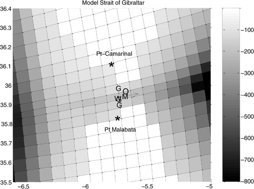
INSTMED06 (Alioua and Harzallah, 2008) is a 3D hydrodynamical model of the Mediterranean Sea based on the Princeton Ocean Model (Mellor and Yamada, 1982; Mellor and Blumberg, 1985; Mellor, 1996). It was used to study long-term changes in the Mediterranean Sea (Gualdi et al., 2013). The model bathymetry is from the ETOPO5 (5′X5′ resolution) database (Smith and Sandwell, 1997). The bathymetry is slightly smoothed to reduce the hydrostatic inconsistency with sigma coordinates (Haney, 1991; Mellor et al., 1994). The resulting bathymetry (Fig. 1) reasonably reproduces the main sub-basins and straits of the Mediterranean Sea. The depth reaches 3000 to 4000 m in the Levantine basin, and nearly 2700 in the central western basin and the Tyrrhenian Sea. The smoothing of the Strait of Sicily is relatively high with one sill at 1380 m depth. At the Strait of Gibraltar the model bathymetry is characterised by a 230 m depth sill located at 5.8°W (the Camarinal Sill) and a 230 m depth secondary sill located at 6.1°W (Fig. 2). The bathymetry deepens rather rapidly at the western entrance of the Strait.

Fig. 1 Bathymetry used for the INSTMED06 Mediterranean Basin model. OTIS sea-level height tidal predictions used to force the INSTEMD06 are located at the first longitudinal grid point (7.9°W; 35.83°N) indicated by the ‘*’ sign.

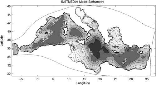
Fig. 2 Detailed bathymetry shown in Fig. 1 for the Strait of Gibraltar. The model grid is also plotted. The model has three grid points at the narrowest north–south section of the Strait. The locations of GE (velocity, temperature and salinity) and WOCE (velocity) measurements are shown by ‘G’ and ‘W’ letters, respectively; the location of tide currents from OTIS predictions is shown by the ‘O’ letter. The ‘M’ letter indicates the model grid point where the simulated temperatures and salinity are diagnosed. The arrow indicates the location where the simulated velocity is diagnosed. Density is derived at location ‘G’ for GE observations and ‘M’ for the model. The simulated volume transport through the Strait is calculated at the section crossed by the arrow.

The model calculates the three components of the velocity, the potential temperature and salinity. The model has 27 layers on the sigma coordinate. Horizontally the grid is curvilinear. The grid covers the whole Mediterranean Sea and extends westward over the Atlantic Ocean to nearly 7.8°W (a buffer zone). The domain does not include the Black Sea. The resolution is of 1/6°, but it is strongly increased at the Strait of Gibraltar where the minimum width is represented by three grid points (Fig. 2). At this section the latitudinal grid distance is ~4 Km. The model takes into account water input from rivers (Vorosmarty et al., 1998) as monthly climatology values. It uses a free sea surface forced by the atmospheric pressure and by water and heat fluxes. The water temperature and salinity at the sea surface are relaxed towards the observed climatology values (Brasseur et al., 1996; Brankart and Pinardi, 2001) with a time scale of 5 d. These data sets are also used to construct initial conditions for a 30-yr spin-up simulation and boundary conditions in the Atlantic buffer zone. A constant inflow from the Black Sea is considered but water mass, heat and salt exchanges are calculated by the model considering the temperature and salinity climatology at the Bosphorus Strait. At the western limit of the Atlantic buffer zone the model uses open boundary conditions. A radiation condition is applied to the sea level whereas simple inflow conditions are applied to the barotropic and baroclinic components of the horizontal velocity. Hence the model calculates the water velocity at the western limit given the sea-level at this location. There is no ‘instantaneous equilibrium condition’ that equilibrates the water loss at the surface to the input through the Strait of Gibraltar. Tide is taken into account by adding to the western boundary sea level height, the tide height increment. Temperature and salinity in the buffer zone are relaxed toward the climatology with a time scale ranging from 3 d at the western boundary to 100 d close to the Strait of Gibraltar. The model does not use the Boussinesq approximation in the current study.

The atmospheric forcing is model-downscaled reanalysis. It is generated by the LMDZ-Mediterranean model, a global atmospheric general circulation model with variable grid (Li, 1999; Hourdin et al., 2006) zoomed over the Mediterranean Sea (L'Hévéder et al., 2013; Rojas et al., 2013). The resolution is increased to 30 Km in the Mediterranean area. The atmospheric model is nudged outside the Mediterranean domain to the ERA reanalysis (Dee et al., 2011). The resulting surface downscaled fluxes for the 50-yr period 1958–2007 are used to force the INSTMED06 model. Daily forcing fields are used in the present work but at each model time step (10 mn with 20 s for the barotropic mode) instantaneous values are obtained by linear interpolation. As mentioned earlier a 30-yr spin-up simulation is first performed using three loops of repeated decade forcing, 1958–1967.

The data used for exchanges at the Strait of Gibraltar are from three sources. The first two, labelled GE and WOCE, were already used in Harzallah (2009). GE (Gibraltar Experiment, October, 1985–October, 1986; Pillsbury et al., 1987; Candela et al., 1989; Bryden et al., 1994; Wesson and Gregg, 1994; Morozov et al., 2002) are current meters measurements moored along a section laying close to the Point Malabata-Point Camarinal transect (nearly 5.74′W) in the Camarinal Sill (Fig. 2). WOCE (Word Ocean Circulation Experiment, almost 2 yr, November, 1994–September, 1996; Astraldi et al., 1999; Candela, 2001) has measurements using Doppler currents profiles (ADCPs) at a single point located almost on the same section (see Fig. 2). GE and WOCE data were processed in Harzallah (2009) to hourly series of along-strait velocity component, (and of temperature and salinity for GE) with drift corrected. Vertical profiles and transports were presented in Harzallah (2009). The period considered is from October 22, 1985 at 16:00 to April 21, 1986 at 07:00 for GE. For WOCE the first subset of the measurements corresponding to the period from November 8, 1994 at 17:00 to April 3, 1995 at 17:00 is considered (hereafter referred to as WOCE1). It should be mentioned that other data sets are available as the ADCP measurements in the Espartel Sill west of the Strait. This data lasted from September 2004 to September 2007 (Sánchez-Román et al., 2008, 2009) and in the East of the Strait from May to June 2003. A table summarising the measurements at the Strait is given by (Sánchez-Román et al., 2009). Due to model's low resolution, all data sets used represent the mean exchange at the Strait of Gibraltar without considering the along-strait and cross-strait spatial variability within the Strait.

For tide forcing, the Oregon State University Tidal Inversion Software (OTIS, Egbert et al., 1994; Egbert and Erofeeva 2002) predictions are used. Arabelos et al. (2007) compared three different tide models in the Mediterranean Sea including OTIS one. They found that the three models are in a good agreement. OTIS tide was successfully used by Sánchez-Román et al. (2009) in a high-resolution tide model covering the Strait of Gibraltar. Arabelos et al. (2010) also used OTIS in a tide model of the Mediterranean Sea. The OTIS predictions consider the eight leading tidal components (M2, S2, N2, K2, K1, O1, P1 and Q1). Minor components are not included in this study since their contributions are very weak. In the present work, sea level variations induced by tide are predicted at the location (7.9°W; 35.83°N, see Fig. 1). Prior to the simulation, the tide coefficients for the eight modes are calculated following OTIS. During the simulation, the model calculates at each time step the total tide height based on the tide coefficients. As the Atlantic buffer zone of the model covers a rather small area, the same predicted elevation at (7.9°W; 35.83°N) is set for all western boundary grid points. Using the tidal forcing, the model dynamics provides the tide flow at the Strait.

Simulations performed with the INSTMED06 model are summarised in Table 1. The first simulation (STIW1) uses the predicted sea-level height tidal oscillations as a forcing, as detailed above. The simulation covers the WOCE1 observation sub-period, November 8, 1994 at 17:00 to April 3, 1995 at 08:00. The simulation is started well in advance (January 1, 1994) to ensure the spin-up of the model with tide forcing. A similar early starting is applied for all simulations where tide is included. The analysed model velocity at the Strait of Gibraltar corresponds to the location shown in Fig. 2. The second simulation (SNTW1) is similar to the first one but without tide. The third simulation (STAW1) uses the tide as forcing but all daily atmospheric fields are kept constant, the same as those at the starting of the simulation. This simulation is devoted to investigate directly the role of tides without any variation in atmospheric forcing. Similar to STIW1, a simulation (STIGE) is performed with the GE period tide forcing: October 22, 1985 at 16:00 to April 21, 1986 at 07:00. This simulation permits to compare in addition to the flow, the density characteristics derived from the model and from observations.

Table 1. Summary of datasets used and simulations performed

Acronym	Type	Period covered	Characteristics
GE	Data	October 22, 1985 at 16:00 to April 21, 1986 at 07:00	Along-strait water velocity and water density
WOCE1	Data	November 8, 1994 at 17:00 to April 3, 1995 at 17:00	Along-strait water velocity
STIGE	Simulation with tide	January 1, 1985 at 00:00 to April 21, 1986 at 07:00	Varying atmospheric forcing Tide forcing
SNTW1	Simulation without tide	January 1, 1994 at 17:00 to April 3, 1995 at 08:00.	Varying atmospheric forcing No tide forcing
STIW1	Simulation with tide	Varying atmospheric forcing Tide forcing
STAW1	Simulation with tide alone	Constant atmospheric forcing Tide forcing
SNT50	Long simulation without tide	50-yr: 1958–1967	Varying atmospheric forcing No tide forcing
STI50	Long simulation with tide	Varying atmospheric forcing Tide forcing
SNT20	Short simulation without tide	20d	Varying atmospheric forcing No tide forcing
STI20	Short simulation with tide	Varying atmospheric forcing Tide forcing
SNTS20	Short simulation without tide; T, S smoothing	Varying atmospheric forcing No tide forcing Smoothed T and S at Gibraltar

To investigate the simulated tidal effect on the Mediterranean thermohaline circulation two 50-yr simulations are also performed using the downscaled ERA reanalysis for the period 1958–2007. In the first simulation (SNT50) tide is not used as forcing whereas it is used in the second one (STI50). Finally three short simulations (20 d, SNT20, STI20 and SNTS20) are performed to examine the effect of mixing at the Strait. Those simulations will be presented later in Section 6. The time interval for the predicted tide, for the model outputs and for observation data sets is 1 hour. This is necessary to properly solve the tidal constituents.

As mentioned above the atmospheric forcing fluxes are based on ERA40 downscaled by the LMDZ-Mediterranean model. However, large uncertainty around the heat budget is found by Sanchez-Gomez et al. (2011) in a comparison of different atmospheric models of the Mediterranean forced by the ERA reanalysis. Indeed very different surface heat budgets ranging from −40 to +21 Wm⁻² can be found among models. Preliminary tests with the INSTMED06 model using the downscaled fluxes for the 1958–2007 period showed a warm drift especially in the lower layer, very likely in relation with the insufficient heat loss at surface. An underestimation of the winter heat loss over the area of the Gulf of Lions by the ERA40 fluxes was shown by Herrmann et al. (2008), Herrmann and Somot (2008) and Sannino et al. (2009). Herrmann et al. (2008) and Sannino et al. (2009) added −130 Wm⁻² to the winter heat flux in the Gulf of Lions in order to correct the heat flux loss underestimation. Herrmann and Somot (2008) showed that ERA downscaling permits to improve the convection; only a heat loss correction of −20 Wm⁻² is necessary in this procedure. In this paper a constant heat flux value of −14 Wm⁻² (a value obtained assuming no temperature trend during the decade 1959–1967) is added and is shown to be sufficient to remove temperature drift. Moreover the added heat loss is almost completely recovered by surface relaxation that restored the surface heat budget to a realistic amount, −3.6 Wm⁻². An examination of the simulated thermohaline circulation showed that the model reproduces the main observed temperature and salinity structures. The deep convection is also simulated by the model, although with a slightly weaker intensity. As an example, the 1986–87 maximum mixed layer depth reached 1900 m in the model, close to the estimation of 2200 m provided by Mertens and Schott (1998).

3. Simulated flow at the Strait of Gibraltar

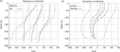
In this section, we investigate the model performance in reproducing the observed tidal and lower frequency velocity fluctuations at the Strait of Gibraltar. Figure 3a shows vertical profiles of the along-strait velocity at the Strait of Gibraltar (mean and mean ±1 standard deviation) as calculated from the WOCE1 and GE observations. Figure 3b shows similar vertical profiles but based on model simulations with (STIW1) and without (SNTW1) tidal oscillations. Figure 3a reproduces the already shown (Candela, 2001; Harzallah, 2009) larger velocities in WOCE1 compared to GE. When tide is used as a forcing the model satisfactorily reproduces the mean value and the amplitude of the oscillations. The largest discrepancies are found in the deepest layers. This is attributed in part to the model's coarse resolution that does not permit to reproduce detailed features of the very complex Strait topography. When tide is not used as forcing the simulated oscillations are much weaker and the baroclinic component of the flow dominates. One notices that the mean flow changes sign at smaller depths in the model (~100 m) compared to observations (~120–130 m) which again reflects a shallower strait bottom in the model compared to the actual one. Also one notices that the mean vertical profile presents a more pronounced shear in the simulation without tide than in the one with tide. This suggests that in the present simulations tidal oscillations reduce the baroclinic exchange. This fact will be discussed in detail in the following sections.

Fig. 3 Profiles of flow velocity at the Strait of Gibraltar (locations are shown in Fig. 2) with plus and minus one standard deviation. a) dashed–dotted lines: based on the WOCE1 measurements; continuous lines: based on the GE measurements. b) dashed–dotted lines: based on the simulation STIW1; dashed lines: based on the simulation SNTW1.

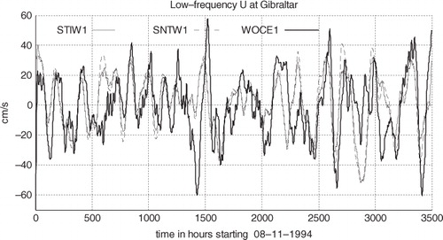
The simulated tide velocity at the Strait of Gibraltar (from STIW1 simulation) is compared to WOCE1 observations and to OTIS predictions. The comparison is shown as a scatter plot in Fig. 4. To retain only tidal oscillations, series are high-pass filtered (periods shorter than 42 hours are retained, cut-off frequency 4.1 10⁻⁵ rad s⁻¹). This frequency is found to be adequate for splitting the series into tidal and non-tidal components. A second order Butterworth filter (Butterworth, 1930) is used in the forward and backward directions successively to ensure a zero phase distortion. In this paper the Butterworth filter and the same cut-off frequency will be used in all filtering operations. The resemblance between the simulated tide and tide from WOCE1 is high with almost no lag and only a small reduction of the amplitude. Tide oscillations from OTIS show slightly weaker amplitude and present a phase shift. Hence it is concluded that the simulated tidal oscillations satisfactorily reproduce the observed ones at least compared to WOCE1 data. The lower frequency variability of the flow through Gibraltar is also compared to observations. The low-pass filtered series of the vertically averaged velocity at the Strait of Gibraltar are shown in Fig. 5. The figure compares the simulated velocity with and without tide forcing and the velocity based on WOCE1 data. The two simulated series are very close. Small differences can however be seen and could result as residuals of the filtering of the large tide oscillations. The resemblance between the simulated and observed velocities is high; most of the observed sub-inertial variability is reproduced by the model.

Fig. 4 Scatter plot of the high-pass filtered velocity at the Strait of Gibraltar (locations are shown in Fig. 2). Circles represent simulated velocities versus predicted ones using OTIS. Dots represent simulated velocities versus velocities based on the first WOCE sub period measurements. The simulation is STIW1 and the period considered is November 8, 1994 at 17:00 to April 3, 1995 at 08:00.

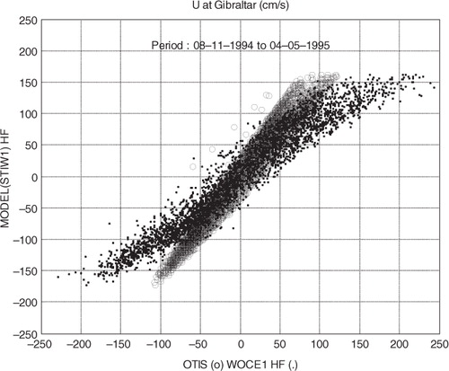
Fig. 5 Time series of the low-pass filtered velocity at the Strait of Gibraltar (locations are shown in Fig. 2). Continuous thick line: WOCE1 data first observing period. Continuous thin line: model simulation using tide as forcing at the Atlantic side (STIW1). Dashed thin line: model simulation without using tide as forcing (SNTW1). The period considered is November 8, 1994 at 17:00 to April 3, 1995 at 08:00.

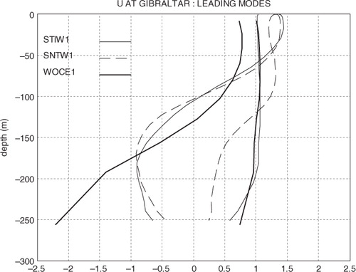
The two leading modes of variability of along-strait velocity at the Strait of Gibraltar are derived from the data sets and model outputs. The approach is similar to that in Harzallah (2009). Firstly, the barotropic mode is calculated and then removed from the series. In a second step, a baroclinic mode is derived with zero vertical average. The vertical profiles of modes 1 and 2 are shown in Fig. 6 from the two simulations with and without tide, STIW1 and SNTW1 and from WOCE1 data. The barotropic component (mode 1) is very similar in WOCE1 and STIW1. SNTW1 shows larger values in the upper layers and weaker values in the lower layer. On the other hand the baroclinic component is similar in the two simulations but, as mentioned, the reversal of the flow is shallower than in WOCE1. Modes 1 and 2 shown in Fig. 6 are similar to EOF modes obtained by Candela et al. (1989) and Vargas et al. (2006). As previously mentioned, largest discrepancy are found in the deep layers.

Fig. 6 Vertical profiles of the two derived modes of velocity at the Strait of Gibraltar (locations are shown in Fig. 2). Thick-continuous line: based on WOCE1 sub period measurements. Thin-continuous line: based on the simulation STIW1; thin-dashed line: based on the simulation SNTW1. The period is November 8, 1994 at 17:00 to April 3, 1995 at 08:00. Vertical profiles are standardised (rms=1).

The corresponding time series are shown in Fig. 7. At low frequency, the first mode series (Fig. 7a and c, white lines) are similar to the vertically averaged velocities shown in Fig. 5. For the second mode, STIW1 (Fig. 7b) and WOCE1 (Fig. 7d) show close variability; the time average in STIW1 is however slightly lower than in WOCE1. As mentioned before, this is in part attributed to differences in the Strait geometry. The second mode from SNTW1 is also shown in Fig. 7b. One notices that it follows the upper limit of the hourly fluctuations of STIW1. This indicates that the no-tide situation in the model corresponds to the maximum shear state and that at each tide oscillation the shear is lowered. In addition, the shear lowering is strongest during spring tides (e.g. abscissa around 2000) and weakest during neap tides (e.g. abscissa around 1800). As mentioned above, the lowering of the shear during spring tides and its increase during neap tides was shown by Candela et al. (1989), Vargas et al. (2006) and Harzallah (2009).

Fig. 7 Time series of velocity at the Strait of Gibraltar. a) hourly (black line) and low-pass filtered (white line) first-mode time series from STIW1. b) hourly (black line) and low-pass filtered (white line) second-mode time series from STIW1. The low-pass filtered second-mode from SNTW1 is also shown as thick black line. c) hourly (black line) and low-pass filtered (white line) first-mode time series from WOCE1. d) hourly (black line) and low-pass filtered (white line) second-mode time series from WOCE1. The period considered is November 8, 1994 at 17:00 to April 3, 1995 at 08:00.

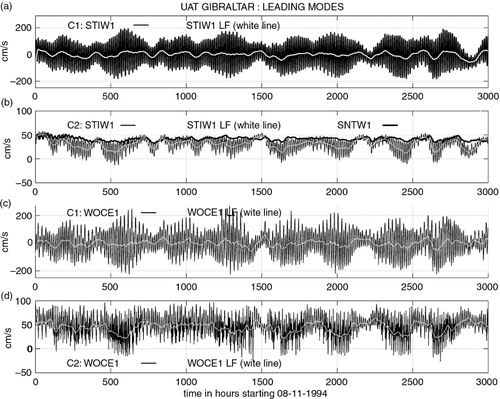
One also notices that the shear decreases in both STIW1 and SNTW1 when low frequency variability induced by the atmospheric forcing (atmospheric pressure) corresponds to an outflow state and increases when it corresponds to an inflow state. This behaviour is also observed in WOCE1. It is then deduced that the shear is the weakest during the simultaneous occurrence of spring tides and mean water outflow (e.g. abscissa around 2650) and the strongest during the simultaneous occurrence of neap tides and mean water inflow (e.g. abscissa around 1500). This result agrees with Vargas et al. (2006) who showed that the quasi-static transport in the upper layer is reduced and even reverses during spring tides and when the mean barotropic flow is towards the Atlantic. This also agrees with Tsimplis and Bryden (2000) who showed that at spring tides the interface is shallow and the outflow is maximal and at neap tides the interface is deep and the inflow is maximal.

The close relationship between the simulated time series and the observed ones shows that the model used is able to reproduce major features of the flow through the Strait of Gibraltar including the shear variability.

4. Tide and subinertial phases

In this section, we investigate the tide cycle at the Strait of Gibraltar in order to examine the time evolution relationship between the barotropic and baroclinic components of the flow and their interaction with low-frequency flow variability. The relationship with the density at the Strait of Gibraltar is also investigated. When possible, simulated cycles are compared to observed ones. Results from high-frequency filtered series and low-frequency filtered series are successively investigated. When performing correlations, the entire period hourly series are used (see Table 1). Furthermore, different relationships are investigated using lagged correlations. Positive (negative) lag for the correlation between the series C1 and C2, labelled C1C2, corresponds to C2 lagging C1 (C2 leading C1). C1 and C2 are modes one and two of velocity at the Strait and r refers to average density at the Strait. In a comparison (not shown) between the model and the observed densities at the Strait, the subinertial and tide fluctuations are found satisfactory resembling. The largest discrepancy is found for tidal amplitudes, being smaller in the simulation; phases are however well reproduced.

4.1. High-pass correlations

The observed and simulated velocity and density series are high-pass filtered. Lagged correlations are then calculated with lags ranging from −7 to +7 hours. The high-pass lagged correlations are shown in Fig. 8. The observed correlations between the first mode of velocity and the average density at the Strait, C1r, based on the GE data (Fig. 8a) show that the density is almost in opposite phase with the barotropic flow. The correlations reach very high values (~− 0.92) with 1-hour lag. Hence, the average density reaches its lowest value just after the flow is maxima towards the Mediterranean and highest values just after the flow is maxima towards the Atlantic. As already shown, this reflects vertical movements of the interface at the Strait of Gibraltar (Bryden et al., 1994).

Fig. 8 Lagged correlations between selected observed and simulated series high-pass filtered to focus on the tidal oscillations at the M2 time scale. The abscissa are leading and lagging hours. a) based on observations using WOCE1 and GE data; b) based on the simulation STIGE; c) based on the tide-alone simulation STAW1. Negative abscissa corresponds to the case that the second variable leads the first variable, and the opposite is for positive abscissa. Legends indicate each pair of time series involved in the calculation. C1 and C2 refer to the first and second modes of velocity at the Strait and r to the mean density at the Strait.

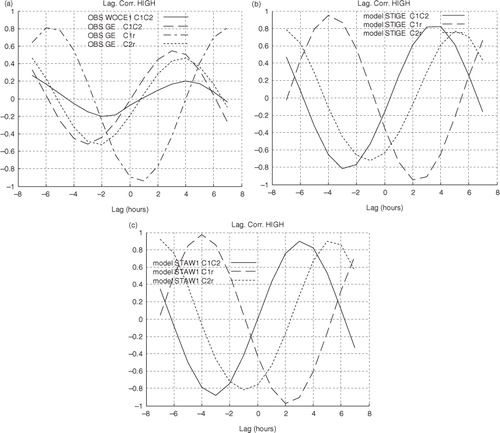
Figure 8a also shows relatively moderate correlations C1C2 (maximum ~+0.55) for the GE period. C2 lags C1 by approximately 3 hours (C1 and C2 are in quadrature phase). WOCE1 data show similar results but with much lower correlations (~+0.2 at a lag of 4 hours). C1 and C2 phase lags are such that flooding of the Mediterranean Sea is concomitant with maximum velocity shear and vice versa. This agrees with the description of tide structure at Camarinall Sill (e.g. Vargas et al., 2006). The correlations C2r resemble C1C2 with a 1-hour lag. The maximum correlation is −0.52 for r leading C2 by 2 hours.

Figure 8b shows lagged correlations from the model (GE period). Model results resemble observations but correlations are somewhat higher. The average density reaches minimum (C1r correlation of −0.92) at 2 hours lag. As for observations, C1C2 correlations are in quadrature phase but correlations are again high, higher than 0.8. Also as for observations, C2r correlations resemble those of C1C2 correlations but with a lag of 2 hours. Both observations and simulations show that density decrease, −r, lags barotropic inflow, C1, by 1–2 hours followed by shear increase, C2, also 1–2 hours later. The reverse sequence holds for the outflow. This sequence is clearly suggested in Fig. 8c where lagged correlations from the simulation with tide forcing alone are considered. The shear is enhanced during the flooding of the Mediterranean and reduced during the ebb. The above comparison shows that the main behaviour of the barotropic and baroclinic components of the flow at the Strait related to the tide forcing is well reproduced by the model.

4.2. Low-pass correlations

We now investigate the low-pass filtered lagged correlations. Figure 9a shows the lagged correlations based on the WOCE1 and GE observations. The time scale of correlations is around 4–6 d. This closely corresponds to the subinertial scale of the flow at Gibraltar (Candela et al., 1989). C1C2 correlations are relatively high for WOCE1 (+0.6) but weak for GE (+0.18). The reason for such a weak value is not obvious. On the other hand C1r correlations for GE are high (−0.88). One notices the almost no lag in C1C2 and -C1r (only 1 hour).

Fig. 9 Same as Fig. 8 but for selected observed and simulated series low-pass filtered to focus on the subinertial variability. a) based on observations using WOCE1 and GE data; b) based on the simulation STIGE; c) based on the simulation without tide SNTW1; d) based on the simulation where only tide is considered as a forcing STAW1. In d) the absolute value AC1 of the first mode C1 is used for correlations.

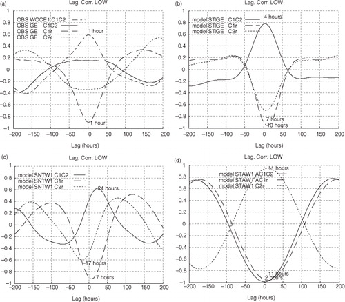
Figure 9b shows the lagged correlations based on the model simulation for the GE period. The correlations based on the simulation for the WOCE1 period are nearly the same and hence are not shown. C1C2 correlations have a maximum around 0.8 (4 hours lags). C1r correlations have a maximum of −0.96 (10 hours lag). Overall, the correlations based on the model are close to those based on observations. In addition both model and observations show very weak lags between correlation amplitudes. The lagged correlations based on the simulation without tide (SNTW1) are plotted in Fig. 9c. They show a sequence of occurrence of modes that recalls those shown by the high-pass filtered series (C1, then –r, then C2) but with larger lags. Indeed C2 lags C1 by 24 hours (maximum of 0.62), −r lags C1 by 7 hours (minimum of −0.9) and C2 lags −r by 17 hours (minimum of −0.6). This suggests that the subinertial fluctuations lead to similar behaviour at the Strait as that induced by the tidal oscillations but at a large time-scale. Differences between the correlations shown in Fig. 9b and c should result from tide oscillations effects on the longer time scales. The results suggest that at low frequencies, the tide effect is to reduce the time lag between the flow through Gibraltar and the shear.

To separate the effect of tide we plotted in Fig. 9d the correlations based on the simulation where only tide is considered (STAW1). As the low-pass part of C1 from this tide-alone simulation is weak (it represents tide residuals), the low-pass filtering is applied to the absolute value of C1, AC1. The time scale of correlations shown in Fig. 9d is around 12 d, which indicates that they are related to the fortnightly modulation of tide. AC1C2 and AC1r correlations are negative and high (close to −1); C2r correlations are positive and also high. All lags are rather small (2 hours for AC1C2 and 11 hours for AC1r and C2r). The high C2r correlations confirm that tide is responsible of the concomitant low-frequency oscillations of density and velocity shear.

The simulations performed with and without tide, together with the high-pass and low-pass correlations constitute powerful tools to investigate the interaction between tide and the subinertial variability at the Strait. It is shown that water flow generated by the low frequency atmospheric forcing or by high frequency tide oscillations both induce variations of density and of velocity shear. The water inflow leads to density reduction and velocity shear increase; the outflow leads to the reverse situation. Time intervals separating the flow, the density and the shear are 7 and 17 hours for the subinertial variability and 1 to 2 hours for tidal fluctuations. The interaction between tidal oscillations and the subinertial variability is strong; its effect is to reduce time lags so that the flow, the density and the shear variations appear almost concomitant.

5. Mass exchange

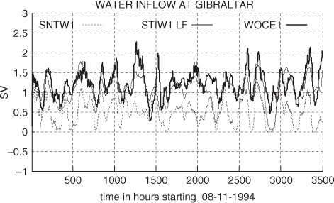
Time series of water exchanged at the Strait low-pass filtered is shown in Fig. 10. For this figure, the part corresponding to an input into (output from) the Mediterranean is calculated by setting to zero any negative (positive) velocity at the strait. One notes that this definition based on velocity shear differs from that usually used for Atlantic and Mediterranean water types. For example Sannino et al. (2004) derived a salinity distribution (based on a fortnightly average period) at the Strait that instantaneously defines the interface depth. The present definition takes into account the amount of water exchanged independently of its origin (Atlantic or Mediterranean). It is used here mainly for inflow (and outflow) comparison purposes based on simulations and observations. Figure 10 shows that when tide is considered, the simulated inflow series approaches the WOCE1 one. Although there is no appreciable change of the amplitude of fluctuations around mean values, tide does not induce a simple shift of the low-frequency transports but also interact with them. The correlation coefficient with the WOCE1 inflow increases from 0.45 to 0.62. The low-frequency fluctuations of the inflow and the outflow are more realistically simulated when tide is considered.

Fig. 10 Water fluxes into the Mediterranean basin through the Strait of Gibraltar. The simulated fluxes with tide STIW1 (continuous line) and without SNTW1 (dotted line) are shown. The water flux into the Mediterranean basin from WOCE1 is shown by a thick line. When calculating the fluxes into the Mediterranean basin, negative velocities are set to zero.

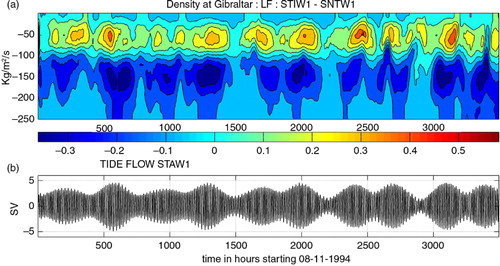
The effect of tide on the density at the Strait of Gibraltar is investigated by calculating the density difference between the simulations with tide (STIW1) and without tide (SNTW1). The density difference, plotted in Fig. 11a corresponds to an increase in the upper layers and a decrease in the lower layers. These changes are permanent features in time, but are more intense during spring tides (see Fig. 11b for time reference). The interface vertical movements explain such a density behaviour. In addition, the reduced Atlantic inflow in the upper layers and outflow in the lower layers (as result of the shear decrease during spring tides, Fig. 7) and the enhanced mixing of Atlantic and Mediterranean waters may also contribute to it.

Fig. 11 a) low-pass filtered difference of density (kgm^-3) at the Strait of Gibraltar between simulations STIW1 and SNTW1. The figure is shown as a time-depth Hovmöller diagram. b) for time reference, tide flow is shown as the mean water transport from the simulation where only tide is considered as forcing (STAW1, in Sv).

The barotropic and baroclinic components of the mass flux obtained using the velocity reconstructed from modes 1 and 2 and low-pass filtered are shown in Fig. 12a and b. These fluxes are based on the tide-alone simulation, STAW1. The vertical profile for a neap tide state (time number 2919) is subtracted to obtain deviations relative to an almost no tide state. This date is chosen as the corresponding tide amplitude is the weakest simulated. For time reference the volume flux from the tide-alone simulation is shown in Fig. 12c. Tidal oscillations induce a mass flux to the Mediterranean with largest values during the spring tide phase. This mass flux is nearly the same over the entire water column. The baroclinic mode shows weakening of the mass exchange both in the upper and lower layers with largest values during spring tides. As mentioned earlier, the opposite direction changes of modes 1 and 2 were found in Harzallah (2009) based on the WOCE1 and GE data; they were explained by a dynamical equilibrium between the two. It should be noted that some monthly variability is simulated in the two modes. Such variability was previously shown in Vargas et al. (2006).

Fig. 12 a) mass flux through the Strait of Gibraltar (in kg m⁻² s⁻¹) reconstructed using the first mode of velocity low-pass filtered based on the simulation with tide alone (STAW1). The vertical profile for a neap tide state (the vertical profile at time number 2919) is subtracted to obtain deviations relative to an almost no tide state (the neap tide state). b) as a) but for the second mode. c) for time reference, the tide flow is shown as the mean water transport from the simulation where only tide is considered as forcing (STAW1). d) Difference of mass flux reconstructed with mode 1 of velocity between the tidal (STIW1) and no tidal (SNTW1) simulations, low-pass filtered (in kg m⁻² s⁻¹). e) as d) but for mode 2. f) for time reference, the subinertial flow induced by external forcing (first velocity mode from SNTW1, in cm/s).

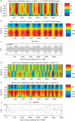
The above mass fluxes are derived for tide oscillations alone. To investigate the interactions between tide and the subinertial variability, the mass fluxes reconstructed based on the two leading modes from the STIW1 and SNTW1 simulations are calculated and low-pass filtered. Their differences are plotted in Fig. 12d and e. For time reference the simulated velocity series induced by external forcing (first velocity mode from SNTW1) are shown in Fig. 12e. For the baroclinic component, Fig. 12e reproduces the mass flux exchange reduction during spring tides by tidal oscillations as shown in Fig. 12b but altered by the lower frequency oscillations. The alteration is such that the mass fluxes in both directions are reduced by tidal oscillations when the flow induced by external forcing is towards the Atlantic and increased when it is towards the Mediterranean but the increase is weak and limited in time. Again, tide not only reduces the exchange through the strait with maximum reduction during the spring phase but also interacts with the lower-frequency mean flow further reducing the exchange when the flow is towards the Atlantic. The barotropic mode (Fig. 12d) shows a similar behaviour but with opposite sign and higher frequency fluctuations.

The mean values of the mass flux calculated for the simulations STAW1, SNTW1 and STIW1 and for the GE data show that the baroclinic component of the subinertial and tide oscillations (C2) both induce a net mass loss, but that induced by subinertial oscillations is larger (−0.34±0.11 and −0.41±0.08 kg m⁻² s⁻¹ for tide and subinertial oscillations, respectively). The superimposition of the two baroclinic oscillations induces even a lower net mass loss (−0.28±0.14 kg m⁻² s⁻¹) close to the net mass loss from GE observations (−0.26±0.14 kg m⁻² s⁻¹). Hence, the barotropic tidal oscillations damp the baroclinic mass loss. It is to mention that it was not possible to provide an accurate estimate of the mean mass flux for C1 due to large fluctuating series.

6. Impacts on the thermohaline circulation

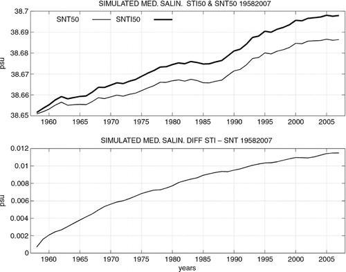
In this section we investigate the impact of tidal oscillations on the thermohaline circulation in the Mediterranean Sea. As presented above two parallel simulations are conducted with (STI50) and without (SNT50) tide. The simulations have duration of 50 yr, from 1958 to 2007. The Mediterranean Sea potential temperature series (water volume average) from these two simulations are shown in Fig. 13 together with their differences. The two temperature series start from the same state but temperatures are lowered when tide is included. The difference between series corresponds to a rather regular decrease although the variation rate seems lower at the end of the simulations. The difference reaches nearly −0.08°C after 50 yr. Similarly, the simulated salinity series are shown in Fig. 14. Tide increases the Mediterranean water salinity. The difference between series increases but slowly tends to a limit value. At the end of the simulations the increase is around +0.012 psu.

Fig. 13 Upper panel: Potential temperature averaged over the entire Mediterranean volume from the 50-yr simulations. Thick curve: tide is used as forcing; thin curve: without tide. Lower panel: their difference.

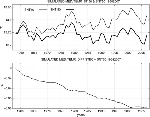
Fig. 14 Same as in Fig. 13 but for the average salinity.

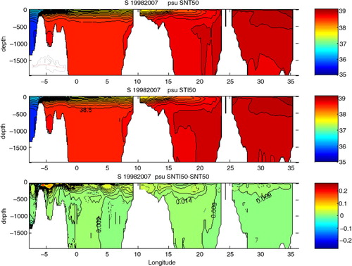
The temperature and salinity from the two simulations (average over the last 10 yr; 1998–2007) and their differences are shown in Figs. 15 and 16, respectively, as vertical sections extending between the western and the eastern sides of the Mediterranean. The temperature decrease by tidal oscillations reaches almost the entire Mediterranean with the largest values in the intermediate layers. Cooler waters enter the Mediterranean Sea in the upper layers of the Strait of Gibraltar and then move eastward and fill the Mediterranean basin, especially the upper 250 m in the western part of the western basin and deeper layers further east. Figure 16 shows that higher salinity waters enter the Mediterranean Sea when tide is considered. These waters are found at shallow depths even in the eastern basin. At the Strait of Gibraltar Figs. 15 and 16 clearly show that upper layer waters are cooled and saltened whereas deeper layer waters are warmed and freshened which reflects an increased mixing in the Strait.

Fig. 15 Average potential temperature over the 10-yr period 1998–2007 from simulations STI50 (upper panel) and SNT50 (middle panel) and their differences (lower panel). Panels are shown along east–west vertical sections. The horizontal location of the section is presented on the lower left corner of the upper panel.

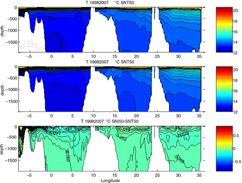
Fig. 16 As Fig. 15 but for salinity.

The mean net water flux entering the Mediterranean from the Atlantic equals the mean net water loss at the surface and is therefore unchanged when the tide is considered. On the other hand the mean net heating of the Mediterranean at the Strait is lowered from 4.0 Wm⁻² without tide to 3.3 Wm⁻² with tide (mean values over the 50-yr period). This reflects the cooling of the Mediterranean basin shown above. The mean heat loss at the sea surface, which equals −4.1 Wm⁻² without tide, is reduced to −3.3 Wm⁻² with tide. This reduction occurs through the relaxation fluxes at the surface. The model is therefore able to adjust the surface fluxes to fluxes at the Strait of Gibraltar through adjustment to changes of the surface temperatures. The mean net salt flux at the Strait of Gibraltar increases from 0.53 to 0.59 psu.ms⁻¹, which reflects the saltening of the Mediterranean basin.

At the Strait, the increased salinity waters located over the decreased salinity ones agree with the model results shown by Sannino et al., 2004. The authors examined the salinity change east of the Camarinal sill when a tide is added (M2 and S2 components). They attributed the increased salinity to an increased entrainment of Mediterranean waters in the upper layer and the lowered salinity to an increased entrainment of the Atlantic waters in the denser layer. The changes also agree with García Lafuente et al. (2013) who showed thicker interface and hence water mixing layers extending from nearly 300 m depth west of the sill to nearly 150 m depth east of the sill. A thicker interface corresponds to increased salinity of the inflowing waters above the lowered salinity of the outflowing waters.

An additional simulation (20 d, SNTS20) was performed where the temperature and salinity at the Strait between 5.5 and 6.2°W are slightly smoothed (with a relaxation toward the east–west segment average at each time step at a rate of 0.016% s⁻¹). In this simulation tide is not used as forcing. The velocity shear is compared to the simulation with no smoothing and without tide (20 d, SNT20) and to the simulation with no smoothing but with tide (20 d, STI20). Results (not shown) reveal that the velocity magnitude in SNTS20 decreases in the upper and lower layers similar to the decrease due to tide (STI20). Compared to the no tide case (SNT20), the shear is lowered by around 28% in STI20 and 31% in SNTS20 but this ratio is dependent on the smoothing magnitude. Hence in the model, a simple mixing of waters at the strait damps the thermohaline exchange.

The decrease of temperatures and increase of salinity shown above is explained by the mixing at the Strait which leads to a recirculation of waters crossing the Strait and hence acts as an inhibiting mechanism of the renewal of Mediterranean waters. If one hypothetically considers larger tide fluctuations at the strait, the mixing will be enhanced and the exchange reduced. A hypothetical limit may be reached with complete mixing and recirculation of the water crossing the strait; the exchange is inhibited and the Mediterranean Sea is disconnected from the Atlantic Ocean. With no heat and salt fluxes at the Strait, the Mediterranean Sea is homogenised vertically with lower temperatures and higher salinities, hence reducing or even stopping the heat loss at the sea surface. The Mediterranean progressively tends to an isolated homogenous body of water. This limit may recall the ‘overmixed’ limit where density difference is reduced by water recirculation inside the sea (Bryden and Stommel, 1984, Garrett et al., 1990). This hypothetical limit is based on the INSTMED06 model results; the actual Mediterranean behaviour may be different and further modelling tests with longer periods are needed. On the other side, not including tides in numerical models, which is the case of most present-day Mediterranean Sea models, leads to water exchange free from any tide mixing which corresponds to an exaggerated heat and salt exchange both at the Strait and at the Sea surface and to an increased Mediterranean thermohaline circulation. Model tuning (e.g. Sannino et al., 2009) or adding dissipation (Hibiya and Leblond, 1993; Hibiya et al., 1998) generally permits to numerically overcome this effect.

7. Conclusion

The Strait of Gibraltar is a region that connects the Mediterranean Sea to the Atlantic Ocean through highly complex dynamical processes. The numerical simulation of the exchange at the Strait constitutes a challenge; both barotropic and baroclinic flow components should be taken into account. The subinertial variability ranging from days to months is also of high importance. In addition tide induces intense water fluxes at short time scales of a few hours with strong interaction with the Strait bathymetry. A realistic representation of the bathymetry in numerical models is needed.

A numerical model of the Mediterranean Sea with resolution increased at the Strait of Gibraltar where the Strait width is represented by three grid points is shown to successfully reproduce the main features of the flow including those related to tide. Roles of the low frequency variability and of the higher frequency tidal oscillations can be clearly examined using the model with different forcing settings. Using tidal oscillations or the subinertial variability as separate forcing fields permit to isolate their roles whereas considering the difference between the simulation with both forcing and the simulation forced by the subinertial variability alone permits to examine dynamical interactions between the two forcing.

One of the major observed dynamical behaviours of the flow at the Strait of Gibraltar, the fortnightly modulation of the baroclinic component with shear decrease during spring tides and increase during neap tides, is reproduced by the model. In addition, the simulations showed that the shear oscillations related to tide represents a decrease from a maximum corresponding to the shear state without a tide forcing. Moreover, as for observations the model reproduces the shear decrease when the mean flow is towards the Atlantic.

The model also reproduces the previously shown opposite direction mass fluxes of the barotropic and baroclinic components. It is shown that tidal oscillations induce a mass flux to the Mediterranean almost over the entire water column with the largest values during the spring tide phase. At the opposite the baroclinic mode shows weakening of the mass exchange in both upper and lower layers with the largest values during spring tides. The simulations show that the baroclinic mass flux reduction by tidal oscillations during spring tides is altered by the lower frequency oscillations with further reduction when the flow induced by external forcing is towards the Atlantic.

The different phases of the simulated tidal flow at the Strait also show a resemblance with observations. At high frequency both observations and the simulations show that the density decrease lags barotropic inflow by 1–2 hours followed by a shear increase also 1–2 hours later, and the reverse situation for the outflow. The shear is enhanced during the flooding of the Mediterranean and reduced during the ebb. Similar to the shear reduction by tide fluctuations, the simulations show that water inflow generated by the low frequency atmospheric forcing induce a velocity shear increase preceded by a lowering of the density. The inverse situation holds for the outflow. The lag between the density and shear variations with respect to the subinertial variability is reduced by tide. Indeed, observations and the simulation with both forcing show a nearly concomitant behaviour of the barotropic and baroclinic components of the flow and of the density when tide is included.

Tidal oscillations advect water at almost all layers including that previously leaved the basin. The resulting enhanced mixing at the Strait of Gibraltar reduces the gradient between the Mediterranean basin and the Atlantic Ocean. The exchange alteration is increased during spring tides and reduced during neap tides. Hence the water entering the Mediterranean is cooler on average. In the same way the mixing at the strait induces more saline waters entering the basin and less saline waters leaving it. Multi-decadal simulations also show that the Mediterranean basin is cooled and saltened by the tide. Maximum changes in the Mediterranean Sea are shown to occur in the upper and intermediate layers leading to more homogenised waters.

The present study shows that tide may be an important factor of the forcing of the Mediterranean Sea basin. Any effect on the basin water characteristics including the surface ones may in turn act on the atmosphere above the Mediterranean Sea interface. One major concern when modelling the Mediterranean Sea is how the Atlantic Ocean is considered. For most present-day models a buffer zone with relaxation toward varying or climatic hydrographic characteristics is used. Close to the western side of the Strait the relaxation time scale determines how strong is the exchange and also defines the density gradient through the Strait. In general, the relaxation time scale is tuned so as the model water exchange approaches the admitted value. The effect of cooling and saltening of the Mediterranean Sea by tidal oscillations found here is probably sensitive to the relaxation time scale. Viscosity and diffusivity parameterisations in the Strait may also have an impact on the model results. It is important to test other horizontal advection schemes that are conservative and less diffusive as the Smolarkiewicz (1984) scheme, also used in Sannino et al. (2002, 2004). The dynamical boundary conditions in the Atlantic Ocean area also play an important role on the simulation of tide. It is important to compare the results obtained here using open lateral boundary conditions to those using volume-conservation models. The geographical extension of the Atlantic buffer zone may also play a role on the tide exchange. It is important that dynamical boundary conditions do not generate unrealistic structures in the buffer zone that may interact with the flow in the Strait. This is particularly important in view of the very energetic tidal dynamics. Concerning the tidal impact on the Mediterranean Sea thermohaline circulation, the results presented here should be regarded as preliminary ones as they are based on one single model with relatively low resolution. It is important to compare the present work results to results from other Mediterranean Sea models in particular eddy-resolving models with higher horizontal and vertical resolution (Stanev and Staneva, 2001). It is also important to test other atmospheric forcing approaches as the use of surface meteorological parameters or Mediterranean Sea models coupled to the atmosphere with complete sea–atmosphere feedbacks.

References

- Alioua M. , Harzallah A . Imbrication d'un modèle de circulation des eaux près des côtes tunisiennes dans un modèle de circulation de la mer Méditerranée [Nesting of a water circulation model along the Tunisia coasts in a Mediterranean Sea model]. Bull. Inst. Nat. Sci. Tech. Mer de Salammb. 2008; 35: 169–176.
- Arabelos D. N. , Asteriadis G. , Contadakis M. E. , Papazachariou D. , Spatalas S. D . Assessment of recent tidal models in the Mediterranean Sea. Dynamic Planet. Int. Assoc. Geodesy Sumposia. 2007; 130: 57–62.
- Arabelos D. N. , Papazachariou D. Z. , Contadakis M. E. , Spatalas S. D . A new assimilation tidal model for the Mediterranean Sea. Ocean Sci. Discuss. 2010; 7: 1703–1737.
- Armi L. , Farmer D. M . The flow of Atlantic water through the Strait of Gibraltar. Progr. Oceanogr. 1988; 21(1): 1–105.
- Astraldi M. , Boulopoulos S. , Candela J. , Gacic M. , Gasparini G. P. , co-authors . The role of straits and channels in understanding the characteristics of the Mediterranean circulation. Progr. Oceanogr. 1999; 44(1–3): 65–108.
- Brankart J.-M. , Pinardi N . Abrupt cooling of the Mediterranean Levantine Intermediate Water at the beginning of the 1980s: observational evidence and model simulation. J. Phys. Oceanogr. 2001; 31(8): 2307–2320.
- Brasseur P. , Beckers J.-M. , Brankart J.-M. , Schoenauen R . Seasonal temperature and salinity fields in the Mediterranean Sea: climatological analyses of an historical data set. Deep-Sea Res. 1996; 43(2): 159–192.
- Bryden H. L. , Candela J. , Kinder T. H . Exchange through the strait of Gibraltar. Progr. Oceanogr. 1994; 33(3): 201–248.
- Bryden H. L. , Stommel H. M . Limiting processes that determine basic features of the circulation in the Mediterranean Sea. Oceanol. Acta. 1984; 7: 289–296.
- Butterworth S . On the theory of filter amplifiers. Wireless Eng. 1930; 7: 536–541.
- Candela J . The Gibraltar strait and its role in the dynamics of the Mediterranean Sea. Dynamics of the Atmospheres and Oceans. 1991; 15(3–5): 12267–12299.
- Candela J . Siedler G. , Church J. , Gould J . Mediterranean water and global circulation. Ocean Circulation and Climate: Observing and Modelling the Global Ocean.
- Candela J. , Winant C. D. , Ruiz A . Tides in the strait of Gibraltar. J. Geophys. Res. 1990; 95(C5): 7313–7335.
- Chioua J. , Bruno M. , Vázquez A. , Reyes M. , Gomiz J. J. , co-authors . Internal waves in the Strait of Gibraltar and their role in the vertical mixing processes within the Bay of Algeciras. Estuar. Coast. Shelf Sci. 2013; 126: 70–86. DOI: http://dx.doi.org/10.1016/j.ecss.2013.04.010.
- Dee D. P. , Uppala S. M. , Simmons A. J. , Berrisford P. , Poli P. , co-authors . The ERA Interim reanalysis: configuration and performance of the data assimilation system. Q. J. Roy. Meteorol. Soc. 2011; 137: 553–597.
- Dressler R . Hydrodynamisch-numerische Untersuchungen der M2 Gezeit und einiger Tsunamis im eurpaishen Mittelmer [Numerical investigations of the hydrodynamic of the M2 tide and of some Tsunamis in the European Mediterranean Sea] .
- Egbert G. D. , Erofeeva S. Y . Efficient inverse modeling of barotropic ocean tides. J. Atmos. Oceanic Technol. 2002; 19(2): 183–204.
- Fenoglio-Marc L. , Mariotti A. , Sannino S. , Meyssignac B. , Carillo A. , co-authors . Decadal variability of net water flux at the Mediterranean Sea Gibraltar Strait. Glob. Planet. Change. 2013; 100: 1–10.
- García Lafuente J. , Bruque Pozas E. , Sánchez Garrido J. C , Sannino G. , Sammartino S . The interface mixing layer and the tidal dynamics at the eastern part of the Strait of Gibraltar. J. Mar. Syst. 2013; 117–118: 31–42.
- García Lafuente J. , Delgado J. , Criado F . Inflow interruption by meteorological forcing in the Strait of Gibraltar. Geophys. Res. Lett. 2002b; 29(19): 1914.
- García Lafuente J. , Vargas J. M. , Delgado J. , Criado F . Subinertial and seasonal variability in the Strait of Gibraltar from CANIGO observations. The 2nd meeting on the Physical Oceanography and Sea Straits. 2002a; Villefranche. 15–19. April 2002.
- Garrett C. J. , Bormans M. , Thompson K . Pratt K.J . Is the exchange through the Strait of Gibraltar maximal or submaximal?. 1990; Boston: Kluwer Academic Publishers. 271–294. In: The Physical oceanography of Sea Straits.
- Gualdi S. , Somot S. , Wilhelm May W. , Castellari S. , Déqué M. , co-authors . Navarra A. , Tubiana L . Future climate projections. Regional Assessment of Climate Change in the Mediterranean. 2013; Dordrecht, The Netherlands: Springer. 53–118.
- Haney R. L . On the pressure gradient force over steep topography in sigma coordinate ocean models. J. Phys. Oceanogr. 1991; 21: 610–619.
- Harzallah A . Flow variability in the Strait of Gibraltar: the Mediterranean adjustment to tidal forcing. Deep-Sea Res. I. 2009; 56(2009): 459–470.
- Herrmann M. , Somot S . Relevance of ERA40 dynamical downscaling for modeling deep convection in the Mediterranean Sea. Geophys. Res. Lett. 2008; 35: L04607.
- Herrmann M. , Somot S. , Sevault F. , Estournel C. , Déqué M . Modeling the deep convection in the northwestern Mediterranean Sea using an eddy-permitting and an eddy resolving model: case study of winter 1986–87. J. Geophys. Res. 2008; 113: C04011.
- Hibiya T. , Leblond P. H . The control of fjord circulation by fortnightly modulation and tidal mixing processes. J. Phys. Oceanogr. 1993; 23: 2042–2052.
- Hibiya T. , Ogasawara M. , Niwa Y . A numerical study of the fortnightly modulation of basin-ocean water exchange across a tidal mixing zone. J. Phys. Oceanogr. 1998; 28: 1224–1235.
- Hourdin F. , Musat I. , Bony S. , Braconnot P. , Codron F. , co-authors . The LMDZ4 general circulation model, climate performance and sensitivity to parametrized physics with emphasis on tropical convection. Clim. Dynam. 2006; 27: 787–813.
- Lacombe H. , Richez C . Hydrology and currents in the Strait of Gibraltar. Office of Naval Research. Sea Straits Rep. 1984; 51 figures, NORDA.
- L'Hévéder B. , Li L. , Sevault F. , Somot S . Interannual variability of deep convection in the Northwestern Mediterranean simulated with a coupled AORCM. Clim. Dynam. 2013; 41: 937–960.
- Li Z. X . Ensemble atmospheric GCM simulation of climate interannual variability from 1979 to 1994. J. Clim. 1999; 12: 986–1001.
- Macias D. , García C. M. , Echevarría Navas F. , Vázquez-López-Escobar A. , Bruno Mejías M . Tidal induced variability of mixing processes on Camarinal Sill (Strait of Gibraltar): a pulsating event. J. Mar. Syst. 2006; 60: 177–192.
- Mertens C. , Schott F . Interannual variability of deep-water formation in the northwestern Mediterranean. J. Phys. Oceanogr. 1998; 28: 1410–1424.
- Mellor G. L . A Three Dimensional Primitive Equation Numerical Ocean Model.
- Mellor G. L. , Ezer T. , Oey L.-Y . The pressure gradient conundrum of sigma coordinate ocean models. J. Atm. Ocean. Tech. 1994; 11: 1126–1134.
- Mellor G. L. , Yamada T . Development of turbulent closure model for geophysical fluid problems. Rev. Geophys. 1982; 20: 851–875.
- Morozov E. G. , Trulsen K. , Velarde M. G. , Vlasenko V. I . Internal tides in the strait of Gibraltar. J. Phys. Oceanogr. 2002; 32: 3193–3206.
- Pillsbury R. D. , Barstow D. , Bottero J. S. , Milleiro C. , Moore B. , co-authors . Gibraltar Experiment, current measurements in the Strait of Gibraltar, October 1985–October 1986. 1987; 284pp. Oregon State University Data Report 87–29, Ref. 139, College of Oceanography.
- Rojas M. , Li L. Z. , Kanakidou M. , Hatzianastassiou N. , Seze G. , co-authors . Winter weather regimes over the Mediterranean region: their role for the regional climate and projected changes in the 21st century. Clim. Dynam. 2013; 41: 551–571.
- Sanchez B. V. , Ray R. , Cartwright D. E . A Proudman-function expansion of the M2 tide in the Mediterranean Sea from satellite altimetry and coastal gauges. Oceanol. Acta. 1992; 15: 325–337.
- Sánchez-Garrido J. C. , Sannino G. , Liberti G. , García Lafuente J. , Pratt L . Numerical modeling of three-dimensional stratified tidal flow over Camarinal Sill, Strait of Gibraltar. J. Geophys. Res. 2011; 116: 12026.
- Sanchez-Gomez E. , Somot S. , Josey S. A. , Dubois C. , Elguindi N. , co-authors . Evaluation of Mediterranean Sea water and heat budgets simulated by an ensemble of high resolution regional climate models. Clim. Dynam. 2011; 37: 2067–2086.
- Sánchez-Román A. , Criado-Aldeanueva F. , GarcIá-Lafuente J. , Garrido J. S . Vertical structure of tidal currents over Espartel and Camarinal sills, Strait of Gibraltar. J. Mar. Syst. 2008; 74: 120–133.
- Sánchez-Román A. , García-Lafuente J. , Delgado J. , Sánchez-Garrido J. C. , Naranjo C . Spatial and temporal variability of tidal flow in the Strait of Gibraltar. J. Mar. Syst. 2012; 98–99: 9–17.
- Sánchez-Román A. , Sannino G. , GarcIá-Lafuente J. , Carillo A. , Criado-Aldeanueva F . Transport estimates at the western section of the Strait of Gibraltar: a combined experimental and numerical modelling study. J. Geophys. Res. 2009; 114: C06002.
- Sannino G. , Bargagli A. , Artale V . Numerical modeling of the mean exchange through the Strait of Gibraltar. J. Geophy. Res. 2002; 107(C8): 3094.
- Sannino G. , Bargagli A. , Artale V . Numerical modeling of the semidiurnal tidal exchange through the Strait of Gibraltar. J. Geophys. Res. 2004; 109: 05011.
- Sannino G. , Herrmann M. , Carillo A. , Rupolp V. , Ruggiero V. , co-authors . An eddy-permitting model of the Mediterranean Sea with a two-way grid refinement at the Strait of Gibraltar. Ocean Model. 2009; 30: 56–72.
- Smith W. H. F. , Sandwell D. T . Global seafloor topography from satellite altimetry and ship depth soundings. Science. 1997; 277: 1957–1962.
- Smolarkiewicz P. K . A fully multidimensional positive definite advection transport algorithm with small implicit diffusion. J. Comput. Phys. 1984; 54: 325–362.
- Stanev E. V. , Staneva J. V . The sensitivity of the heat exchange at sea surface to meso and sub-basin scale eddies. Model study for the Black Sea. Dynam. Atmos. Oceans. 2001; 33: 163–189.
- Tsimplis M. N. , Bryden H. L . Estimation of the transports through the Strait of Gibralta. Deep-Sea Res. I. 2000; 47: 2219–2242.
- Tsimplis M. N. , Proctor R. A. , Flather A . A two-dimensional tidal model for the Mediterranean Sea. J. Geophys. Res. 1995; 100(C8): 16223–16239.
- Vargas J. M. , García-Lafuente J. , Candela J. , Sánchez A . Fortnightly and monthly variability of the exchange through the Strait of Gibraltar. Progr. Oceanogr. 2006; 70: 466–485.
- Vázquez A. , Miguel M. , Izquierdo A. , MacIás D. , Ruiz-Cañavate A . Meteorologically forced subinertial flows and internal wave generation at the main sill of the Strait of Gibraltar. Deep-Sea Res. I. 2008; 55(2008): 1277–1283.
- Vincent P. , Canceill P . Oceanic tides in the Mediterranean Sea. Int. Geoid Serv. Bull. 1993. 2, 84–90, D.I.I.A.R., Politecnico di Milano, Italy.
- Vorosmarty C. J. , Fekete B. M. , Tucker B. A . Global River Discharge, 1807–1991, Version. 1.1 (RivDIS). 1998. Data set. Available on-line [http://www.daac.ornl.gov] from Oak Ridge National Laboratory Distributed Active Archive Center, Oak Ridge, Tennessee, U.S.A.
- Wang D.-P . Model of mean and tidal flows in the Strait of Gibraltar. Deep-Sea Res. 1989; 36: 1535–1548.
- Wesson J. C. , Gregg C . Mixing at the Camarinal sill in the Strait of Gibraltar. J. Geophys. Res. 1994; 99(C5): 9847–9878.