Assessment of a zoomed global model for the North Sea by comparison with a conventional nested regional model

Abstract

Assessment of marine downscaling of global model simulations to the regional scale is a prerequisite for understanding ocean feedback to the atmosphere in regional climate downscaling. Major difficulties arise from the coarse grid resolution of global models, which cannot provide sufficiently accurate boundary values for the regional model. In this study, we first setup a stretched global model (MPIOM) to focus on the North Sea by shifting poles. Second, a regional model (HAMSOM) was performed with higher resolution, while the open boundary values were provided by the stretched global model. In general, the sea surface temperatures (SSTs) in the two experiments are similar. Major SST differences are found in coastal regions (root mean square difference of SST is reaching up to 2°C). The higher sea surface salinity in coastal regions in the global model indicates the general limitation of this global model and its configuration (surface layer thickness is 16 m). By comparison, the advantage of the absence of open lateral boundaries in the global model can be demonstrated, in particular for the transition region between the North Sea and Baltic Sea. On long timescales, the North Atlantic Current (NAC) inflow through the northern boundary correlates well between both model simulations (R~0.9). After downscaling with HAMSOM, the NAC inflow through the northern boundary decreases by ~10%, but the circulation in the Skagerrak is stronger in HAMSOM. The circulation patterns of both models are similar in the northern North Sea. The comparison suggests that the stretched global model system is a suitable tool for long-term free climate model simulations, and the only limitations occur in coastal regions. Regarding the regional studies focusing on the coastal zone, nested regional model can be a helpful alternative.

• regional ocean model
• global ocean model
• North Sea
• HAMSOM
• MPIOM
• marine downscaling

1. Introduction

Downscaling of global climate model estimates to the North Sea is undergoing a rapid development in this century (Janssen et al., 2001; Schrum, 2001; Schrum et al., 2003; Weisse et al., 2009; Holt et al., 2010). The evaluation of a complex climate model should be initially carried out at the module level, that is, by isolating particular components (e.g. atmosphere, ocean and ice modules) and testing them independently by the fully coupled model (IPCC, 2007). Hence, the quality of the model components should be validated on a decadal time scale before performing the regional climate downscaling (Griffies et al., 2000). The conventional way to perform the marine downscaling is by interpolating the coarse grid global model information to the open boundaries of the regional high-resolution model. This method leads to discussion about the choice of open boundary conditions (Palma and Matano, 1998; Marchesiello et al., 2001; Chen et al., 2013). Ådlandsvik and Bentsen (2007) performed the marine downscaling of global simulations to the North Sea from a coupled climate model (20C3M experiment). They reported that the added value of downscaling is to provide the regional details, doubling the Atlantic inflow to the North Sea, and improving the mean winter temperature. Regional ocean climate simulations were also evaluated for the Baltic Sea (Meier, 2002; Meier and Kauker, 2003). Their model system was shown to remain stable over decades without bias correction and realistically simulated the time evolution of the halocline over a long period. The coarse resolution of global models often entails unreasonable boundary values, compelling the application of a bias correction (Mathis et al., 2013). Compared to conventional one-way nested models, variable-resolution GCMs gain more attention recently (see McGregor, 2013, and references therein). A major model intercomparison project, the Stretched Grid Model Intercomparison Project (SGMIP, Fox-Rabinovitz et al., 2006, 2008), demonstrated that benefits of the variable-resolution global approach include the absence of any lateral boundaries and the related problems with spurious reflections.

In recent studies, the Max Planck Institute Ocean Model (MPIOM) has been successfully applied for the regional climate studies by using an orthogonal curvilinear C-grid with shifted poles (Marsland et al., 2003). The poles are chosen to yield a high horizontal resolution in the region of interest, while maintaining a global model domain devoid of open boundary problems experienced in regional models, for example, the study in the East Antarctica (Marsland et al., 2004), the Arctic (Mikolajewicz et al., 2005) and the Indonesian Seas (Aldrian et al., 2005). However, the minimum thickness of the first layer in a tidal resolving global model has to be of the order of 15 m. Due to this limitation, it is not possible to adequately resolve coastal dynamical processes. Moreover, a higher resolution to resolve dynamics in coastal regions and estuaries with a global model is too expensive. Therefore, we also applied the conventional nested regional model as a reference model in this study. By comparing with this well-validated regional model, we can answer questions concerning the accuracy of global models for different properties on the decadal scale.

The circulation at the northern entrance of the North Sea, where the main exchange between the North Sea and North Atlantic occurs, has been studied for a long time (Dooley, 1974; Svendsen et al., 1991; Turrell et al., 1992; Winther and Johannessen, 2006). In this region, the coarse resolution global model cannot resolve well, thus it leads to poor regional model results in the northern North Sea. The general circulation pattern in the North Sea is cyclonic. The inflow of Atlantic water has several branches and follows different pathways. The inflow between the Orkney and Shetland Islands continues southward and mixes with fresh waters from the British east coast. The eastern inflow follows the western slope of the Norwegian Trench (East Shetland current, ESC) and meets brackish water in the inner Skagerrak, where it returns northwards. The northward current, enhanced by freshwater introduced along the Norwegian coast, is defined as the Norwegian coastal current (NCC, Rodhe, 1996; Winther and Johannessen, 2006). The dominant decadal variation over the North Atlantic can be related to the North Atlantic Oscillation (NAO) (Hurrell, 1995). Nevertheless, Meyer et al. (2011) confirmed in their study that local air-sea interactions are the main drivers of the decadal heat content variability in the North Sea. However, a detailed study concerning conditions under which the decadal signal can be transported from global models into the North Sea is still lacking in the literature (Albretsen and Røed, 2010).

In this work, we compare two different marine downscaling experiments for the North Sea. First, we use a stretched global model MPIOM, and secondly the nested regional model HAMSOM as a reference. Both models have been well validated and used in different regions of the world for a variety of applications. For the first set of experiments, the MPIOM model was setup with a focus on the North Sea (zooming). For the second set of experiments, the HAMSOM model was adapted with higher resolution in the North Sea, using open boundary values interpolated from the MPIOM results (nesting). By evaluating hindcast experiments using these two model settings, we aim to obtain insight into the specific characteristics of both systems and whether they could be used in a free climate model simulation for regional focus.

2. Methods

2.1. The MPIOM global model

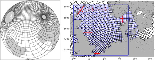
MPIOM is the ocean component of the Max-Planck-Institute for Meteorology Earth System Model (MPI-ESM). It is a free-surface ocean general circulation model formulated on an Arakawa-C Grid and a z-coordinate system in the vertical (Jungclaus et al., 2013). Details of the model equations, bulk formulae and physical parameterisations can be found in Marsland et al. (2003). Arbitrary placement of the model's poles on an orthogonal curvilinear grid offers advantages over conventional grids. It allows for the construction of regionally high-resolution models that maintain a global domain and thus avoid the problems associated with open boundaries (Griffies et al., 2000; Marsland et al., 2003). In this work, we use this regionally focused MPIOM configuration (Fig. 1 left panel), since the Norwegian outflow cannot be simulated realistically in the conventional configuration. The resolution along the northern boundary in the new setup is increased to ~15 km (Fig. 1 right panel), which leads to a well-simulated circulation pattern in the northern North Sea. The similar setup with coarser resolution was validated in Gröger et al. (2013).

Fig. 1 Left panel: grid configuration of the MPIOM global model experiment (every 12th grid line is shown). Right panel: grids (every 5th grid line is shown for both models) in the North Sea for the MPIOM global model experiment (black lines) and HAMSOM regional model experiment (blue lines, resolution ~3 km). The thick blue square marks the area covered by BSH satellite SST data. The red lines and arrows indicate the main current direction for different sections.

The meteorological forcing is based on NCEP-NCAR 6-hourly reanalysis data (Kalnay et al., 1996). The vertical discretisation consists of 30 z-levels with layer thickness of 16, 10, 10, 10, 11, 13, 16, 19, 23, 23, 28, 33, 40, 48, 58, 70, 84, 102, 122, 148, 178, 214, 258, 311, 375, 452, 544, 656, 791, 800 m, respectively. Although the vertical location of the surface grid points is defined at 8 m depth, the comparison with observed SST still seems to be reasonable, since the upper mixed layer in general is deeper than 8 m for the entire North Sea. The presented calculations have been performed on 32 cores at the German Climate Computing Centre (DKRZ), requiring ~11 hours for 1 yr integration.

Ocean tides were included in MPIOM, since tidal dynamics play an important role in the North Sea. The ocean tidal forcing was derived from the full ephemeridic luni-solar tidal potential (Thomas et al., 2001). The M2 tidal constituent is well simulated comparing with the observations (not shown). MPIOM was initialised using climatological temperature and salinity data (Levitus et al., 1994). The model was integrated 300 yr (five times over 60 yr NCEP periods) in advance of the 1948–2000 hindcast run. During both ‘spin-up’ integration and hindcast run, salinity restoring was performed in the surface layer (0–16 m) towards climatology with a time constant of 180 d. No salinity restoring was applied in the vicinity of sea ice. Additionally, to avoid unrealistically strong restoring in river mouths, it was switched off in regions where surface salinity was less than 28 psu by applying smooth transition coefficients between 0 (S<28 psu) and 1 (S>30 psu). Since salinity was restored to climatological data (resolution about 50 km), this salinity restoring term suppressed the outflow of the large rivers, for example, Rhein estuary in the North Sea. This disadvantage can be corrected in the coupled versions of MPIOM where salinity restoring in rivers outflow areas was switched off. The climatological monthly mean river run-off data are taken from Damm (1997).

2.2. The HAMSOM regional model

A high-resolution 3-D baroclinic, free surface, shallow water equation model, HAMSOM, is applied as the regional component in the present system. The use of relatively long time-steps is possible in HAMSOM, since terms limiting the time-step are treated implicitly (see Backhaus, 1985). This advantage enables HAMSOM to perform long-term simulations and is thus suitable for climate studies. HAMSOM has been intensively validated in the North Sea (Pohlmann, 1996, 2006), and also used over different regions of the world for a variety of applications (Su and Pohlmann, 2009; Mayer et al., 2010; Gurgel et al., 2011).

The horizontal resolution of the setup used in this study is ~3 km, and the grid resolution at the northern boundaries is five times higher than that in MPIOM (Fig. 1 right panel). The thickness of the first 10 layers is 5 m and thereafter gradually increases to 50 m. To allow an optimal comparison with the global model, we employ the same 6-hourly meteorological forcing, that is, NCEP/NCAR and bulk formulae are also employed as described in Pohlmann (1996). Other details of the setting can be found in O'Driscoll et al. (2013) and Chen et al. (2013). Both MPIOM and HAMSOM use the same monthly climatological river runoff data (Damm, 1997). The presented calculations have been performed on 32 cores at the DKRZ, requiring ~5 hours for 1 yr integration.

The open boundary values for the HAMSOM run under the inflow conditions are provided by monthly MPIOM model results (linearly interpolated to each time step). The most problematic open boundary condition in climate simulations for the North Sea is the treatment of outflow conditions, for example, the Norwegian outflow. To treat the outward flow at open boundaries, Marchesiello et al. (2001) suggested an adaptive radiation boundary condition, which proved to be suitable for climate studies. Their approach was also applied in HAMSOM and evaluated by Chen et al. (2013). They demonstrated that this type of open boundary condition can incorporate external information, while minimising over- and under-specification problems. In this study, we have incorporated the open boundary condition of Marchesiello et al. (2001) to assure an accurate representation of the Norwegian outflow in the regional model. The same treatment has been applied for open boundaries in the Baltic Sea and English Channel.

2.3. Data for comparison

The climatology data used in this study are from Janssen et al. (1999). The climatological SST data are a combined product of the ICES (International Council for the Exploration of the Sea) and the DOD (German Oceanographic Data Center) for the years 1900–1996. We also use weekly SST data from the BSH (Federal Maritime and Hydrographic Agency, covered area shown by blue square in Fig. 1). BSH SST data are a composite product of the Advanced Very High Resolution Radiometer (AVHRR) NOAA satellite data and in situ measurements, which were processed and gridded by the BSH satellite data service (http://www.bsh.de/aktdat/mk/MethodenE.html) with a resolution of 20 nm.

We also employ another ocean reanalysis dataset in this study, that is, data from the General Circulation and Climate Ocean model (GECCO, Köhl and Stammer, 2008). The GECCO data provide open boundary values to HAMSOM in order to compare with open boundary values from MPIOM. The GECCO model was configured on a 1° horizontal grid using 23 levels in the vertical.

3. Results

3.1. Spatial differences between models and observations

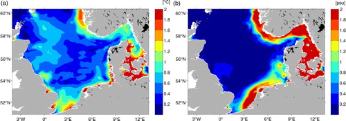
To obtain spatial differences between the global and regional models, we compare the climatological (1950–2000) sea surface temperature (SST; Fig. 2) and sea surface salinity (SSS; Fig. 4) with the climatological data (Janssen et al., 1999). Thereby, we investigate the degree of coherency between the model results and observations on large scales. At the northern boundaries, winter global model temperatures are warmer than observations (Fig. 2 upper panel), which of course similarly influences the regional model. The observation plot displays a 100-yr climatological mean. Hence, the higher temperature in the northern part could be explained by the warm trend recorded over the last 50 yr of the 20th century. However, there is also a clear trend in the shallow southern North Sea in summer (Fig. 2 middle panel), rendering the above explanation questionable. Since there is no 50 yr climatological dataset available, we employ BSH satellite data based on the mean of 22 yr data to compare with modelled results during the same period (1979–2000, Fig. 3). In general, the results are similar to Fig. 2. The northern North Sea in winter in both model results shows higher temperatures than satellite data, which is confirmed to be a model bias. We conclude that the difference between models and observations is introduced by the meteorological forcing. Furthermore, along the British east coast, SST in HAMSOM is closer to observations, which can be explained by the better simulation of the Scottish coastal currents (see Table 1 and Section 3.3).

Fig. 2 Climatological SST (upper panels) and vertical temperature distribution at section 58°N (bottom panels) in February and August of observations (Janssen et al., 1999, left column), MPIOM global (middle column) and HAMSOM regional (right column) simulations. Red lines mark the location of the section at 58°N.

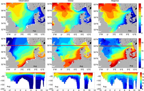
Fig. 3 Mean of 22 yr SST (1979–2000) in February (upper panel) and August (bottom panel) of satellite observations (left column), MPIOM global (middle column) and HAMSOM regional (right column) simulations.

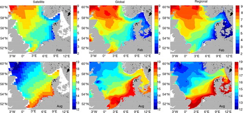
Table 1. Annual mean transport estimations from MPIOM, HAMSOM, HYCOM and measurements

MPIOM	HAMSOM	HYCOM	Data
Orkney-Shetland inflow	0.53	0.57	0.49	0.30
English Channel inflow	0.19	0.08	0.16	0.1–0.17
Norwegian channel outflow	1.49	1.32	2.33	1.8
Shetland shelf inflow	0.73	0.66	0.5	0.6
Skagerrak inflow	0.42	0.81	1.02	0.5–1.5
Skagerrak outflow	0.44	0.84	1.04	0.5–1.5
Eastern British coastal currents	0.01	0.1

The sections are illustrated in Fig. 1. HYCOM results and measurements are taken from Winther and Johannessen (2006) and references therein. All values are given in Sv (1 Sv = 10⁶ m³ s⁻¹).

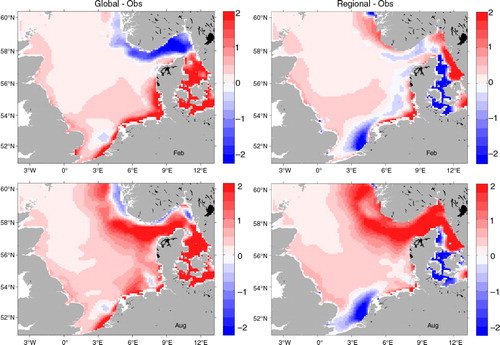
In the MPIOM simulation, the coastal regions exhibit major differences (Fig. 2). The difference in the southern coastal region is also confirmed by the SSS comparison (Fig. 4). Note that in MPIOM a weak salinity restoring (to coarse climatological data) should represent missing sink and source terms. However, it is not adequate in the region close to river mouths. Moreover, the thickness of the first layer is 16 m, which is too coarse to describe the river plume correctly. At the southern boundary, the area influenced by the English Channel inflow, the difference between the MPIOM results and observations is obvious, which could be explained by an overestimated Atlantic inflow through the English Channel in MPIOM (Table 1). The finer resolution HAMSOM results are significantly closer to the observations along the continental coast (both for SST and SSS), indicating that the regional model provides a better representation of near-shore processes. The regions close to open boundaries also exhibit different temperature patterns between the both models. The reason is that HAMSOM only obtains MPIOM results at the open boundary under inflow conditions, and open boundary conditions are applied under outflow conditions.

Fig. 4 Left column: difference between Climatological SSS (psu) in February and August between observations (Janssen et al., 1999) and MPIOM global simulations (MPIOM minus observations). Right column: SSS difference between observations and HAMSOM regional simulations (HAMSOM minus observations).

In order to analyse the effect of specific model features in more detail, we illustrate the vertical temperature distribution at 58°N (Fig. 2, bottom panel). Looking at the observations in summer, the stratification is strong, and the thermocline is at approximately 30 m depth. The stratification in MPIOM is stronger than in HAMSOM, and closer to the observations. The differences can be explained by different vertical resolutions and treatment of the vertical turbulent mixing [MPIOM: Richardson-number dependent formulation by Pacanowski and Philander (1981); HAMSOM employs a scheme uses a level 2 model by Mellor and Yamada (1974)]. Here we demonstrated that a regional focused global model with coarser vertical resolution can well reproduce vertical structure in observations.

The spatial distribution of the root mean square difference (RMSD) of SST between two experiments also shows that the coastal areas exhibit the major difference (Fig. 5a). This is confirmed by the RMSD of SSS (Fig. 5b). Again, the region close to the Rhine Estuary shows major differences, as already mentioned above (a result of SSS restoring to coarse climatological data). The large differences near the Norwegian coast can be explained by the different strength of NCC in the two models (open boundary conditions are applied under outflow conditions).

Fig. 5 Root mean square difference of SST and SSS between MPIOM and HAMSOM model results. (a) RMSD SST; (b) RMSD SSS.

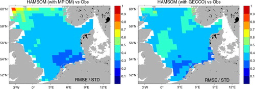
To estimate the impacts of the open boundary data extracted from MPIOM on the HAMSOM results, we compare two HAMSOM runs: one using MPIOM data and one using GECCO data as open boundary values. The ratio of the root mean square error (RMSE) between the model results and the BSH SST data to the standard deviation of BSH SST data is illustrated in Fig. 6. We find that the ratio is higher in the HAMSOM run with MPIOM data along the open boundaries. This can indeed be expected, since GECCO assimilates observational data and hence, results are closer to observations. In the inner model domain, the ratio of both runs is quite similar.

Fig. 6 The ratio of root mean square error (RMSE) to standard deviations of BSH SST data. RMSE is calculated between HAMSOM simulations with open boundary forcing from MPIOM (left) and from GECCO (right) and BSH SST observations (weekly), and only for the years 1979–2000 (data period).

3.2. Seasonal and interannual differences

On the seasonal scale, the major differences between MPIOM results and observations occur in transitional seasons (spring and autumn), while the differences between HAMSOM results and observations (BSH SST data) prominently occur in spring (Fig. 7a). In general, both models are capable of reproducing the mean seasonal observations, but monthly values of interannual variability are smaller than observed (Fig. 7a, error bars). Looking at the interannual scale for both models, the annual mean SST over the entire North Sea is in good agreement with observations with an offset of 0.53°C for MPIOM, and only 0.38°C for HAMSOM (Fig. 7c). This offset can be explained by the parameterisation of the bulk formula in the two models. Possible errors from different meteorological forcing data can be ruled out, since the latter is the same in both models.

Fig. 7 (a) Seasonal cycle of spatially averaged climatological monthly mean SST for the North Sea, error bars denote the standard deviation. (b) Derivative of monthly mean SST (monthly mean SST minus previous monthly mean SST), error bars denote the standard deviation. (c) The inter-annual variability of spatially and yearly averaged SST over the North Sea. Grey and black lines refer to the results from MPIOM and HAMSOM, respectively. The red lines refer to observations.

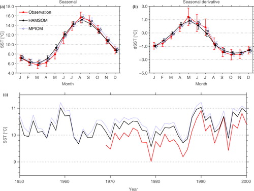
The derivative of the SST (DSST = dSST/dt) is calculated based on monthly data to reflect net heat flux difference between the models and observations. The North Sea averaged DSST seasonal development shows that both models do not produce big differences and agree well with the observations (Fig. 7b). However, they cannot capture the maximum variabilities of DSST in summer (Fig. 7b, error bars). Monthly DSST in a year with a hot summer can reach 6°C/month (not shown), indicating that both models cannot appropriately simulate the induced strong thermal stratification since the model surface layers have a thickness of 5 m or more.

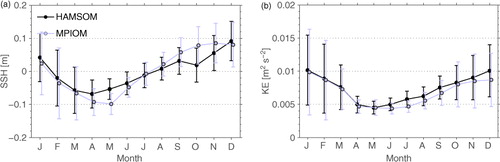
The seasonal cycles of SSH and kinetic energy are displayed in Fig. 8. The kinetic energy is defined as 0.5 (u²+v²), where u and v are monthly depth-averaged horizontal velocity components, thus tidal information is filtered out. The seasonal cycle of kinetic energy (high in winter and low in summer) is affected mainly by winds, while SSH seasonality is a consequence of many factors, including steric effects, wind forcing and external signals from the North Atlantic. Both models show a minimum of kinetic energy in April, but a slightly different timing of the subsequent increase (MPIOM in August, HAMSOM in July, Fig. 8b). The mean seasonality of SSH (Fig. 8a) shows major differences between the two models in spring and autumn, but qualitatively the seasonal cycle is kept (spring low and autumn high). This demonstrates that the seasonal cycle of these two quantities remains stable over long-time integrations.

Fig. 8 Spatially averaged climatological monthly means (lines) and standard deviations (error bars) of SSH (a) and kinetic energy (b). The grey colour refers to the MPIOM results, the black colour to the HAMSOM results.

3.3. Circulation differences between both models

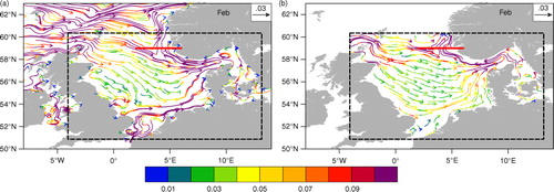
The volume transports in February through different sections are shown in Table 1. The circulation pattern of the northern North Sea is strongly influenced by the Atlantic inflow at the northern entrance. After downscaling, the ESC and NCC outflow both decrease by ~10%, but the circulation in the Skagerrak is stronger in HAMSOM (Table 1). The strong circulation pattern in the Skagerrak is closer to observations and HYCOM results (Winther and Johannessen, 2006), which is probably due to the finer model resolution in this region. We illustrate the surface circulation pattern in February for both models (Fig. 9). Since the first layer thickness is 16 m in MPIOM, for comparison we calculate vertically averaged currents in the upper three layers (15 m) to represent surface currents in HAMSOM. The velocity fields of both models are similar in the northern North Sea. In the southern North Sea, the MPIOM model simulation shows a weak Scottish coastal current, while the inflow from English Channel strongly influences the continental coast (Fig. 9a). In contrast, the HAMSOM model results show a reasonable cyclonic circulation in the southern North Sea and German Bight (Fig. 9b), which is comparable to the previous studies (Pohlmann, 2006; Staneva et al., 2009).

Fig. 9 Climatological surface current fields (m s⁻¹) of (a) MPIOM and (b) HAMSOM (upper 15 m) results for February. The colours refer to current speeds (m s⁻¹). The black dashed line shows the domain of HAMSOM model, and the red thick lines refer to 59°N section in Fig. 10.

To investigate the decadal variability of the currents in different layers, we select a lateral section at 59°N, which covers the northern inflow (Fig. 10, blue shades) as well as the NCC outflow (Fig. 10, red shades) regions. Since the MPIOM boundary values are employed as inflow conditions, inflow rates correlated reasonably (R>0.85, Fig. 10 blue lines) in both models. Outflow conditions, however, are treated differently, using a two-dimensional radiation boundary condition in HAMSOM (Chen et al., 2013). This leads to a narrower outflow in the HAMSOM model results, hence the correlation is substantially weaker at 20 m (R = 0.42, Fig. 10, red lines). However, the correlation is higher at 50 m depth (R = 0.84), since here the baroclinic circulation dominates (see Fig. 2, bottom panel).

Fig. 10 (a, c, e, g) Hovmöller Diagram of meridional current speeds (m s⁻¹) in February at 20 m (upper panel) and 50 m depth (bottom panel) through the 59°N section from 2°E to 6°E (location in Fig. 9) of MPIOM (left panel) and HAMSOM (right panel) model results. Blue indicates the southward, and red indicates the northward current. (b, d, f, h) The blue and red solid lines refer to the simple sum of the current speeds across the section, respectively. The correlation coefficients between both model results at 20 m depth are R = 0.87 (southward current) and R = 0.42 (northward current), and at 50 m depth are R = 0.94 (southward current), R = 0.84 (northward current). The mean north- and southward currents are presented by the dashed lines with their values (m s⁻¹) noted at the x-axis of b, d, f, h.

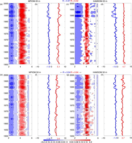
On average, the mean southward inflow in winter decreases by 15% at 20 m in the course of nesting (Fig. 10b and 10d blue dotted lines), whereas the NCC outflow decreases by 8% at 20 m, but retains the same magnitude at 50 m (Fig. 10b, 10d, 10f, and 10h, red dotted lines). Therefore, we infer that the decrease of transport across the northern boundary (~10%) occurs mainly in the upper 50 m.

4. Discussion

By comparison, we found that the stretched global model reproduced similar features as the conventional nested regional model although it has a coarser vertical resolution. The advantage of the absence of open lateral boundaries in the global model can be demonstrated, in particular for the transition region between the North Sea and Baltic Sea. An increase of computer time by factor 2 is acceptable. In brief, the differences between the results of the both models are on the one hand definitely influenced by open boundary conditions, the locations of open boundaries and on the other hand by the specific model characteristics. The differences in model architecture contribute mainly to deviations in temperature and salinity in coastal regions (thus also to the coastal baroclinic circulation), while circulation changes throughout the North Sea can be explained by the open boundary conditions under outflow conditions in the regional model. As expected, the regional model introduces more spatial variability into the North Sea system, which in turn also affects the outflow variability, while the magnitude of the mean outflow is nearly unchanged (Fig. 10).

Whether the pathways of the North Atlantic Current (NAC) into the North Sea will change in future is one of the key questions in regional climate research (Winther and Johannessen, 2006), which also crucially impacts the circulation in the North Sea (Albretsen and Røed, 2010). A faithful representation of the pathways is a prerequisite for North Sea downscaling of global simulations. In general, coarse resolution global models cannot capture the current along the Norwegian Trench very accurately, because the horizontal resolution is usually not sufficient to represent the related dynamics. In our downscaling experiments, the ESC and NCC both decrease by ~10%, in contrast to the conclusion of Ådlandsvik and Bentsen (2007). This is probably caused by the fact that the northern boundary in our model is further south than in Ådlandsvik and Bentsen (2007), and it is shown that nesting experiments with different locations of open boundaries could produce different results. We also find that the correlation of the NCC between both models is weak at the surface but strong at 50 m depth (Fig. 10). We hypothesise that the different amount of freshwater discharge along the Norwegian coast into NCC in the two models contributes to the weak correlation at the surface. Altogether, the results confirm that zooming experiment can reasonably reproduce the general pathways, and could be used as an ocean component in a free climate model.

The regional downscaling provides additional spatial and temporal details to the global simulation. In order to deal with the often unreasonable boundary conditions provided by global models, bias correction methods are frequently applied (e.g. Katzfey et al., 2009; Mathis, 2013). Normally, the bias correction assures that the same statistical characteristics are kept as the observational references, but it introduces more uncertainty to the system. In this study, we have shown that the stretched global model can well depict the large scale features of the high-resolution regional model and produce reasonable results on a decadal time scale.

5. Summary

In this study, the ocean component of a regional climate model system has been evaluated. This ocean component includes a stretched global model and a well validated regional shelf model. By evaluating the hindcast experiments performed with the two models, we obtain insight into the question whether the decadal variability could correctly propagate from the global to the regional scale.

On the climatological scale, the SST differences between the two experiments are not significant, but major differences occur for SSS. The higher SSS in coastal water obtained in the global model pinpoints the general limitation of the global model, by underestimating coastal processes. The different vertical structures (stratification) which have been simulated show the effect of the different turbulent schemes implemented in the two models.

On the seasonal scale, the major SST differences between the models and observations occur in the transitional months (up to 2°C in spring, up to 1°C in autumn). The regional model results exhibit a similar SST bias during the spring period, but not in autumn. Furthermore, the seasonal cycles of SSH and kinetic energy are similar, indicating the robust seasonality of these quantities.

Interannually, the SST of both models shows a constant bias of ~0.3°C compared to observations. The climatological velocity fields of both model simulations are similar. In the nesting experiment, the NAC inflow through the northern entrance decreases by ~10%, but the circulation in the Skagerrak is stronger in HAMSOM.

Moreover, we examined the RMSD of SST and SSS between the two model results to examine their horizontal distribution. The RMSD for SST reaches up to 2°C in coastal regions. The RMSD of SSS reflects the effect of different treatment of the models with respect to river discharge, which could be amplified in long-time simulations.

To conclude, the stretched global model can well depict the large scale features of the high-resolution regional model, while the disadvantage is a poorer representation in coastal regions. Although open boundary conditions are applied, the regional model results demonstrate that the decadal variability can be transferred to the North Sea system properly without the necessity to employ a bias correction. Hence, we suggest that the stretched global model system can be a suitable tool for long-term free climate model simulations, and the only limitation is in the coastal region. Regarding the coastal region focused studies (e.g. in the Wadden Sea), nested regional model can considerably improve the results. For both schemes, we provide a quality assurance of the system by comparing the large and local scale information.

6. Acknowledgement

This work was performed in the frame of the BMVBS project KLIWAS (Impacts of climate change on waterways and navigation – Searching for options of adaptation). We are grateful to the anonymous reviewer for the constructive comments, which improved the manuscript.

References

- Ådlandsvik B. , Bentsen M . Downscaling a twentieth century global climate simulation to the North Sea. Ocean. Dyn. 2007; 57(4): 453–466.
- Albretsen J. , Røed L. P . Decadal long simulations of mesoscale structures in the northern North Sea/Skagerrak using two ocean models. Ocean Dyn. 2010; 60(4): 933–955.
- Aldrian E. , Sein D. , Jacob D. , Gates L. D. , Podzun R . Modelling Indonesian rainfall with a coupled regional model. Clim. Dyn. 2005; 25(1): 1–17.
- Backhaus J. O . A three-dimensional model for the simulation of shelf sea dynamics. Dtsch. Hydrographische Z. 1985; 38: 165–187.
- Chen X. , Liu C. , O'Driscoll K. , Mayer B. , Su J. , co-authors . On the nudging terms at open boundaries in regional ocean models. Ocean Model. 2013; 66: 14–25.
- Damm P. E . The seasonal salinity and freshwater distribution in the North Sea and its balance. 1997; Institute of Oceanography, Hamburg, Germany. Vol. 28.
- Dooley H. D . Hypotheses concerning the circulation of the northern North Sea. ICES J. Mar. Sci. 1974; 36(1): 54–61.
- Fox-Rabinovitz M. , Côté J. , Dugas B. , Déqué M. , McGregor J. L . Variable resolution general circulation models: stretched-grid model intercomparison project (SGMIP). J. Geophys. Res. Atmos. 2006; 111: D16104.
- Fox-Rabinovitz M. , Cote J. , Dugas B. , Deque M. , McGregor J. L. , co-authors . Stretched-grid model intercomparison project: decadal regional climate simulations with enhanced variable and uniform-resolution GCMs. Meteorol. Atmos. Phys. 2008; 100(1–4): 159–178.
- Griffies S. M. , Böning C. , Bryan F. O. , Chassignet E. P. , Gerdes R. , co-authors . Developments in ocean climate modelling. Ocean Model. 2000; 2(3): 123–192.
- Gröger M. , Maier-Reimer E. , Mikolajewicz U. , Moll A. , Sein D . NW European shelf under climate warming: implications for open ocean–shelf exchange, primary production, and carbon absorption. Biogeosciences. 2013; 10(6): 3767–3792.
- Gurgel K.-W. , Dzvonkovskaya A. , Pohlmann T. , Schlick T. , Gill E . Simulation and detection of tsunami signatures in ocean surface currents measured by HF radar. Ocean Dyn. 2011; 61(10): 1495–1507.
- Holt J. , Wakelin S. , Lowe J. , Tinker J . The potential impacts of climate change on the hydrography of the northwest European continental shelf. Prog. Oceanogr. 2010; 86(3): 361–379.
- Hurrell J . Decadal trends in the North Atlantic Oscillation: regional temperatures and precipitation. Science. 1995; 269(5224): 676–679.
- IPCC. Climate change 2007. The physical science basis. Contribution of Working Group I to the Fourth Assessment Report of the Intergovernmental Panel on Climate Change. 2007; Cambridge, United Kingdom: Cambridge University Press.
- Janssen F. , Schrum C. , Backhaus J . A climatological data set of temperature and salinity for the Baltic Sea and the North Sea. Dtsch. Hydrographische Z. 1999; 51: 5–245.
- Janssen F. , Schrum C. , Hubner U. , Backhaus J . Uncertainty analysis of a decadal simulation with a regional ocean model for the North Sea and Baltic Sea. Clim. Res. 2001; 18(1/2): 55–62.
- Jungclaus J. H. , Fischer N. , Haak H. , Lohmann K. , Marotzke J. , co-authors . Characteristics of the ocean simulations in the Max Planck Institute Ocean Model (MPIOM) the ocean component of the MPI-Earth system model. J. Adv. Model. Earth Syst. 2013; 5(2): 442–446.
- Kalnay E. , Kanamitsu M. , Kistler R. , Collins W. , Deaven D. , co-authors . The ncep/ncar 40-year reanalysis project. Bull. Am. Meteorol. Soc. 1996; 77(3): 437–471.
- Katzfey J. , McGregor J. , Nguyen K. , Thatcher M . Anderssen R. S. , Braddock R. D. , Newham L. T. H . Dynamical downscaling techniques: impacts on regional climate change signals. 18th World IMACS congress and MODSIM09 international congress on modelling and simulation. 2009; 2377–2383. Modelling and Simulation Society of Australia and New Zealand and International Association for Mathematics and Computers in Simulation, Vol. 13.
- Köhl A. , Stammer D . Decadal sea level changes in the 50-year GECCO ocean synthesis. J. Clim. 2008; 21(9): 1876–1890.
- Levitus S. , Boyer T. P. , Antonov J . World ocean atlas 1994. Volume 5. Interannual variability of upper ocean thermal structure. 1994; PB–95-270120/XAB, National Environmental Satellite, Data, and Information Service, Washington, DC, USA: Technical report.
- Marchesiello P. , McWilliams J. C. , Shchepetkin A . Open boundary conditions for long-term integration of regional oceanic modelsm. Ocean Model. 2001; 3(1–2): 1–20.
- Marsland S. , Bindoff N. , Williams G. , Budd W . Modeling water mass formation in the Mertz Glacier Polynya and Adélie Depression, east Antarctica. J. Geophys. Res. 2004; 109(C11): C11003.
- Marsland S. , Haak H. , Jungclaus J. , Latif M. , Roske F . The Max-Planck-Institute global ocean/sea ice model with orthogonal curvilinear coordinates. Ocean Model. 2003; 5(2): 91–127.
- Mathis M . Projected Forecast of Hydrodynamic Conditions in the North Sea for the 21st Century. 2013; University of Hamburg: Doctoral Thesis.
- Mathis M. , Mayer B. , Pohlmann T . An uncoupled dynamical downscaling for the North Sea: method and evaluation. Ocean Model. 2013; 72: 153–166.
- Mayer B. , Damm P. , Pohlmann T. , Rizal S . What is driving the ITF? An illumination of the Indonesian throughflow with a numerical nested model system. Dyn. Atmos. Ocean. 2010; 50(2): 301–312.
- McGregor J. L . Recent developments in variable-resolution global climate modelling. Clim. Change. 2013; 119
- Meier H . Regional ocean climate simulations with a 3D ice-ocean model for the Baltic Sea. Part 1: model experiments and results for temperature and salinity. Clim. Dyn. 2002; 19(3–4): 237–253.
- Meier H. E. , Kauker F . Modeling decadal variability of the Baltic Sea: 2. Role of freshwater inflow and large-scale atmospheric circulation for salinity. J. Geophys. Res. Oceans. 2003; 108(C11): 3368.
- Mellor G. L. , Yamada T . A hierarchy of turbulence closure models for planetary boundary layers. J. Atmos. Sci. 1974; 31(7): 1791–1806.
- Meyer E. M. , Pohlmann T. , Weisse R . Thermodynamic variability and change in the North Sea (1948–2007) derived from a multidecadal hindcast. J. Mar. Syst. 2011; 86(3–4): 35–44.
- Mikolajewicz U. , Sein D. V. , Jacob D. , Königk T. , Podzun R. , co-authors . Simulating Arctic sea ice variability with a coupled regional atmosphere-ocean-sea ice model. Meteorol. Z. 2005; 14(6): 793–800.
- O'Driscoll K. , Mayer B. , Ilyina T. , Pohlmann T . Modelling the cycling of persistent organic pollutants (POPs) in the North Sea system: fluxes, loading, seasonality, trends. J. Mar. Syst. 2013; 111–112: 69–82.
- Pacanowski R. , Philander S . Parameterization of vertical mixing in numerical models of tropical oceans. J. Phys. Oceanogr. 1981; 11(11): 1443–1451.
- Palma E. D. , Matano R. P . On the implementation of passive open boundary conditions for a general circulation model: the barotropic mode. J. Geophys. Res. 1998; 103: 1319–1341.
- Pohlmann T . Predicting the thermocline in a circulation model of the North Sea. 1. Model description, calibration and verification. Cont. Shelf Res. 1996; 16(2): 131–146.
- Pohlmann T . A meso-scale model of the central and southern North Sea: consequences of an improved resolution. Cont. Shelf Res. 2006; 26(19): 2367–2385.
- Rodhe J . On the dynamics of the large-scale circulation of the Skagerrak. J. Sea Res. 1996; 35(1): 9–21.
- Schrum C . Regionalization of climate change for the North Sea and Baltic Sea. Clim. Res. 2001; 18(1–2): 31–37.
- Schrum C. , Hübner U. , Jacob D. , Podzun R . A coupled atmosphere/ice/ocean model for the North Sea and the Baltic Sea. Clim. Dyn. 2003; 21(2): 131–151.
- Staneva J. , Stanev E. , Wolff J.-O. , Badewien T. , Reuter R. , co-authors . Hydrodynamics and sediment dynamics in the German Bight. A focus on observations and numerical modelling in the east Frisian Wadden Sea. Cont. Shelf Res. 2009; 29(1): 302–319.
- Su J. , Pohlmann T . Wind and topography influence on an upwelling system at the eastern Hainan coast. J. Geophys. Res. 2009; 114(C6): C06017.
- Svendsen E. , Sætre R. , Mork M . Features of the northern North Sea circulation. Cont. Shelf Res. 1991; 11(5): 493–508.
- Thomas M. , Sündermann J. , Maier-Reimer E . Consideration of ocean tides in an OGCM and impacts on subseasonal to decadal polar motion excitation. Geophys. Res. Lett. 2001; 28(12): 2457–2460.
- Turrell W. R. , Henderson E. W. , Slesser G. , Payne R. , Adams R. D . Seasonal changes in the circulation of the northern North Sea. Cont. Shelf Res. 1992; 12(2): 257–286.
- Weisse R. , von Storch H. , Callies U. , Chrastansky A. , Feser F. , co-authors . Regional meteorological-marine reanalyses and climate change projections: results for Northern Europe and potential for coastal and offshore applications. Bull. Am. Meteorol. Soc. 2009; 90(6): 849–860.
- Winther N. G. , Johannessen J. A . North Sea circulation: Atlantic inflow and its destination. J. Geophys. Res. Oceans. 2006; 111(C12): C12018.