Impact of partly ice-free Lake Ladoga on temperature and cloudiness in an anticyclonic winter situation – a case study using a limited area model

Abstract

At the end of January 2012, a low-level cloud from partly ice-free Lake Ladoga caused very variable 2-m temperatures in Eastern Finland. The sensitivity of the High Resolution Limited Area Model (HIRLAM) to the lake surface conditions was tested in this winter anticyclonic situation. The lake appeared to be (incorrectly) totally covered by ice when the lake surface was described with its climatology. Both parametrisation of the lake surface state by using a lake model integrated to the NWP system and objective analysis based on satellite observations independently resulted in a correct description of the partly ice-free Lake Ladoga. In these cases, HIRLAM model forecasts were able to predict cloud formation and its movement as well as 2-m temperature variations in a realistic way. Three main conclusions were drawn. First, HIRLAM could predict the effect of Lake Ladoga on local weather, when the lake surface state was known. Second, the current parametrisation methods of air–surface interactions led to a reliable result in conditions where the different physical processes (local surface processes, radiation and turbulence) were not strong, but their combined effect was important. Third, these results encourage work for a better description of the lake surface state in NWP models by fully utilising satellite observations, combined with advanced lake parametrisation and data assimilation methods.

• lake-effect
• data assimilation
• lake ice
• NWP
• cold outbreaks
• stable boundary layer
• lake–atmosphere interaction

1. Introduction

At the end of January 2012, a local newspaper ‘Etelä-Saimaa’, published in Southeastern Finland (in Finnish), reported on an outstanding weather phenomenon. During a couple of days, the air temperature had been varying by as much as 17°C within a small area. For instance, in Imatra a temperature of −11°C was observed, while in Parikkala (60 km northeast of Imatra), the temperature at the same time was −28°C. According to the duty meteorologist of the Finnish Meteorological Institute interviewed by the newspaper, the large variability was due to a low cloud, which originated from partly ice-free Lake Ladoga. It was predicted that this situation would not last very long, because Lake Ladoga was about to freeze. The newspaper noted that Lake Ladoga, which is the largest lake in Europe (17 700 km², located in Russia between 30°E–35°E and 60°N–62°N) influences the weather of Eastern Finland because it is large and so close. What made the phenomenon interesting was that the low-level cloud, spread by the wind, only covered a small area at a given time. This created the large and at that time unpredicted variability in the observed temperature both in space and time.

We used this winter case to study the sensitivity of a Numerical Weather Prediction (NWP) model to the description of the lake surface state. The purpose of this work was to study the impact of partly ice-free Lake Ladoga on cloudiness and temperature in a winter anticyclonic situation and to answer the question: can a NWP model predict correctly the evolution of clouds and the consequent large 2-m temperature variability, if it is provided with a correct description of the lake surface state? As the NWP model, we used the High Resolution Limited Area Model (HIRLAM, Undén et al., 2002; Eerola, 2013), where different possibilities to handle the air–lake interactions were available. In this kind of situation, the balance between different surface-related processes is subtle. Thus this case provided a good test-bench for the model.

At the northern and middle latitudes, lakes regularly freeze during the winter. However, due to their large heat capacity they often stay ice-free late in the autumn and early winter. Their influence on local weather depends on the synoptic situation and on the lake surface conditions (open water, partly or totally ice-covered). Heavy snowstorms caused by the ice-free lakes are well documented, especially for the North American Great Lakes area (e.g. Niziol et al., 1995; Vavrus et al., 2013; Wright et al., 2013). Cordeira and Laird (2008) even documented two cases, where snowstorms developed over a lake mostly covered by ice. The authors stated that despite of the decreased turbulent fluxes from the surface, a variety of ice-cover conditions and meso- and synoptic-scale factors supported the development of snowstorms. Based on earlier studies, Niziol et al. (1995) listed several factors, which have been noticed to be important in the evolution of lake-induced snowfall in this area, the most important being the air–lake temperature difference. Other influencing factors included the cloud-top inversion height and strength, the differences in temperature and surface roughness between the lake and surrounding land surfaces, as well as the orographic lift downwind of the lake. In Scandinavia, Andersson and Nilsson (1990), Andersson and Gustafsson (1994), and Gustafsson et al. (1998) discussed the influence of the Baltic Sea, whose size is comparable to that of the Great Lakes, on convective snowfall over the ice-free water surface. According to these authors, favourable factors for the development of precipitating convective cloud bands are the ice-free conditions, suitable topography on the upwind and downwind coasts, a large temperature difference between water and air, and an optimal wind direction which allows for the longest fetch.

Skilful forecasters in Finland know by experience that Lake Ladoga or even smaller lakes may enhance snowfall in autumn or early winter. However, to the authors’ knowledge, there are no documented cases where lakes would have caused heavy snowstorms at the Scandinavian high latitudes. One possible explanation is the small probability for the outbreaks of very cold air during autumn, when large lakes are still warm enough. Lakes in the Scandinavian–Karelian region are numerous but small and often shallow, with rather flat topography around them. Later in winter most of them freeze quickly due to their small size and shallowness. Because of this, the air–lake temperature differences remain moderate.

Meteorologically the case described in the newspaper differed from the severe snowstorm cases. This was a stable anticyclonic situation, with high surface pressure, cold clear-sky winter weather, weak winds and a sharp surface-based temperature inversion. Only light snowfall was detected. However, over ice-free water a large temperature difference between the air and lake prevailed. In a cold winter-time anticyclonic situation, the near-surface air temperature is largely controlled by the cloud cover. In this case, the partly ice-free Lake Ladoga generated a low-level cloud, which spread far into Eastern Finland. Locally, under the cloud cover, temperature rose but under the clear sky it remained low. Such synoptic cases have not been popular in the scientific literature. As a synthesis, based on existing lake-effect literature, Laird et al. (2003) showed a general picture of favourable situations for different lake-effect phenomena as a function of wind speed and air–water temperature difference. Widespread cloud coverage requires strong surface wind and a large enough air–water temperature difference. In weak-wind situations, like this case, shoreline cloud bands can occur. In cases where the air–water temperature difference exceeds 10°C in weak-wind situations, even mesoscale vortex events have been observed.

HIRLAM (Undén et al., 2002; Eerola, 2013) has recently been used in several studies with the aim of improving the treatment of lakes and their influence on local weather. The Freshwater Lake model FLake (Mironov, 2008; Mironov et al., 2012) was implemented into HIRLAM by Kourzeneva et al. (2008) in order to predict lake temperature as well as the evolution of lake ice and its snow cover. From the analysis side, interpolation of in-situ and remote sensing observations of Lake Surface Water Temperature (LSWT) into HIRLAM has been applied by Eerola et al. (2010), Rontu et al. (2012), and Kheyrollah Pour et al. (2014b). In this study, we present and discuss results from three HIRLAM experiments where the state of lakes was described in different ways. The first experiment relied on climatological lake surface conditions according to a method still applied in many large-scale operational NWP systems. In the second experiment, the prognostic lake parametrisation by FLake was used to predict the evolving state of the lake during the atmospheric forecast. In the third experiment, satellite observations were used for the analysis of LSWT and the diagnosis of lake ice concentration (LIC). During the forecast they were kept unchanged.

A standard verification of the NWP results against regular weather observations is sometimes insufficient to show the benefits of model improvements. This is because such a validation collects statistics from a large variety of situations so that the different effects become hidden behind the averages. A careful analysis of well-chosen cases can provide more information about the physical processes and their interactions. Here we report a case study in a situation where the extreme cloud and temperature variations lasted only a couple of days and the influence of Lake Ladoga extended only to Eastern Finland. We focus on the most striking 24-hour period, when a low-level cloud moved across the domain. Because the influence of lakes (even large lakes) on weather and climate is local, depending on local conditions and the weather parameter in question, we restrict ourselves to the closest observations around Lake Ladoga. In addition, we present results of statistical validation against observations during 2 weeks of the prevailing anticyclonic weather in January–February 2012.

This paper is structured as follows: After this introduction, the weather situation is described in Section 2. Special attention is paid to the cloud and temperature variability. Section 3 describes the HIRLAM NWP system, focusing on the surface-related parametrisations and surface data analysis. Also the setup of the three different experiments is described. The results are presented and discussed in Section 4. The movement of the lake-originated cloud and its influence on temperature is described. The surface energy balance is analysed over open water and snow-covered land. In addition, statistical verification results in the vicinity of the lake are shown and discussed. Finally, the results are summarised in Section 5.

2. Weather situation

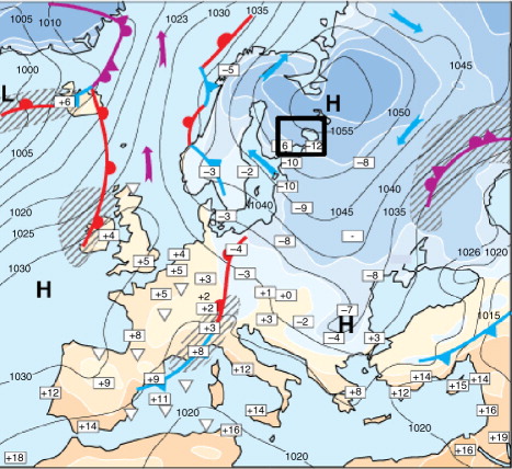
During the last week of January and first week of February 2012, a strong anticyclone extended from Russia to Finland. Figure 1 shows the weather situation in Europe on 28 January. In Eastern Finland, the highest measured mean sea level pressure in 40 yr, 1063 hPa, was recorded during this period. A cold continental winter-time air mass prevailed, with 850 hPa level temperatures between −10 and −15°C in the last week of January and decreasing below −20°C during the first week of February. Typically, this kind of anticyclonic situation is characterised by clear-sky conditions, weak wind, strong and sharp surface-based inversion in temperature, and low 2-m temperatures. Especially in Eastern Finland, very cold temperatures were recorded, with a minimum of −37.5°C at Konnunsuo (WMO station number 02733) on 5 February.

Fig. 1 General weather situation in Europe on 28 January 2012 12 UTC. Mean sea level pressure (contours) and 2-m temperature (shaded) are based on ECMWF analysis. The boxes show selected observed temperatures. The black rectangle box shows the area of interest of this study. (Source: Finnish Meteorological Institute)

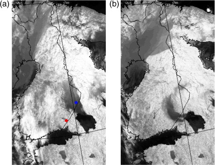
In this case, temperature and cloudiness in Eastern Finland were very variable both in time and space, illustrated by the example in Fig. 2, which shows 2-m temperatures at the Konnunsuo (02733) and Tohmajärvi (02832) stations for the period from 24 January to 5 February. Their locations are marked in Fig. 3 with red and blue dots, respectively. Tohmajärvi is situated about 150 km northeast of Konnunsuo. On top of the diurnal cycle, with an amplitude of approximately 10°C, caused by solar radiation, there were remarkable irregularities. At the more northern station Tohmajärvi, the regular diurnal cycle was disturbed during the night of 28 January, having very small night-time cooling. In the evening on 28 January and the following night the temperature dropped by about 16°C and remained low until the end of the period. At the more southern station Konnunsuo a rapid warming of 15°C took place in the daytime on 29 January. Here the warmer period lasted several days, except for the night of 29 January, before the temperature dropped again on 1 February. The temperature drop between 31 January and 1 February was 21°C, from −11°C to −32°C. The reason for the irregular temperature variations was the changing cloudiness. During 28–29 January, the low-level cloud deck of a length of ca. 200 km and a width of 50–100 km, originating from the ice-free northern part of Lake Ladoga, moved from north to south over Southeastern Finland, as shown in Fig. 3. The clouds caused a rise of temperature first in the north (e.g. at the station Tohmajärvi), while by morning of 29 January the cloud had moved southwards, affecting the temperature there (e.g. at Konnunsuo). Based on observations and a series of satellite images acquired between 29 and 31 January (not shown), the cloud moved so that it affected the temperature only at Konnunsuo, while at Tohmajärvi the temperature kept the regular diurnal cycle with an amplitude of about 10°C. On the first days of February, the cloud occasionally affected the temperature at Konnunsuo. For instance, on 3 February the warm night temperature followed by quick cooling in the afternoon can be explained by changes in the cloud cover.

Fig. 2 Observed 2-m temperature at two stations, Konnunsuo (02733) and Tohmajärvi (02832) in Eastern Finland from 24 January to 5 February 2012. The distance between stations is about 150 km.

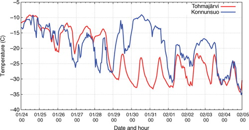
Fig. 3 NOAA AVHRR thermal IR images over Finland and Karelia on 28 January 06 UTC (a) and on 29 January 00 UTC (b) 2012. The low-level cloud cover, shown with dark-grey shades, spreads first northward (a) and later westward (b) from Lake Ladoga. In the single-channel images, the cloud over Lake Ladoga cannot be distinguished from the dark water surfaces. The stations Konnunsuo and Tohmajärvi, referred to in Fig. 2, are marked with red and blue dots, respectively.

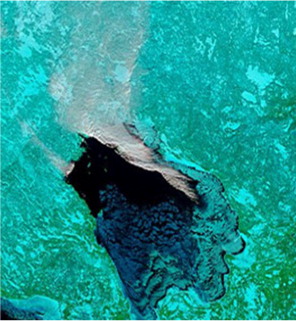
The cloud developed over Lake Ladoga because the lake was still partly ice-free. Compared to the nearby lakes, Lake Ladoga is very large and deep, with maximum and mean depths of 222 m and 52 m, respectively. The northern parts are the deepest while the southern parts are relatively shallow. Lake Ladoga remains free of ice until early winter, when all other nearby lakes are already frozen. This was the case also at the end of January 2012. The northern parts of the lake were open but the shallow southern parts were covered by fractional ice, as seen in the Moderate Resolution Imaging Spectrometer (MODIS)/Terra satellite image (Fig. 4) on 28 January. A sequence of satellite images reveals that freezing advanced gradually in the cold air mass until the whole lake was completely frozen around 6 February (not shown). This was later than on average – in some years the freezing of Lake Ladoga already begins during the second half of December.

Fig. 4 MODIS-Terra colour composite image over Lake Ladoga on 28 January 2012 9:20 UTC. The dark colour in the northern part of the lake shows the ice-free part. South of it, an area of fractional ice can be seen. The white plume of the low-level cloud cover on the northeastern part of the lake is spreading northward.

3. The model and methodology

The HIRLAM NWP system used in this study comprises an upper air and surface data assimilation system, a forecast model with a comprehensive set of physical parametrisations, and methods for pre- and post-processing observations and forecasts (Undén et al., 2002; Eerola, 2013). This study was based on the latest reference HIRLAM (version 7.4, released in March 2012). In that version the freshwater lake parametrisation based on FLake (Mironov, 2008; Mironov et al., 2012) may be applied for prediction of lake variables. For the atmospheric data assimilation, we used for simplicity the three-dimensional variational method (3DVAR) instead of the default four-dimensional variational analysis (4DVAR). We describe here briefly surface data assimilation and the parametrisation of atmospheric and surface processes relevant to this study.

The method of optimal interpolation [OI, e.g. Daley (1991)] is used for the analysis of LSWT and sea surface temperature (SST) at initial time of each forecast. LIC and sea ice concentration (SIC) are traditionally treated together with LSWT and SST using simple relations to convert from one to another (Rontu et al., 2012; Kheyrollah Pour et al., 2014b). For the current study, LSWT and LIC are of special interest. Only few conventional observations of LSWT are available regularly, so climatological information on LSWT/LIC is traditionally used in NWP models. Early versions of HIRLAM used this climatological information in the form of ‘pseudo observations’ (Rontu et al., 2012). Technically, the possibility of using satellite or any other extra observations of LSWT/LIC is available for numerical experiments. In the case when FLake is not applied, the background for the LSWT analysis is provided by the previous analysis, relaxed to climatology. If FLake is applied, LSWT from its short forecast is used as the background. However, the analysed LSWT does not directly influence the next forecast of the lake variables by FLake as this would require development and application of more advanced data assimilation methods (Rontu et al., 2012; Kheyrollah Pour et al., 2014b).

The HIRLAM surface scheme is based on the method of mosaic tiles (Avissar and Pielke, 1989). Each surface type is handled independently and the tiles affect each other only through the atmosphere. The total vertical turbulent and radiative fluxes in a grid square are obtained as weighted averages of fluxes over different surface types. Five surface types are defined: water, ice, bare land, forest, and agricultural terrain/low vegetation. The water and ice tiles may consist of sea or lake. For the three land surface types and sea ice, prognostic parametrisation is based on a two-layer ISBA scheme (Interactions between Surface–Biosphere–Atmosphere) (Noilhan and Planton, 1989; Noilhan and Mahfouf, 1996), modified according to Gollvik and Samuelsson (2010) to improve interactions related to forest, snow, and ice.

Over land and ice the surface temperature is determined by the surface energy balance consisting of net radiation fluxes, heat flux from the underlying surface, and turbulent fluxes at the surface. Over sea, SST and ice cover given by the surface analysis are kept constant during the forecast and the ice surface temperature is predicted using a simple thermodynamic parametrisation based on Gollvik and Samuelsson (2010). Over lakes, LSWT and LIC are treated in a similar way if the FLake parametrisation is not applied (experiments OLD and NHA described below). If FLake is used (experiment TRU), the mean lake water, ice, and snow temperatures as well as the lake ice depth are prognostic variables. At every time step, the lake surface temperature, which interacts with the atmosphere, is diagnosed from the uppermost predicted temperature (snow, ice or water).

The turbulent heat and momentum fluxes are treated separately in the surface layer (the lowest model layer) and above it. In the surface layer, stability functions by Louis (1979) and predefined roughness values are applied for calculation of the fluxes over each surface type, with own prognostic surface temperature and moisture. Above the surface layer, a scheme based on turbulent kinetic energy approach (Cuxart et al., 2000) is applied, using the grid-averaged surface fluxes as the lower boundary condition.

The weather parameters discussed in this study are the screen-level (or 2-m) air temperature and the fractional low-level cloud cover. In HIRLAM, the screen-level temperature is estimated from the predicted temperature on the lowest model level (about 12 m above the surface) and the surface temperature, taking into account the surface layer stability. It is calculated separately for each surface type in a gridbox and the grid-scale value is obtained as an area-weighted average. The surface temperatures in the tiles are very sensitive to the radiative and heat transfer properties of the surface, which may be completely different for land, water, ice, and snow. In the current meteorological situation, the long-wave radiation (LWD) was crucial for the evolution of the screen-level temperature. The net LWD flux at the surface depends on the surface temperature and on the LWD emitted by the (moist) air and clouds towards the surface. The basic prognostic variables, affecting the cloud–radiation interactions in HIRLAM, are the in-cloud specific liquid water and ice content as well as the air temperature and humidity at the level of clouds. The three-dimensional diagnostic cloud fraction is derived from the relative humidity (Sundqvist et al., 1989; Sundqvist, 1993). The amount of low clouds is defined by taking the maximum total cloud cover from all levels from the surface to the level of about 750 hPa or about 2500 m. Details of the radiation, cloud and turbulence parametrisations applied in HIRLAM can be found in Undén et al. (2002).

For this study we defined three HIRLAM experiments: OLD, TRU, and NHA, which differed from each other only in the way how lake surface state was described. The first experiment OLD represented a traditional large-scale NWP system, where LSWT and LIC were determined by their climatological values. This was achieved by picking up LSWT values from the ECMWF analyses to be used as observations in the surface analysis (Eerola et al., 2010). Over selected large lakes, including Lake Ladoga, these analyses contained LSWT estimated from time-lagged simulated screen-level temperatures (G-P. Balsamo, personal communication). LIC was derived diagnostically from LSWT, as discussed earlier. LSWT and LIC were kept unchanged during the forecasts.

The second experiment TRU used the prognostic lake parametrisation by FLake. No observations on or close to Lake Ladoga were introduced into the LSWT analysis. Thus the lake surface state was totally determined by FLake. This experiment was similar to TRULAK in Kheyrollah Pour et al. (2014b). In the third experiment NHA, satellite data from the MODIS, operating on NASA's Terra and Aqua satellites were used (Kheyrollah Pour et al., 2014a, b). MODIS observations were introduced at 15 pre-selected locations over Lake Ladoga as in the experiment NHALAK in Kheyrollah Pour et al. (2014b).

The experiments were run independently of each other. Experiment TRU was run through the whole winter 2011–2012 and experiment NHA from the beginning of January 2012 to the end of May 2012. Experiment OLD was run for a shorter period containing the second half of January 2012. Four data assimilation-forecast cycles per day were initiated at 00, 06, 12 and, 18 UTC, but longer forecasts of 27 hours lead time started only from analyses at 00 and 12 UTC. The experiments were run over a Nordic domain shown on the upper right corner of Fig. 5a, using a horizontal resolution of ca. 7.5 km and 65 levels in vertical. The density of levels was highest in the boundary layer: 20 levels were used within the lowest one km. Lateral boundary conditions of the atmospheric variables were provided by the ECMWF analyses.

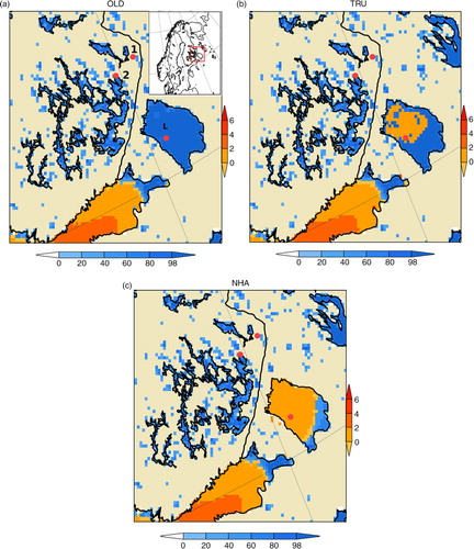
Fig. 5 Simulated ice concentration (%, scale at bottom) and surface water temperature (°C, scale on the right) on 28 January 00 UTC from the three experiments: OLD (a), TRU (b), and NHA (c). The red dots marked with 1 and 2 in (a) show the two observation stations: 1=Ilomantsi, 2=Joensuu (discussed in Sections 4.2 and 4.3). Point L over Lake Ladoga shows the gridpoint discussed in Section 4.3. The embedded small map in (a) shows the whole integration area of the experiments and the red rectangle box the area of interest of this study.

4. Results and discussion

We analysed, evaluated and validated results of the three HIRLAM experiments between 25 January and 5 February, discussing in detail the results for one 27-hour forecast starting from the analysis at 28 January 00 UTC. This short (1 d) period was challenging to the HIRLAM model, and would be as difficult to any other NWP model, because of the quick changes in local cloud cover and 2-m temperature. The predicted synoptic-scale features, such as location and strength of the anticyclone, were similar in all experiments. Therefore, the contrasting weather forecasts for Eastern Finland by the experiments were due to the differently simulated description of the state of Lake Ladoga.

4.1. Simulated ice concentration on Lake Ladoga

Figure 5 shows LSWT and LIC according to the three experiments at 00 UTC on 28 January, i.e. at the initial (analysis) time of the forecasts in question. In OLD, Lake Ladoga was completely frozen, according to the climatology. In TRU and NHA, the northern part of the lake was ice-free as in reality (Fig. 4). In TRU, the lake model FLake predicted the northern parts of Lake Ladoga as ice-free. In NHA, the satellite observations used in the analysis allowed to describe most of the lake as ice-free. None of the experiments could describe well the area of fractional ice seen in Fig. 4 over the southern part of Lake Ladoga. In NHA, the simple relations for the diagnosis of ice fraction based on analysed LSWT and the usage of only 15 satellite pixels in the analysis were insufficient to resolve the fractional ice zone. FLake does not predict ice concentration, so in TRU, LIC was diagnosed to be zero or one at every gridpoint based on predicted ice thickness.

In TRU, the frozen area over Lake Ladoga increased slightly during the forecast, but even at the end of the forecast at 29 January 03 UTC most of the northern part of Lake Ladoga was still ice-free (not shown). In NHA, Lake Ladoga became totally ice-covered on 30 January and in TRU 1 d later. In reality, the ice concentration increased gradually from south to north during the last weeks of January and first week of February, and, according to the satellite images, the whole lake, except narrow leads, could be considered frozen by 6 February (not shown). It is worth noting that FLake, running without any support from observations but online-coupled to the weather forecast by HIRLAM, was able to predict the state of Lake Ladoga quite accurately.

4.2. Predicted cloud cover and temperature in Eastern Finland

Figure 6 shows the 6-hour forecasts of low-level cloud cover and screen-level temperature by the three experiments. In OLD, there was only very little low-level cloudiness close to Lake Ladoga. In TRU and NHA, clouds were forecast over the northern part of the lake, in NHA also further to the south, due to the larger ice-free part of Lake Ladoga compared to TRU (Fig. 5). The cloud spread towards northwest with the prevailing weak southeastern wind. Compared to the satellite image (Fig. 3a), the cloud was located almost correctly in both experiments (TRU and NHA), only slightly shifted towards west. The corresponding charts for 24-hour forecasts are shown in Fig. 7. According to the satellite images, the cloud moved first towards northwest, then towards west where the plume was narrower than earlier (Fig. 3b). This was well reproduced by TRU and NHA, while OLD had no sign of these clouds (Fig. 7, upper panels). Even the shape and direction of movement of the cloud cover were well predicted by TRU and NHA. It is important to note that the clouds do not necessarily appear immediately at the spot of maximum evaporation over the lake. The evolution and balance of the large-scale dynamical processes and local forcing influence the fetch over water, modify evaporation and mixing, advect the moisture, and create conditions for cloud microphysical processes. The task of a NWP model is to simulate all these processes.

Fig. 6 Six-hour forecasts of instantaneous low-level cloud cover (octas, upper panels) and screen-level temperature (°C, lower panels) from the three experiments OLD (left), TRU (middle), and NHA (right). The analysis time (starting time of the forecasts) is 28 January 00 UTC. The red dots denote the two observation stations, Ilomantsi and Joensuu (see Fig. 5).

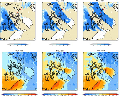
Fig. 7 Same as Fig. 6 but for 24-hour forecasts.

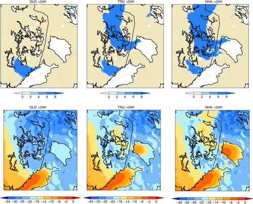
The low-level cloudiness affected the predicted screen-level temperature (Figs. 6 and 7, lower panels). OLD predicted uniformly cold temperatures, as could be expected in such meteorological situation under clear sky and over snow- or ice-covered surface. In TRU and NHA, the air temperature was higher both over Lake Ladoga and over the cloudy land areas northwest of the lake. Over the lake, the temperature followed the ice distribution, as could be expected.

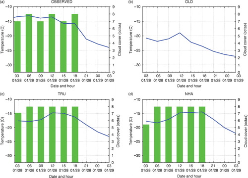
Relations between the predicted and observed temperature and low-level cloudiness were studied in detail by comparing the observations and forecasts at two weather stations, Ilomantsi Mekrijärvi (02939, marked as 1 in Fig. 5a, hereafter Ilomantsi) and Joensuu Linnunlahti (02928, marked as 2, hereafter Joensuu). The distance between the stations is only about 60 km. Note that these stations are different than those chosen for illustration of the temperature fluctuations during the whole anticyclonic period in Fig. 2. The cloud passed the weather stations at slightly different times, thus motivating us to compare this timing in different experiments. The closest predicted gridpoint values from the three forecasts were chosen for comparison.

The observed low-level cloud cover and temperature at Ilomantsi and Joensuu are shown in Figs. 8a and 9a as a function of time, respectively. As observed at Ilomantsi, the sky was covered by low clouds from 06 UTC to 15 UTC, while at Joensuu the sky was cloudy from 03 UTC up till 18 UTC. As a consequence, at Ilomantsi the temperature rose from −28°C to −18°C in 12 hours when the sky became cloud-covered. Because of the clouds, the temperature change was not, at least entirely, due to the normal daily cycle driven by the solar radiation. When the cloud disappeared after 15 UTC, the temperature dropped from −18°C below −30°C. At Joensuu, the temperature was around −15°C all day due to the cloudiness, i.e. in the early morning hours it was 15°C warmer than at the nearby Ilomantsi. During the cloudy phase, the cloud base height varied at Ilomantsi from 30 m to 120 m and at Joensuu from 70 m to 180 m. At Joensuu also fog was reported. Both stations reported light snowfall, but the amount was too small to be detected in the precipitation measurements.

Fig. 8 Observed and predicted 2-m air temperature (°C, blue line, left y-axis) and instantaneous low-level cloud cover (octas, green bar, right y-axis) at Ilomantsi (WMO station number 02939): Observed (a), predicted by OLD (b), predicted by TRU (c), and predicted by NHA (d).

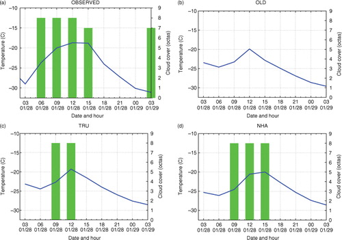
The corresponding forecasts (Figs. 8b–d and 9b–d) reveal the striking differences between the experiments: there was no low-level cloud in OLD, neither at Joensuu nor at Ilomantsi. Much more realistic cloud cover was predicted by both TRU and NHA. Looking more closely at the forecasts at Ilomantsi (Fig. 8), the duration of the cloudy period was underestimated by these experiments. When there were clouds, the cloud base heights (diagnosed from the existence of liquid or ice water within the model's vertical resolution) were predicted well by both TRU and NHA: while the observed values at 09, 12, and 15 UTC were 60, 90, and 120 m, the predicted values were 66, 66 m, and no cloud in TRU, and 66, 66, and 105 m in NHA. The heights of cloud tops varied between 240 and 290 m in TRU and between 270 and 360 m in NHA. To summarise, NHA predicted more clouds than TRU and they were thicker. This difference was also seen in the values of vertically integrated cloud condensate. This is the sum of specific liquid and ice content, in this case consisting mostly of liquid. In TRU the values varied between 9–13 gm⁻² and in NHA between 11–22 gm⁻² when the cloud was present. The vertical distribution of cloud condensate revealed that it was in both experiments concentrated in the lower atmosphere, indicating that only low-level clouds were predicted. For the cloud condensate and the height of low cloud tops we had no observations for verification.

At Joensuu (Fig. 9), the low-level cloud cover and the sky clearing were forecast correctly by TRU and NHA. However, both experiments predicted similarly the cloud base heights somewhat too low, giving values between 60 and 100 m, while observations indicated values between 70 and 180 m. The cloud tops were higher in NHA, between 270 and 360 m, than those in TRU, which predicted values between 200 and 290 m. Thus the clouds were thicker in NHA than in TRU, as was the case at Ilomantsi. The vertically integrated cloud condensate varied in TRU between 8–24 gm⁻² and in NHA between 12–37 gm⁻², which are all realistic values for shallow boundary layer clouds. As at Ilomantsi, the TRU and NHA cloud condensate was concentrated in the lower atmosphere indicating that only low-level clouds were predicted.

Fig. 9 As Fig. 8 but at Joensuu (WMO station number 02928).

The thicker cloud in NHA compared to TRU both at Ilomantsi and Joensuu was indicated also by the downward LWD. LWD values were constantly around 165 Wm⁻² in the clear-sky experiment OLD while the maximum values by TRU and NHA at Ilomantsi in the afternoon were 207 Wm⁻² and 222 Wm⁻², respectively. The corresponding values for Joensuu were 231 Wm⁻² and 263 Wm⁻².

The amplitude of screen-level temperature at Ilomantsi was forecast rather similarly too small by all experiments (Fig. 8). The maximum daytime temperatures were reasonable and the cooling in the evening was predicted correctly, although the night minimum temperature remained several degrees too high. At Joensuu, the temperature in OLD was too low by 5–10°C during the whole forecast due to the unpredicted clouds (Fig. 9). In TRU and NHA, the temperatures were quite well predicted, especially at noon and in the afternoon, thanks to the good low-level cloud forecast. However, in the morning of 28 January both experiments predicted too cold temperatures by 5°C, presumably due to inaccurate prediction of the cloud evolution during the first hours of the simulations. The cooling in the evening and at night in TRU and NHA was well predicted, although the observed minimum temperatures were again not reached.

The cold morning temperature on 29 January at Ilomantsi (Fig. 8) remained unpredicted, although no experiment showed clouds. Atlaskin and Vihma (2012) reported that all NWP models have problems in predicting cold enough temperatures in the stable boundary layer situations, where they show increasing bias with decreasing temperature and strengthening temperature inversion. In a review of the results from the Global Energy and Water Exchange (GEWEX) Atmospheric Boundary Layer Studies (GABLS), Holtslag et al. (2013) reported an obvious result from their studies that operational models typically have too much mixing in stable conditions, which strongly impacts diurnal cycle of temperature and other near-surface variables. They also stated that coupling between the atmosphere and the land surface is the key for a good representation of the diurnal cycle of the boundary layer variables. Next, in Section 4.3, we analyse in detail the surface energy balance and cloudiness in order to understand the differences between experiments.

In summary, our experiments showed that a precise forecast of the cloud cover was crucial to improve the temperature forecast. Only those experiments, which relied on realistic ice conditions over Lake Ladoga, were able to predict the clouds and their movement. This, in turn, improved the temperature forecasts. Provided with these forecast maps by HIRLAM, a forecaster would predict the variations of temperature in Eastern Finland.

4.3. Boundary layer and conditions over land and lake

So far we have discussed the influence of frozen or unfrozen Lake Ladoga on the near-surface temperature and cloudiness in Eastern Finland. In this section, we illustrate the simulated boundary layer structure and surface energy balance with examples at two locations: one at a point over the central part of Lake Ladoga and one over land at Ilomantsi. The 24-hour predicted temperature and dew-point (Fig. 10a) and wind speed (Fig. 10b) profiles are shown for point L over Lake Ladoga (see the map in Fig. 5) in the lowest 2-km layer. Above the atmospheric boundary layer, the results of three experiments – OLD over ice, NHA over open water and TRU over a freezing surface – were in agreement with each other. Above the inversion, the atmosphere was very dry, as characterised by the large dew-point deficit Δ=T−T _d ≈20°C. The maximum wind speed was reached at the top of the inversion layer. However, inside the boundary layer, the experiments showed remarkable differences in the profiles.

Fig. 10 Twenty-four-hour predicted temperature (solid line) and dew point (dotted line) (a) and wind speed (b) profiles at the gridpoint over Lake Ladoga marked with L in Fig. 5 from three experiments: OLD (red), TRU (green) and NHA (blue). The valid time of the profiles is 29 January 00 UTC.

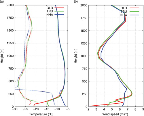
In experiment OLD (ice-covered lake surface), the surface-based temperature inversion was strong, about 15°C between the surface and the ca. 300-m level. The wind was very weak close to the surface, where the smallest Δ≈2.5°C was suggested by the model. These profiles over ice resembled those of the snow-covered land surface (not shown). This experiment assumed frozen Lake Ladoga, which excluded the source of moisture, available for the experiments TRU and NHA. We can assume that there was not enough humidity for formation of clouds in the shallow stable boundary layer of OLD, where mixing was also reduced. There may have been a small probability of local ice fog formation just above the ice.

NHA (open water) profiles represent conditions over an ice-free lake surface. Due to the large temperature difference between water and air, the turbulent fluxes were strong, causing strong mixing in the planetary boundary layer. The mixed layer was the thickest and warmest among the three experiments but still reached only the height of ca. 300 m, where it was capped by an elevated inversion. The near-surface turbulence lifted the inversion from surface to the top of the relatively shallow boundary layer. This is typical for anticyclonic conditions, where a large-scale descending motion is prevailing. The wind maximum at the top of the capping inversion showed only a minor difference from the mean wind speed in the boundary layer. The boundary layer temperature profile indicated neutral or slightly unstable conditions. Moisture evaporated from the lake was mixed to the whole boundary layer. However, the relatively weak wind shear reduced the simulated mixing somewhat. All this favoured cloud formation but not sufficiently to trigger deep convection and snowfall.

In experiment TRU, lake properties were handled by the prognostic parametrisation by FLake, which was coupled to the atmospheric model at every time step. Therefore, in any gridbox containing a fraction of lake, water temperature or ice depth evolved during the forecast. At the gridpoint L, Lake Ladoga became frozen during this forecast about 12 hours before the time of the predicted wind, temperature and humidity profiles shown in Fig. 10. As seen in Fig. 11, the surface (now ice) temperature started to decrease after freezing at noon, but there was not enough time for the surface-based temperature inversion to build to the strength shown by OLD. Hence, the profiles were between those predicted by NHA and OLD. However, evaporation from the lake and mixing started to decrease immediately after the freezing (Fig. 11). Some of the neighbouring gridboxes still remained ice-free, therefore influencing the profiles in gridpoint L. No cloud was predicted by TRU in this gridbox.

Fig. 11 Predicted surface fluxes (unit Wm⁻², left y-axis), averaged over 3 hours, and temperatures of ice and water (unit °C, right y-axis) during 28 January 2012 at the gridpoint over Lake Ladoga marked with L in Fig. 5 as given by the experiment TRU. No clouds were predicted by TRU at this location. All fluxes are denoted positive towards the surface, both from above and below.

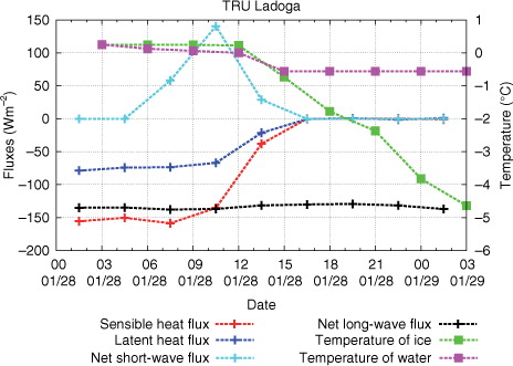
Figure 11 shows the evolution of the latent and sensible heat, net short-wave and LWD fluxes together with the predicted lake temperatures at the gridpoint L. The figure is based on one forecast from experiment TRU, initiated from 28 January 00 UTC analysis. Note that in HIRLAM convention all fluxes are denoted positive towards the surface, both from above and below. At the beginning of the forecast the lake was ice-free. LSWT by FLake was close to zero, indicating that water was close to freezing. Due to the cold air mass above, the latent and sensible heat fluxes were quite large and negative, −70 Wm⁻² and −150 Wm⁻², respectively, thus directed from the lake to the atmosphere. Turbulent mixing in the boundary layer was reduced by the prevailing stable conditions and moderate wind shear. However, the moisture flux was sufficient for the formation of the low cloud over Lake Ladoga. This cloud then propagated downstream and dramatically affected the screen-level temperatures far from the lake.

Energy balance over the water or ice surface is the sum of the turbulent heat fluxes, the net long-wave and short-wave radiation fluxes and the heat transfer from below. The transfer from below, estimated by FLake in the experiment TRU, was very small before and after freezing. During the day, when there was still no ice, the water surface heat balance was negative (fluxes directed from the lake to the atmosphere). This resulted in ice formation. When ice appeared, its surface heat balance was still negative, and the ice surface temperature started to drop very fast. Hence, the turbulent heat fluxes decreased and approached zero in the stable surface layer. During the night, the surface lost heat only due to the net LWD. The ice depth continued to increase, and the ice temperature continued to drop. At the end of the forecast, the ice temperature had decreased almost to −5°C. During the next day, the increased albedo of the now ice-covered lake surface would lead to less absorption of the solar radiation and further cooling of the surface.

At a point over land, the surface energy balance evolved differently under the clear sky and low clouds. The fluxes and surface temperatures at Ilomantsi from TRU (Fig. 12) are shown for the same period as the temperature and cloud cover in Fig. 8c. Of the Ilomantsi grid square, 41% was covered by frozen (small) lakes, while the rest was mainly snow-covered forest. On midday 28 January, the low clouds were forecast by HIRLAM. At that time the net short-wave flux towards the surface was only one third (ca. 50 Wm⁻²) of that at the clear-sky gridpoint over Lake Ladoga (Fig. 11). The net long-wave radiative flux was small and negative, ca. −20 Wm⁻² and thus directed from the surface to air. In this situation, the long-wave cooling was prevented by the low-level cloud cover. A small sensible heat flux (ca. −15 Wm⁻²) was negative and thus directed from the surface to air.

Fig. 12 As in Fig. 11 but for Ilomantsi and temperature of forest surface instead of LSWT. Cloudy time period is shown with shading. Ice temperature represents the local small lakes in the Ilomantsi gridbox. Note that the scale in the y-axis is different to Fig. 11.

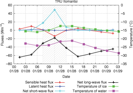
The surface temperature in the snow-covered forest reached a maximum value of ca. −22°C in the afternoon (Fig. 12). The ice surface temperature, predicted by FLake for the lake part of the gridbox, was much higher during the whole period, with a maximum value of ca. −13°C. In the evening, when the cloud disappeared, the net long-wave cooling increased and approached value of −60 Wm⁻². This was less than half of the corresponding value at the gridpoint over Lake Ladoga (Fig. 11). However, it was sufficient to cause a decrease of the forest snow and lake ice surface temperatures, since the long-wave flux was only compensated by the smaller heat flux from the snow-covered soil or lake ice. It is known that both in the model and in the nature, even a rather thin layer of snow is sufficient to insulate the relatively warm soil (or thin lake ice) from the air. As seen in Fig. 8a, cooling of the surface led to cooling of the near-surface air, which continued the whole night, as correctly suggested by experiment TRU.

In this section, we diagnosed the boundary layer and surface conditions of the HIRLAM forecasts. There were no flux observations for the validation of the simulated surface energy balance. However, according to the resulting temperature and cloud forecasts, the winter-time boundary layer over water and snow was described well by HIRLAM.

4.4. Objective verification

Strictly speaking, the influence of lakes on weather and climate is not local but is spread to the surroundings of the lake. Scott and Huff (1996) reviewed several earlier studies and concluded that the influence of the Great Lakes extends over a distance from 10 km to more than 100 km, depending on the weather parameter and also on the lake in question. The influence can be different on different sides of the lake. These authors used an 80-km wide zone when estimating the size of climatological lake-effect of several weather parameters.

In the current case, the maximum influence of Lake Ladoga can be estimated to extend as far as the lake-originated cloud was spread by the wind. In the upwind direction, the influence extent would be small. Based on Fig. 3, the cloud was detected at least 250 km to the west and northwest of the lake. The predicted wind direction over Lake Ladoga at the height of the low clouds in all experiments was from southeast, turning later more towards east and a low-level jet was predicted at the height of 250–300 m (not shown). Hence, the observing stations on the western side of Lake Ladoga up to 250 km were selected, 10 stations in total, for the objective verification. Exactly the same observations were included in the verification of different experiments. The validation time period was from 25 January to 5 February.

The bias and rms-error of 2-m temperature forecasts as a function of forecast length are shown in Fig. 13. The values at the initial time are analysis errors and are therefore not comparable to the forecast errors. Typically to the short-range 2-m temperature forecasts, there was no large growth in the bias or rms-error with the forecast length. The differences between experiments were large, but similar at all forecast lengths. Concerning the bias, OLD had the largest negative error, of the order −2°C or more. In NHA the bias was of the order −0.5°C and in TRU even less. Because the only difference between experiments was the state of Lake Ladoga, it is evident that the correct ice conditions of Lake Ladoga improved the temperature forecasts also when measured with objective scores and averaged over a longer time period.

Fig. 13 Bias and rms-error of 2-m temperature as a function of forecast length for the period from 25 January to 5 February and averaged over 10 observing stations westwards and closer than 250 km from Lake Ladoga. Forecasts from 00 UTC and 12 UTC analysis are included in the statistics.

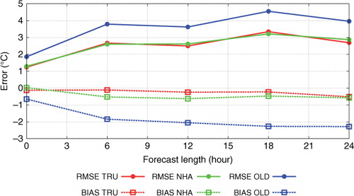
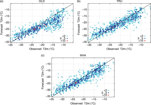
The large negative bias of OLD may look surprising, because normally in cold situations NWP models typically have difficulties to predict cold enough temperatures (Atlaskin and Vihma, 2012). The explanation is seen in Fig. 14, which shows the scatterplot of observed vs. predicted temperatures in different experiments. In all experiments, the extremely cold temperatures below −30°C were predicted too warm, as expected. The large negative bias in OLD was seen mainly in the observed temperature range −12°C to −18°C, which was typical for the cloudy conditions. In the observed cloudy conditions, OLD predicted too little cloud and hence too cold screen-level temperatures in this temperature range. Within the temperature range −20°C to −30°C (presumably clear-sky cases) the results were rather similar in all experiments. Far from Lake Ladoga the differences in verification scores of all parameters between experiments were very small (not shown).

Fig. 14 Scatterplot of observed temperature vs. predicted temperature for the same 10 stations as in Fig. 13 for OLD (a), TRU (b) and NHA (c). The time period is from 25 January to 5 February and +06-, +12-, +18- and +24-hour forecasts are included. Colours show the number of cases at each point as shown in the legend.

The time-series of observations and forecasts indicated that largest differences between forecasts took place during the last week of January, i.e. time when the ice conditions of Lake Ladoga were different in different experiments (not shown). The coldest period in Eastern Finland was observed during the first week of February. Lake Ladoga was then almost frozen in reality and completely frozen in all experiments. During this period, the temperature forecasts by different experiments were close to each other (not shown).

Summarising the results of objective verification, we conclude, that the correct description of the ice conditions over Lake Ladoga improved the temperature verification scores against measured temperatures in the vicinity of Lake Ladoga during the anticyclone period in January–February 2012. The verification also showed that the known inability of HIRLAM (and presumably also other NWP models) to predict very cold near-surface temperatures in the stable clear-sky cases still remains, independently of the surface description.

5. Summary

This study was inspired by a note in a local newspaper on 31 January 2012 about exceptional temperature fluctuations in Southeastern Finland. According to the note, the reason for the observed temperature fluctuations was a cloud spread from Lake Ladoga. For the duty forecaster, this situation was challenging, because a correct forecast of formation and movement of the cloud was necessary in order to predict the local temperatures. This case was also related to a series of studies, aimed at improving the treatment of lake effects in the HIRLAM NWP system.

Earlier, most of the studies on the effect of lakes on local weather have focused on severe convective snowfall cases. This case represents anticyclonic winter conditions, which typically means clear sky, stable stratification and cold near-surface temperatures. In such conditions, the individual processes may not be strong, but their subtle balance and interactions determine the weather, in this case the temperature variability. Thus, this case was a good test-bench for the physical parametrisations of HIRLAM, in particular for testing the sensitivity of the model to the description of the changing lake surface state.

We ran three experiments, which differed from each other only in the way the state of Lake Ladoga was described: based on climatology (experiment OLD), on a lake model (TRU) or on the analysis of satellite observations (NHA). Experiments based either on the assimilated satellite observations or on the prognostic lake parametrisation alone, indicated freezing of Lake Ladoga in the last days of January, which was in accordance with the observations.

When given the correct Lake Ladoga surface conditions, in one way or another (experiments TRU and NHA), the forecast model was able to predict the cloud formation and movement in a realistic way. Physically reasonable surface energy balance, predicted under clear and cloudy conditions, ensured a realistic prediction of the near-surface weather conditions. This made it possible for HIRLAM to forecast correctly also the 2-m temperature variations, which was confirmed by comparison with the observations. However, even small errors in timing of the cloud movement were found to make the temperature forecasts less accurate.

The period with strongly varying temperatures, due to the distribution of clouds, lasted only a few days. Objective verification scores were computed using the observations within a distance of about 250 km downstream (westwards) of Lake Ladoga over the whole anticyclonic period (2 weeks). They revealed a clear improvement of the 2-m temperatures, predicted by the experiments with a correct state of Lake Ladoga, as compared to the climatology-based experiment. The influence of Lake Ladoga was visible neither in the scores of the other surface-related parameters nor in the temperatures over a large area or over a long validation period.

In this study, we arrived at three main conclusions. First, the encouraging message was that HIRLAM could predict the effect of Lake Ladoga on local weather in this meteorological case, if the lake surface state was known. Second, the current parametrisation methods of atmospheric processes and air–surface interactions may lead to realistic description of the evolving anticyclonic boundary layer conditions, with the subtle balance between processes due to the large-scale atmospheric motion, local surface properties, radiation and turbulence. Third, these results encourage work towards a better description of the lake surface state in NWP models by fully utilising satellite observations, combined with advanced lake parametrisation and data assimilation methods.

6. Acknowledgements

The constructive comments of three anonymous reviewers significantly helped to improve the manuscript. We thank Janne Kotro for help in the interpretation of NOAA satellite images. This research was supported by European Space Agency (ESA-ESRIN) Contract No. 4000101296/10/I-LG (Support to Science Element, North Hydrology Project). Support by the International HIRLAM-B programme is acknowledged.

Notes

¹Forecasters’ practice is to estimate cloud formation probability from the dew-point deficit, shown by the sounding observations. A rule of thumb is that Δ smaller than 2 degrees in a reasonably thick layer indicates cloud formation.

References

- Andersson T. , Gustafsson N . Coast of departure and coast of arrival: two important concepts for the formation and structure of convective snowbands over seas and lakes. Mon. Wea. Rev. 1994; 122: 1036–1049.
- Andersson T. , Nilsson S . Topographically induced convective snowbands over the Baltic Sea and their precipitation distribution. Wea. Forecast. 1990; 5: 299–312.
- Atlaskin E. , Vihma T . Evaluation of NWP results for wintertime nocturnal boundary-layer temperatures over Europe and Finland. Quart. J. Roy. Meteor. Soc. 2012; 138: 1440–1451.
- Avissar R. , Pielke R. A . A parameterization of heterogeneous land surfaces for atmospheric numerical models and its impact on regional meteorology. Mon. Wea. Rev. 1989; 117: 2113–2136.
- Cordeira J. M. , Laird N. F . The influence of ice cover on two lake-effect snow events over lake Erie. Mon. Wea. Rev. 2008; 136: 2747–2763.
- Cuxart J. , Bougeault P. , Redelsberger J.-L . A turbulence scheme allowing for mesoscale and large-eddy simulations. Quart. J. Roy. Meteor. Soc. 2000; 126: 1–30.
- Daley R . Atmospheric Data Analysis. 1991; Cambridge University Press, New York, NY, USA. 457.
- Eerola K . Twenty-one years of verification from the HIRLAM NWP system. Wea. Forecast. 2013; 28: 270–285.
- Eerola K. , Rontu L. , Kourzeneva E. , Shcherbak E . A study on effects of lake temperature and ice cover in HIRLAM. Boreal Env. Res. 2010; 15: 130–142.
- Gollvik S. , Samuelsson P . A tiled land-surface scheme for HIRLAM. 2010. Unpublished manuscript. Online at: http://hirlam.org .
- Gustafsson N. , Nyberg L. , Omstedt A . Coupling of a high-resolution atmospheric model and an ocean model for the Baltic Sea. Mon. Wea. Rev. 1998; 126: 2822–2846.
- Holtslag A. A. M. , Svensson G. , Baas P. , Basu S. , Beare B. , co-authors . Stable atmospheric boundary layers and diurnal cycles: challenges for weather and climate models. Bull. Amer. Meteor. Soc. 2013; 94: 1691–1706.
- Kheyrollah Pour H. , Duguay C. R. , Solberg R. , Rudjord Ø . Impact of satellite-based lake surface observations on the initial state of HIRLAM – Part I: evaluation of MODIS/AATSR lake surface water temperature observations. Tellus A. 2014a; 66 21534, DOI: 10.3402/tellusa.v66.21534.
- Kheyrollah Pour H. , Rontu L. , Duguay C. R. , Eerola K. , Kourzeneva E . Impact of satellite-based lake surface observations on the initial state of HIRLAM. Part II: analysis of lake surface temperature and ice cover. Tellus A. 2014b; 66 21395, DOI: 10.3402/tellusa.v66.21395.
- Kourzeneva E. , Samuelsson P. , Ganbat G. , Mironov D . Implementation of lake model Flake into HIRLAM. HIRLAM Newsletter. 2008; 54–64. Online at: http://hirlam.org/ .
- Laird N. F. , Kristovich D. A. R. , Walsh J. E . Idealized model simulations examining the mesoscale structure of winter lake-effect circulations. Mon. Wea. Rev. 2003; 131: 206–221.
- Louis J. F . A parametric model of vertical eddy fluxes in the atmosphere. Bound. Lay. Met. 1979; 17: 187–202.
- Mironov D . Parameterization of Lakes in Numerical Weather Prediction. Description of a Lake Model. 2008; COSMO Technical Report 11, Deutscher Wetterdienst, Offenbach am Main, Germany.
- Mironov D. , Ritter B. , Schulz J.-P. , Buchhold M. , Lange M. , co-authors . Parameterisation of sea and lake ice in numerical weather prediction models of the German Weather Service. Tellus A. 2012; 64 17330, DOI: 10.3402/tellusa.v64i0.17330.
- Niziol T. A. , Snyder W. R. , Waldstreicher J. S . Winter weather forecasting throughout the Eastern United States. Part IV: lake effect snow. Wea. Forecast. 1995; 10: 61–77.
- Noilhan J. , Mahfouf J.-F . The ISBA land surface parameterisation scheme. Global Planet. Change. 1996; 13: 145–159.
- Noilhan J. , Planton S . A simple parameterization of land surface processes for meteorological models. Mon. Wea. Rev. 1989; 117: 536–549.
- Rontu L. , Eerola K. , Kourzeneva E. , Vehviläinen B . Data assimilation and parametrisation of lakes in HIRLAM. Tellus A. 2012; 64 17611, DOI: 10.3402/tellusa.v64i0.17611.
- Scott R. W. , Huff F. A . Impacts of the Great Lakes on regional climate conditions. J. Great Lake. Res. 1996; 22(4): 845–863.
- Sundqvist H . Inclusion of ice phase of hydro meteors in cloud parametrization for meso-scale and large scale models. Beitr. Phys. Atmosph. 1993; 66: 137–147.
- Sundqvist H. , Berge E. , Kristjansson J . Condensation and cloud parametrization studies with a mesoscale numerical weather prediction model. Mon. Wea. Rev. 1989; 117: 1641–1657.
- Undén P. , Rontu L. , Järvinen H. , Lynch P. , Calvo J. , co-authors . The HIRLAM-5 Scientific Documentation. 2002. Online at: http://hirlam.org .
- Vavrus S. , Notaro M. , Zarrin A . The role of ice cover in heavy lake-effect snowstorms over the Great Lakes Basin as simulated by RegCM4. Mon. Wea. Rev. 2013; 141: 148–165.
- Wright D. M. , Posselt D. J. , Steiner A. L . Sensitivity of lake-effect snowfall to lake ice cover and temperature in the Great Lakes region. Mon. Wea. Rev. 2013; 141: 670–689.