Loss of sea ice during winter north of Svalbard

Abstract

Sea ice loss in the Arctic Ocean has up to now been strongest during summer. In contrast, the sea ice concentration north of Svalbard has experienced a larger decline during winter since 1979. The trend in winter ice area loss is close to 10% per decade, and concurrent with a 0.3°C per decade warming of the Atlantic Water entering the Arctic Ocean in this region. Simultaneously, there has been a 2°C per decade warming of winter mean surface air temperature north of Svalbard, which is 20–45% higher than observations on the west coast. Generally, the ice edge north of Svalbard has retreated towards the northeast, along the Atlantic Water pathway. By making reasonable assumptions about the Atlantic Water volume and associated heat transport, we show that the extra oceanic heat brought into the region is likely to have caused the sea ice loss. The reduced sea ice cover leads to more oceanic heat transferred to the atmosphere, suggesting that part of the atmospheric warming is driven by larger open water area. In contrast to significant trends in sea ice concentration, Atlantic Water temperature and air temperature, there is no significant temporal trend in the local winds. Thus, winds have not caused the long-term warming or sea ice loss. However, the dominant winds transport sea ice from the Arctic Ocean into the region north of Svalbard, and the local wind has influence on the year-to-year variability of the ice concentration, which correlates with surface air temperatures, ocean temperatures, as well as the local wind.

• Sea ice
• Atlantic Water
• Svalbard
• heat transport
• air–ice–sea interactions

1. Introduction

Loss of Arctic sea ice remains one of the most visible signs of present and future global warming. The ice loss is now visible for all months and in all regions, but varies substantially between regions and time of year. Within the Arctic Ocean, the ice area decline has been largest during summer (Comiso, 2012). Despite a small recovery during summer 2013, the current September trend stands at −13.7% per decade (NSIDC).

To understand the different forcings that contribute to the loss of Arctic sea ice, it is important to study loss of sea ice in different regions, because several factors likely have contributed differently in each region. Sea ice responds to changes in heating or cooling reaching the surface layer, both from above and below. Heat is transported towards the Arctic with the atmosphere and the ocean, and in general, the Arctic air column is losing heat to space through outgoing longwave radiation.

Here we focus on the Whaler's Bay area north of Svalbard (black box in Fig. 1), the area where the warmest Atlantic Water (AW) inflow to the Arctic Ocean occurs. Aagaard et al. (1987), Saloranta and Haugan (2004), and Cokelet et al. (2008) estimated an ocean-to-air heat loss of 200–500 W/m² in this region, and stated that mixing between AW and colder ambient waters has provided sufficient oceanic heat to keep Whaler's Bay ice-free. Whaler's Bay is a prominent year-round polynya, and the AW heat may both prevent ice freezing during winter and melt the ice cover from below. Intense heat loss from the open ocean north of Svalbard modifies some of the AW by transforming it into Arctic intermediate water (Aagaard et al., 1987). How far into the Arctic Ocean the AW loses heat to the air, and how efficient the vertical mixing in this area is, are presently under discussion.

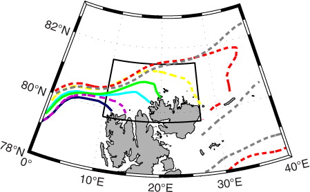
Fig. 1 Mean ice concentration field from 1979 to 2012, including the ice edge (15% ice concentration, solid black) and the mean ice concentration in the study region (48%, dashed black). The black box shows the study region north of Svalbard. The position of the West Spitsbergen Current (WSC) temperature measurements at Sørkapp is indicated in yellow, while the red arrow indicates the pathway of the Svalbard Branch of the WSC. The bathymetry is drawn as thin grey lines.

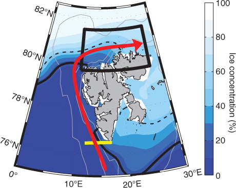
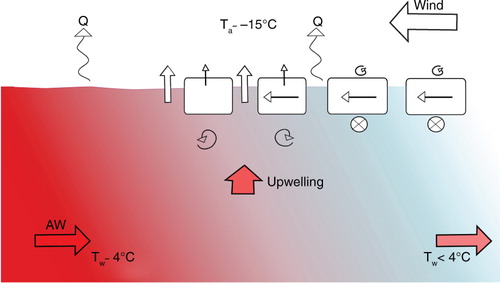
In this study we discuss the sea ice variability north of Svalbard and suggest possible drivers of the observed local ice area loss since 1979. The results indicate the AW warming as the main driver of the ice loss and as an important contributor to the atmospheric warming in the region. A sketch of the main processes occurring as the inflowing AW cools and meets the ice, driven in the opposite direction by winds, is shown in Fig. 2. In general, the winds bring along atmospheric air masses, so a wind from the north transports colder air towards Svalbard. Northerly winds also advect more ice from the transpolar drift stream into the region north of Svalbard. Presence of sea ice isolates the colder air, and contributes to colder air temperatures. Further, the wind could drive upwelling of AW along the Svalbard coast (Lind and Ingvaldsen, 2012). However, enhanced ice melt due to warmer AW creates a more stable freshwater layer underneath the ice, reducing further ice melt. According to Untersteiner (1988), the AW heat loss is sufficient to melt the advancing ice, maintaining the mean annual ice boundary at about 80°N.

Fig. 2 Schematic of air-ice-sea interactions north of Svalbard. Northerly winds transport sea ice from the Arctic Ocean (slightly deflected to the right) and bring cold air masses, facilitating larger ice cover. Upwelling of warm Atlantic Water (AW, reddish) melts the approaching sea ice, and a fresh, cold layer forms below the ice (bluish). Depending on the vertical mixing below the ice, the freshwater layer reduces further ice melt. The large ocean-to-atmosphere heat flux, Q, is strongly reduced by the presence of sea ice. In winter, Q is the sum of net longwave radiation, latent heat and sensible heat. Excess heat is lost to space through longwave radiation. T_a: air temperature, and T_w: water temperature.

2. Data and methods

In this work, we focus on the AW inflow region, so the datasets are bounded to the south by 79.7°N, to the north by 81.5°N, and lie within the zonal band 10–27°E (~60 000 km²)(Fig. 1). The datasets cover the years 1979–2012. Winter [December–March (DJFM)] and summer [June–September (JJAS)] means are calculated to describe the variability. Trends are estimated using linear least-squares regression, while two-sided t-tests are used to find significant levels for trends and correlations. Long-term trends in the datasets can increase the correlation coefficients, and moreover reduce the degrees of freedom. Quenouille (1952) defined the effective number of observations as:1

where n is the sample size, r ₁ and are the lag-1 autocorrelations of the two time series, r ₂ and are the lag-2 autocorrelations, and so on. To account for trends, we use the effective number of observations when estimating significant levels.

2.1. Sea ice

Daily averaged sea ice concentrations (percentage of ocean area covered by sea ice) are derived from passive microwave remote sensing data, using the NASA Team algorithm, from the Nimbus-7 Scanning Multichannel Microwave Radiometer (SMMR) and the Defense Meteorological Satellite Program (DMSP) Special Sensor Microwave/Imager (SSM/I), provided by the National Snow and Ice Data Center (NSIDC). Cavalieri et al. (1996) and references therein described the methods used to generate a consistent dataset from brightness temperature from the sensors. The dataset, with a resolution of 25 km×25 km, is spatially averaged over the study region north of Svalbard.

2.2. Atmospheric data

Daily atmospheric data are obtained from ERA-Interim reanalysis produced by the European Centre for Medium-Range Weather Forecasts (ECMWF). See Dee et al. (2011) and references therein for a detailed description of the reanalysis. Data of air temperature at 2 m height and wind at 10 m height are obtained at 12:00 UTC. The datasets have a spatial resolution of 0.75°×0.75° and are spatially averaged over the region north of Svalbard. Moreover, surface latent heat flux, surface sensible heat flux and surface net thermal radiation in the study region north of Svalbard and in an area west of Svalbard (5–15°E, 76–80°N) are reviewed.

2.3. AW temperature

AW temperature of the West Spitsbergen Current (WSC) westward from Sørkapp (Fig. 1) has been measured annually since 1977 by the Norwegian Institute of Marine Research. The results are based on data from the upper 50–200 m of a hydrographic section observed in autumn season (August–October). See Lind and Ingvaldsen (2012) for a more detailed description of the dataset. Missing data in 2003 and 2011 are linearly interpolated.

The AW temperature observations at Sørkapp are about 500 km upstream of our study region north of Svalbard (Fig. 1). Hence, the temperature observations are independent of the sea ice cover, wind and air temperature variability north of Svalbard. With a mean speed of 10 cm s⁻¹, the water at Sørkapp needs near two months to reach the study region, delaying the influence from the AW. Saloranta and Haugan (2001) showed coherent variations at 100–300 m depth near 76°N and 80°N during the 1980s and 1990s. For the analyses, AW temperature at Sørkapp in autumn is related to ice concentration north of Svalbard the following winter (i.e. AW temperature in autumn 1999 is compared to the ice concentration mean from December 1999 through March 2000). Hence ice concentration, wind and air temperature are lagging AW temperature by a few months for all analyses.

3. Results

The study region north of Svalbard (black box in Fig. 1) has an annual mean ice concentration of 48% between 1979 and 2012. Ice is present in all months with minimum ice concentration in September (Fig. 3). Largest ice cover is generally reached in April. The mean ice concentration field around Svalbard indicates the ice edge (15% ice concentration) near 80°N west of Svalbard (Fig. 1).

Fig. 3 Upper: Monthly averaged satellite-observed sea ice concentration (red line, September to September) including the standard deviation (grey region). The dashed line shows the annual mean ice concentration. Lower: The total 1979–2012 ice concentration reduction for each month is shown as black dots, with error bars indicating the 95% confidence intervals.

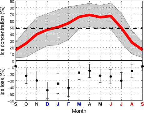
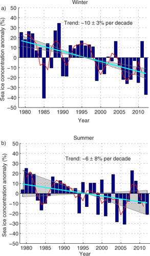
During the last three decades, the sea ice concentration has decreased north of Svalbard (Fig. 4), with record low annual minimum in 2012 (not shown). All months experience an ice loss, with largest negative trends in December, February and January, respectively (Fig. 3). The resulting winter (DJFM) ice loss is 10% per decade. August and September demonstrate the smallest reductions. The summer ice cover (JJAS) experiences an ice loss of 6% per decade and increased interannual variability since 1995 (Fig. 4b).

Fig. 4 Satellite-derived sea ice concentration anomalies north of Svalbard, 1979–2012. Dark blue is winter (a) and summer (b) means; and red shows the 3 yr running mean. The zero line represents the winter (56%) and summer (40%) 1979–2012 average. Linear trends are shown in light blue, and the shaded areas indicate the 95% confidence interval for the trend estimates.

The spatial winter ice loss north of Svalbard since the 1980s illustrates an ice retreat above the pathway of the AW (Fig. 5). Lower ice concentrations are gradually moving northeastward along Svalbard's northern coast. In 2012, the winter averaged 40% ice concentration contour line reaches almost 82 °N east of our study region, reflecting the second lowest winter ice minimum. Also the winter ice edge (15% ice concentration) has gradually shifted northeastward, retreating about 5° eastward and 0.5° northward since 1979 (not shown).

Fig. 5 Contour lines of the 40% winter (DJFM) ice concentration north of Svalbard during the 1980s (dark blue), 1990s (light blue), and 2000s (green). The most recent winters are also included with dashed lines (2010: yellow, 2011: purple, and 2012: red). In addition, February 2012 is shown in grey (dashed) to indicate a period with especially low ice concentrations, and ice-free areas extending towards Franz Josef Land. The black box indicates the study region.

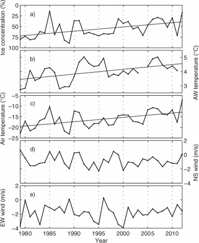
Time series of winter mean ice concentration, AW temperature, air temperature, north–south wind and east–west wind from 1979 to 2012 are shown in Fig. 6. Concurrent with reduced ice concentrations, Fig. 6b indicates an overall AW warming of 1.1°C since 1979. Moreover, the winter mean air temperature is rising by 6.9°C during the last 34 yr (Fig. 6c). These trends are significant on the 95% level. The air temperature shows large interannual variability concurrent with the variations in ice concentration. Easterly–northeasterly winds dominate north of Svalbard, however, with strong year-to-year variations (Fig. 6d and e). Slightly stronger northerly winds have apparently been simulated since 1979; however, the trends in winds are too small to be significant.

Fig. 6 Winter (DJFM) averaged sea ice concentration (a), AW temperature (b), air temperature (c), north–south wind component (positive from the south) (d), and east–west wind component (positive from the west) (e), 1979–2012. Note that the ice concentration (a) is inverted. Statistical significant linear trends (95%) are indicated by straight lines.

In order to find the main drivers of the winter sea ice variability, multivariate regression analyses were performed by analysing detrended and standardised AW temperature and north–south wind. Air temperature was not used due to the strong coupling between air temperature and ice concentration. Higher air temperatures cause less ice freezing, while presence of ice cover has a strong impact on air temperatures. Hence, we cannot differentiate between the predictor and the responder. The ice concentration regression based on AW temperature and north–south wind explains 32% of the variability in the satellite-derived ice concentration, suggesting that winter ice concentration variability on annual time scales is partly driven by variations in AW temperature and north–south wind. The east–west wind component was also tested, but did not increase the overall fit. EOF analyses of detrended and standardised values indicate that 58% of the combined variability (EOF1) is associated with high AW temperatures, high air temperatures, wind from the south and low ice concentrations (not shown).

4. Discussion

Concurrent with reduced ice concentrations in the area north of Svalbard, the AW and atmosphere have warmed over the last three decades. Despite the large air temperature rise of 6.9°C (Fig. 6c), the air temperature remains well below freezing during winter. Thus, higher air temperatures will have caused reduced ice freezing rather than enhanced ice melt. With wind-driven ice transport from the Arctic Ocean and strong direct interactions between AW and sea ice north of Svalbard, the early winter sea ice concentration can be described in terms of ocean temperature and north–south wind (r=0.56). Combinations of warm AW, high air temperatures and wind from the south are associated with reduced ice concentration north of Svalbard. The opposite is also true, cold AW and air temperatures, and stronger winds from the north, tend to increase the ice concentration. Onwards we discuss the influence of AW temperature, air temperature and wind on the reduced ice cover north of Svalbard, with the aim to explain the changes that have occurred.

Detrended winter ice concentration correlates significantly with north–south wind and air temperature (Table 1), suggesting large atmospheric influence on interannual variations in ice concentration. Northerly winds increase the ice concentration directly by transporting ice from the Arctic Ocean towards Svalbard, and indirectly by bringing colder air masses, enhancing ice freezing. Table 1 also shows significant correlation between detrended north–south wind and air temperature (r=0.51), suggesting that atmospheric circulation affects variations in winter air temperature on an interannual basis.

Table 1. Correlations between winter (DJFM) means

Ice	v	AW	Ta	u
Ice	—	− 0.50	− 0.20	− 0.90	0.11
v	−0.37	—	− 0.13	0.51	0.06
AW	−0.41	−0.17	—	0.27	− 0.05
Ta	−0.92	0.36	0.47	—	0.03
u	0.09	0.05	−0.03	0.04	—

The upper right triangle (roman) represents correlations between detrended time series, while the lower left triangle (italic) shows correlations including trends. Significant correlations within a 95% confidence level are marked with boldface. Ice: ice concentration, v: north–south wind, AW: Atlantic Water temperature, T_a: air temperature, u: east–west wind.

When it comes to the atmospheric trends, there is no statistically significant trend in the winds. Thus the significant negative trend in ice concentration since 1979 cannot be driven by the winds. The strong air temperature rise of 6.9°C over the 34-yr study period corresponds to a linear temperature trend of 2°C per decade. This trend is 20–45% larger than the trends observed for almost the same time span (1975–2011) at comparable sites further south [Ny-Ålesund 1.36°C per decade, and Svalbard Airport 1.66°C per decade (Førland et al., 2011)]. Because surface air temperature is closely coupled to the ice cover, we proceed to the other possible driver of the changes in ice concentration, the AW.

Increased heat transport by the WSC to our region increases the reservoir of heat below the sea ice, and given that vertical mixing is not a limiting factor, the ice cover experiences enhanced bottom melt and reduced ice formation. Increased AW heat transport in recent years with both warmer water and stronger flow, was discussed by Beszczynska-Möller et al. (2012), Piechura and Walczowski (2009) and Polyakov et al. (2012a). Model studies of the AW heat transport and bottom melting in the Arctic Ocean suggest that periods of increased heat transport lead to enhanced bottom melting (Alexeev et al., 2013; Sandø et al., 2014). Here, we only consider AW temperature, because there is no available current meter record before the 1990s.

AW temperature and ice concentration correlate with r=−0.20 when the trends are removed. However, if the trends are maintained, the correlation increases to r=−0.41 (Table 1). This may imply slow oscillations in AW temperature that last longer than the 34-yr long time series, or just a general linear warming. Such long-term oscillations in AW transport are documented in the Barents Sea where time series longer than 100 yr are available (Smedsrud et al., 2013). How much of an impact could a ~1°C ocean warming have on the sea ice cover and the atmosphere above? To answer that question we estimate some related heat budgets, and find that although AW temperature may not have a strong impact on interannual variations in ice concentration, the AW warming could drive the ice loss as well as the atmospheric warming in our region.

The heat capacity of the ocean is much larger than that of the air. To compare the two observed temperature trends, we first calculate the change in heat content of a column of water or air:2

where ΔQ is a change in heat content (J m⁻²), c is heat capacity (J kg⁻¹ K⁻¹), m is mass (kg m⁻²) and ΔT is a change in temperature. Assuming an atmospheric boundary layer height of 800 m, the atmospheric warming of 6.9°C increases the atmospheric heat content by 7.7×10⁶ J m⁻². A similar increase in heat content in the ocean can be achieved by an AW warming of 0.03°C in the upper 50 m of the ocean. Hence, an ocean warming of 1°C contains several orders of magnitude more heat (J m⁻²) than the observed atmospheric warming.

Assuming a steady AW transport of 3 Sv (Sv≡1×10⁶ m³ s⁻¹) (Beszczynska-Möller et al., 2012), the inflowing and exiting temperatures of the AW determine the heat transport. The time series in Fig. 6b shows the observed changes in inflow temperature, and we first use a representative AW temperature for around 1980 of 3.0°C. The AW temperature decreases along the WSC, and at 800 km downflow, at the eastern end of our area, the temperature has decreased to about 1.5°C (Cokelet et al., 2008). Based on the heat conservation equation at stationary conditions,3

where Q is the heat (W), ρ is the density of seawater (kg m⁻³) and V is the volume transport (Sv), the estimated current in 1980 would result in a heat transport of 36 TW at Sørkapp. Assuming an outflow temperature of 1.5°C (following Cokelet et al. [2008]), 50% of the heat would continue further into the Arctic Ocean. Unknown portions would go directly to the air before the AW reaches the ice-covered areas, to lateral mixing, and to melting of sea ice in our area. The winter mean ice concentration at the time was 75% (Fig. 6) and the atmospheric temperature was −20°C, implying a mean surface outgoing longwave radiation flux of 232 W m⁻² during winter.

In contrast to the situation in 1980, we know that the AW inflow temperature has increased with 1.0°C up to 2010, and that the ice concentration dropped to about 40%. A 1°C warming at Sørkapp implies an enhanced northward heat transport of 12 TW, assuming a constant AW flow. Unfortunately, there are no long-term observations of changes in outflow AW temperature. However, by comparing 1990–1995 observations with Russian climatologies, Grotefendt et al. (1998) described a ~0.5°C warming of the AW temperature at 500 m depth east of our area. Therefore, we assume that half of the extra heat due to the AW warming at Sørkapp carries on with the AW flow inside the Arctic Ocean, while 25% (3 TW) is available for melting sea ice, and the last 25% warm the air directly. This is consistent with assuming a change in outflow temperature from 1.5°C in 1980, to 2.0°C in 2010. During winter, a mean surface outgoing longwave radiation flux from the −13°C surface would be 259 W m⁻², that is, 27 W m⁻² larger than in 1980. This compares to 1.6 TW over our area (~60 000 km²), stating that a substantial part of the overall available extra heat, but not all, has reached the atmospheric boundary layer.

A rough estimate of atmospheric heat fluxes supports our assumptions concerning the heat budgets. ERA-Interim reanalysis indicates a slight increase in surface sensible heat flux, surface latent heat flux and surface net longwave radiation (outgoing fluxes) in the area north of Svalbard between 1979 and 2012 (not shown). Increased upward heat fluxes are also found above the WSC west of Spitsbergen (5–15°E, 76–80°N) (not shown). The reanalysis shows an increased upward heat flux of about 2 TW over the 1979–2012 period between Sørkapp and the outflow of our study region. This indicates that some heat is lost to the atmosphere, while most of the extra heat likely has contributed to melting of sea ice and warming of ambient waters.

Most of the ice reduction in the area around Svalbard has occurred in the study region north of Svalbard (Fig. 5). In our region, the ice cover has been reduced by 15 000 km² since 1979. An estimate of the heat needed to melt H meters of sea ice can be calculated using:4

where Q is the energy needed (J m⁻²), ρ _i is ice density (kg m⁻³) and L is latent heat of fusion (J kg⁻¹). Assuming that the extra available AW heat of 3 TW reaches the ice and is equally distributed over the study region, 2 m thick ice would melt in about four and a half months. However, with a winter mean ice concentration of 56%, ice-free waters may be reached faster.

The estimated available AW heat is thus clearly enough to cause the observed sea ice loss north of Svalbard, and the main winter ice loss above the core of the AW north of Svalbard suggests that the warm AW has reached the sea ice. Although increasing ice melt creates a more stable freshwater layer between the salty AW (S ~35) and the fresh sea ice melt, local wind mixing can provide energy for transfer of heat from the AW to the upper layer and consequently to ice melt and to the atmosphere (Rudels, 2012). The monthly mean sea ice advection speed during winter in our area is 2–6 cm/s (ftp://sidads.colorado.edu/pub/DATASETS/nsidc0116icemotionvectorsv2/browse/north/months/), suggesting a transit time of about 1–4 months. This means that the thickness of the entering sea ice is important, and may suggest that residence time above the AW is a more limiting factor than the available heat.

As the AW temperature is measured at Sørkapp, ~500 km upstream, it is independent of the air temperature rise and ice concentration loss north of Svalbard. An ocean-driven ice loss north of Svalbard would, however, result in stronger ocean-to-atmosphere heat fluxes locally. This is consistent with Polyakov et al. (2012b) who stated that local atmospheric warming over areas of ice loss is a response to, rather than a driver of, the declining ice cover. Our results indicate that part of the air temperature increase has been caused locally by the ice loss. Assuming an ocean-to-atmosphere open water mean winter heat flux of 200 W m⁻² (Smedsrud et al., 2013), the increased heat flux to the atmosphere caused by the extra 15 000 km² of open water (ice loss), would give an extra heating of 3 TW. This suggests that ~50% of the heat lost to the atmospheric boundary layer is lost through longwave radiation as calculated above (1.6 TW), and that the other half has been transported out of the region by atmospheric circulation. The ice loss above the AW pathway is therefore likely a driver of the atmospheric warming, and not vice versa. Climate projections indicate a substantial air temperature warming northeast of Svalbard due to reduced sea ice coverage (Førland et al., 2009).

Another indication of warm water as a major contributor to the ice loss is the large winter ice reduction, in contrast to the Arctic Ocean summer ice loss. With winter air temperatures well below freezing, the AW is the only heat source in the area north of Svalbard (Rudels, 2010), and largest AW influence is expected during winter. During summer other factors probably contribute more to the observed ice loss.

Warmer surface waters cause delayed ice formation and consequently lower ice concentrations in early winter. Our results agree with findings by Årthun et al. (2012) who compared observations and simulations for reductions in the Barents Sea winter ice cover due to increased AW heat transport. According to Årthun et al. (2012), an increase in AW heat transport to the Barents Sea of 10 TW has resulted in an ice reduction of 70 000 km². Based on these values the estimated extra oceanic heat transport to our area (3 TW) would potentially cause an ice reduction of 21 000 km². This is 40% larger than the observed loss in our area. The ice would be thicker in our area, and more ice would be formed elsewhere and transported in, so this could explain the different response. Ivanov et al. (2012) described a winter ice loss in the Western Nansen Basin, and observed a thinner and less extensive ice cover above the pathway of the AW there. They thus suggested an influence from the warmer AW on the winter ice reduction in that region, consistent with our results.

As the Arctic and the rest of the globe continue to warm, and the ice cover continues to decrease, a number of key elements remain almost unobserved. We have documented the warming in both the atmosphere and the ocean, and the decline in ice concentration since 1979, but we are lacking comparable time series for changes in AW volume transport, sea ice thickness and vertical mixing. Clearly the sea ice is probably thinner north of Svalbard now than in the 1980s, but the longest observational record of ice thickness started first in 1990 (Hansen et al., 2013), and covers the western side of Fram Strait. A response in sea ice concentration will only occur when the sea ice has thinned considerably, and might explain parts of the ‘missing response’ to the initial rise in AW temperature around 1990 (Fig. 6b).

Proper observations of ocean volume transport started in 1997 (Schauer and Beszczynska-Möller, 2009). Variations in volume transport before this time, and also how the total transport is distributed within the Arctic Ocean, remain unknown. The peak in total heat transport in 2004 seems to lead that of the temperature maximum occurring in 2006 (Schauer and Beszczynska-Möller, 2009). For ocean mixing in the Arctic, only snapshots in temporal and spatial coverage are available (Rainville and Winsor, 2008; Sirevaag and Fer, 2009). Any long-term changes, as well as a reasonable climatic annual mean for the region north of Svalbard, are not available.

The long-term prospects for Arctic sea ice are bad, especially for the summer ice. The large loss of the winter ice north of Svalbard is not typical for other regions inside the Arctic Ocean, but more in line with the ongoing changes in the Barents Sea over the last decades (Årthun et al., 2012). Now that the AW heat transport seems to have reached an all-time high value in 2004, a recovery of the winter ice could actually be expected over the next 10 yr. On the other hand, the sea ice is thinner, and vertical mixing could increase due to the reduced ice cover. It thus appears more difficult than ever to come up with future predictions.

5. Summary

Satellite observations north of Svalbard demonstrate reduced ice concentrations between 1979 and 2012. In contrast to other areas of the Arctic Ocean, the largest ice loss has occurred during winter with ~10% loss per decade. The summer ice loss trend is about half of the winter trend. Over the same period, the AW temperature has increased ~1°C and the regional winter air temperature has increased ~7°C, but there is no significant trend in the local wind.

Year-to-year ice variability is substantial, with winter means ranging between 15% and 90%. Although the winds apparently do not have impact on the trends, they have significant impact on the year-to-year variability. Low anomalies in sea ice concentration are consistently associated with winds from the south (less wind from the north), warmer air and higher AW temperatures.

The shrinking winter ice cover above the core of the AW indicates a direct influence from the AW on the ice conditions. Analytical estimates assuming constant volume flow and that ~25% of the heat transport reaches the ice-covered surface, indicate that the warmer AW has been a major driver of the ice reduction. Temporal changes in the vertical mixing of AW heat towards the ice, and long-term changes in sea ice thickness remain unknown, but may have played a significant role in the observed changes.

The decadal air temperature trend in our region is 20–45% higher than further south. This indicates that the local warming is forced by the increased oceanic heat transport, which has caused more open water and larger ocean-to-atmosphere heat fluxes. Because winter mean atmospheric temperature is still ~−10°C, the atmospheric warming would not lead to ice melting, but to reduced local ice growth.

6. Acknowledgements

This work was funded by the Centre for Climate Dynamics at the Bjerknes Centre through the Fast-Track Initiative grant. We thank Igor Polyakov and Asgeir Sorteberg for constructive and helpful comments that improved our manuscript.

References

- Aagaard K. , Foldvik A. , Hillman S. R . The West Spitsbergen Current: disposition and water mass transformation. J. Geophys. Res. 1987; 92: 3778–3784.
- Alexeev V. A. , Ivanov V. V. , Kwok R. , Smedsrud L. H . North Atlantic warming and declining volume of Arctic sea ice. The Cryosphere Discuss. 2013; 7: 245–265.
- Årthun M. , Eldevik T. , Smedsrud L. H. , Skagseth Ø. , Ingvaldsen R. B . Quantifying the influence of Atlantic heat on Barents Sea ice variability and retreat. J. Climate. 2012; 25: 4736–4743.
- Beszczynska-Möller A. , Fahrbach E. , Schauer U. , Hansen E . Variability in Atlantic water temperature and transport at the entrance to the Arctic Ocean, 1997–2010. ICES J. Mar. Sci. 2012; 69: 852–863.
- Cavalieri D. , Parkinson C. , Gloersen P. , Zwally H. J . Sea Ice Concentrations from Nimbus-7 SMMR and DMSP SSM/I Passive Microwave Data. 1996; Digital media, Boulder, Colorado USA: National Snow and Ice Data Center. Online at: http://nsidc.org/data/nsidc-0051.html .
- Cokelet E. , Tervalon N. , Bellingham J . Hydrography of the West Spitsbergen Current, Svalbard Branch: Autumn 2001. J. Geophys. Res. 2008; 113: C01006.
- Comiso J. C . Large decadal decline of the Arctic multiyear ice cover. J. Climate. 2012; 25: 1176–1193.
- Dee D. P. , Uppala S. M. , Simmons A. J. , Berrisford P. , Poli P. , co-authors . The ERA-Interim reanalysis: configuration and performance of the data assimilation system. Q.J.R. Meteorol. Soc. 2011; 137: 553–597.
- Førland E. J. , Benestad R. E. , Flatøy F. , Hanssen-Bauer I. , Haugen J. E. , co-authors . Climate development in North Norway and the Svalbard region during 1900–2100. 2009; Norwegian Polar Institute, Tromsø: Technical Report .
- Førland E. J. , Benestad R. , Hanssen-Bauer I. , Haugen J. E. , Skaugen T. E . Temperature and precipitation development at Svalbard 1900–2100. Adv. Meteorol. 2011; 2011: 14.
- Grotefendt K. , Logemann K. , Quadfasel D. , Ronski S . Is the Arctic Ocean warming?. J. Geophys. Res. 1998; 103: 27679–27687.
- Hansen E. , Gerland S. , Granskog M. A. , Pavlova O. , Renner A. H. H. , co-authors . Thinning of Arctic sea ice observed in Fram Strait: 1990–2011. J. Geophys. Res. 2013; 118: 5202–5221.
- Ivanov V. V. , Alexeev V. A. , Repina I. , Koldunov N. V. , Smirnov A . Tracing Atlantic Water signature in the Arctic sea ice cover east of Svalbard. Adv. Meteorol. 2012; 2012: 11.
- Lind S. , Ingvaldsen R. B . Variability and impacts of Atlantic water entering the Barents Sea from the north. Deep Sea Res. Part I. 2012; 62: 70–88.
- NSIDC. A better year for the cryosphere. Beitler, J. 2013, October. Online at: http://nsidc.org/arcticseaicenews/2013/10/a-better-year-for-the-cryosphere/ .
- Piechura J. , Walczowski W . Warming of the West Spitsbergen Current and sea ice north of Svalbard. Oceanologia. 2009; 51: 147–164.
- Polyakov I. V. , Pnyushkov A. V. , Timokhov L. A . Warming of the Intermediate Atlantic Water of the Arctic Ocean in the 2000s. J. Climate. 2012a; 25: 8362–8370.
- Polyakov I. V. , Walsh J. E. , Kwok R . Recent changes of Arctic multiyear sea ice coverage and the likely causes. Bull. Amer. Meteor. Soc. 2012b; 93: 145–151.
- Quenouille M. H . Associated Measurements.
- Rainville L. , Winsor P . Mixing across the Arctic Ocean: microstructure observations during the Beringia 2005 expedition. Geophys. Res. 2008; 35: 2L08606.
- Rudels B . Constraints on exchanges in the Arctic Mediterranean – do they exist and can they be of use? . Tellus A. 2010; 62: 109–122.
- Rudels B . Arctic Ocean circulation and variability – advection and external forcing encounter constraints and local processes. Ocean Sci. 2012; 8: 261–286.
- Saloranta T. M. , Haugan P. M . Interannual variability in the hydrography of Atlantic water northwest of Svalbard. J. Geophys. Res. 2001; 106: 13931–13943.
- Saloranta T. M. , Haugan P. M . Northward cooling and freshening of the warm core of the West Spitsbergen Current. Polar Res. 2004; 23: 79–88.
- Sandø A. B. , Gao Y. , Langehaug H. R . Poleward ocean heat transports, sea ice processes, and Arctic sea ice variability in NorESM1-M simulations. J. Geophys. Res. 2014; 119: 2095–2108.
- Schauer U. , Beszczynska-Möller A . Problems with estimation and interpretation of oceanic heat transport – conceptual remarks for the case of Fram Strait in the Arctic Ocean. Ocean Sci. 2009; 5: 487–494.
- Sirevaag A. , Fer I . Early spring oceanic heat fluxes and mixing observed from drift stations north of Svalbard. J. Phys. Oceanogr. 2009; 39: 3049–3069.
- Smedsrud L. H. , Esau I. , Ingvaldsen R. B. , Eldevik T. , Haugan P. M. , co-authors . The role of the Barents Sea in the Arctic climate system. Rev. Geophys. 2013; 51: 415–449.
- Untersteiner N . On the ice and heat balance in Fram Strait. J. Geophys. Res. 1988; 93: 527–531.